and Real Estate
∗
Rodrigo Mendes Pereira
†
Contents: 1. Introduction; 2. A Model of Investment in Buildings and Machines; 3. Empirical Assess-ment; 4. Concluding Remarks; A. Appendix 1.
Keywords:Investment; uncertainty; GARCH; panel data. JEL Code:C23; E22.
O investimento é geralmente tratado como uma variável homogênea na literatura. As grandes diferenças na natureza dos insumos emprega-dos em projetos de investimento levam a idéias interessantes que não são capturadas pela abordagem tradicional. Nesse artigo eu decomponho o investimento em máquinas e imóveis e examino o impacto da incerteza econômica sobre cada um desses componentes. Utilizando métodos de estimação com dados em painel para a indústria brasileira, encontramos evidências de que a incerteza reduz ambos os tipos de investimento. En-tretanto, o efeito parece ser mais intenso com máquinas, o que poderia ser uma conseqüência de um custo de reversibilidade mais alto.
Investment is usually treated as an homogeneous variable in the literature. The wide differences in the nature of inputs used in investment projects may lead to interesting insights that are not captured in the conventional approach. In this paper I decompose investment in machinery and industrial real estate and examine the impact of economic uncertainty on each of these components. Using panel data estimation methods for the Brazilian industry, I found that uncertainty exerts a harmful effect on both types of investment. However, the effect is much more intense with machines, which possibly is a consequence of their high reversibility costs.
1. INTRODUCTION
One of the most prominent topics of the modern research in investment theory has been the sen-sitivity of investment to changes in the level of uncertainty. The early models focus on the fact that
∗I thank an anonymous referee, and seminar participants at the University of Brasília, the Catholic University of Brasília, and
the XXIX Meeting of the Brazilian Econometric Society (Recife, Brazil, Dec 2007) for helpful comments.
†Instituto de Pesquisa Econômica Aplicada. Sbs Q1, Ed. BNDES, 3o andar, sala 314, Brasília, DF, Brazil – 70076-900,
greater uncertainty increases the marginal profitability of capital and, as a consequence, raises invest-ment (see Abel (1983)). This assertion is based on the convexity of the profit function in prices, which means that the average profit tends to be higher with volatile than with fixed prices.
In the late eighties and nineties economists have recognized the importance of the irreversible na-ture of investment on the theoretical discussion (see, for example, Pindyck (1988)). In essence, the introduction of asymmetric adjustment cost hypothesis sharply shifts the results, pointing out a nega-tive relationship between investment and uncertainty. The idea is to associate investment opportuni-ties with the rationale of financial options. A firm that decides to carry on an irreversible investment project abdicates the option of waiting for new information and postponing the rise in capacity. The economic value of this option rises in a largely uncertain environment. In this case, the increased fear of being committed to a project that turns out to be unprofitable leads to a delay in the decision in order to keep the investment option alive. By that means, uncertainty can hinder investment. Further contributions to the debate are given by Caballero (1991), who demonstrates that the degree of market competitiveness, besides the asymmetry of capital adjustment costs, greatly influences the sign of the investment-uncertainty relationship.
More recently, there have been some attempts to put the traditional theory and options approach together. Abel et al. (1996) emphasize that, in addition to the reversibility costs, firms also face expand-ability costs, since the acquisition price of capital may be higher in the future (due to the fact that the expanded capacity may also become profitable to the other competing firms, increasing the demand and the price of capital inputs). If a firm faces large expandability costs, a rise in uncertainty should induce firms to invest. This insight clarifies that, under both q-theory and options pricing approaches, uncertainty has an ambiguous effect on investment. The balance between reversibility and expand-ability costs determines whether an increase in uncertainty yields a discouragement or an incentive to invest.
The ambiguity of analytical findings stimulated the emergence of an empirical literature mostly directed to the U.K. and U.S. cases.1 A number of studies deal with aggregate data using time series methods (see Price (1995, 1996)). There has been, however, a growing number of authors who use panel data techniques applied to groups of industrial companies (Henley, 1999), industrial sectors (Campa and Goldberg, 1993) and developing countries (Sérven, 1998, Pindyck and Solimano, 1993). These works conclude mostly that more uncertainty leads to less investment.
In this paper we consider the heterogeneity of production goods, in the sense that investment may have different properties whether it is in the form of machinery or in the form of real estate. The issue of investment heterogeneity has been tackled before in the literature. A recent example is the work of Cruz and Pommeret (2006), in which embodied technology is introduced in a Pindyck (1988) framework of investment under uncertainty. These authors introduce capital heterogeneity in the sense that every capital has a certain vintage. Capital vintages differ in terms of the amount of energy required for them to operate.
Here we introduce an idea that, to the best of our knowledge, has not yet been addressed in the literature, which is the fact that uncertainty may not affect different types of investment in the same way. For example, investment in industrial real estate is typically much less industry- and firm-specific than investment in machines. While the resale of used machinery may face thin markets with few potential buyers, there are numerous possibilities for the conversion of an industrial building, or even a white-collars office building, into other economic usage. Therefore, one should expect that buildings have smaller reversibility costs than machines. Intuitively, the implication would be that an increased uncertainty worsens investment in machinery much more than investment in buildings. In this paper the validity of this assertion is examined. To do so, I build a model a la Abel et al. (1996), in which reversibility and expandability costs play a key role. However, I split capital stock into buildings and machinery. The idea is to analyze how these two forms of investment react to changes in their resale
and future purchase prices. The model provides theoretical support for an empirical investigation of the relationships between uncertainty and both types of investment. Along these lines, I use panel data techniques in a sample of twenty-two Brazilian industrial sectors with thirty years of annual data.
The issue of how to measure uncertainty is also discussed in the paper. Most of the empirical studies of uncertainty and investment use sample variability as a proxy for uncertainty. However, this proxy lacks accuracy as long as rational agents may partly predict fluctuations using information contained in their past behavior. Uncertainty should correspond only to the unpredictable changes of the variable. We follow Sérven (1998), adopting an alternative measure of uncertainty, based on the estimation of a generalized conditional heteroskedastic (GARCH) model.
The paper is organized as follows. Section 2 presents the extended version of Abel’s model, with investment in Buildings and Machines. Section 3 sets out the empirical approach and presents the main results for the Brazilian economy. Final conclusions are presented in section 4.
2. A MODEL OF INVESTMENT IN BUILDINGS AND MACHINES
2.1. The Problem of the Firm
A firm that decides to hold an investment project typically acquires several types of capital goods. The rise in capacity may involve the construction of a new building, the acquisition of machines, or even the purchase of computers, trucks and other durable goods used in the production process. A given expansion of capital stock can be accomplished through different investment plans. A natural question that comes up from such assertions is to know whether the mechanisms that drive investment decision are the same for the different types of investment. Specifically, do the macroeconomic circumstances that stimulate the purchase of new machines also favor a building-intensive investment project?
A great part of the recent investment literature has combined the uncertainty over future profitabil-ity of capital with the fact that investment may be partly or completely irreversible. In this regard, an important result is that the effect of uncertainty on investment depends on its degree of irreversibility. The larger are the discounts involved with capital stock resale, the most attractive is the option of wait-ing for new information and postponwait-ing the investment decision in an uncertain environment. Thereby, when capital cannot be easily reverted, uncertainty tends to hamper investment more intensely.
Interesting insights can be attained through the disaggregation of capital stock into its two main components, namely, machines and buildings. An important stylized fact is that the former is much more firm- and industry-specific than the later. A shoe factory building that shelters the production line may be directed, for example, towards a furniture manufacturing process when the market conditions for shoes change adversely. Yet, the machines used to produce shoes cannot be easily sold due to narrow markets. Certainly there are not many potential buyers for such machines. Besides that, the few possible buyers are subject to the same adverse market conditions that lead to the firm’s decision of selling its capital stock. The shoe manufacturer is induced to sell the equipment exactly when no one else is interested in acquiring it.
We consider a representative firm that chooses, in period one, the amount of capital stock to be used in the manufacturing process, being aware that this choice cannot be easily modified in period two. The innovation is to split capital stock into buildings,B, and machines,M. First-period choices are given byB1andM1. With such levels of inputs the firm obtains a first-period return ofr(B1, M1)
, whererB >0, rM >0, rBB <0, rM M <0andrM B >0. Therefore, the return function is strictly
increasing and strictly concave in both arguments. The latest inequality implies that machines and buildings are complements in the sense of having a small elasticity of substitution, which seems to be a sensible assumption. First-period prices of buildings and machines are given byβandµ, respectively. In the second period the firm earns a return ofR(B, M, e), whereeis a stochastic shock with c.d.f. given byF(e). The return function has the same properties in both periods. The only difference is that in the second period the return becomes stochastic. We assume thatRe>0, RBe>0andRM e >0,
which means that a positive shock increases not only the level of returns, but also the marginal return of both inputs.
The next step is to define three critical values for the shock terme: a small positive shockeH, a small
negative shockeL, and a large negative shockeM L. The valueeHis such thatRB(B1, M1, eH) =βH
andRM(B1, M1, eH) =µH , whereβHandµHare the second-period purchasing prices of capital in
the form of buildings and machinery, respectively. We assume that the second-period purchasing prices of both types of capital are higher than their respective first-period current prices, that is,βH> βand
µH > µ. If capital stock is not altered,eH is the precise value of the shock that equates the
second-period marginal return of capital to its second-second-period purchasing price. For the sake of simplification, we assume that this value is the same for the two types of capital.
If the shock is positive but smaller thaneH, marginal returns will be lower than purchase prices and
the firm will not change its first-period capital stock. The expansion of capital stock will be profitable only when the stochastic shock is at least as large aseH. The valueeL is assumed to be the level of
shock that equates second period marginal return of building units with their resale price. It is defined byRB(B1, M1, eL) = βL , whereβL < βis the resale price of a building unit. The hypothesis of
a small reversibility cost of buildings implies that the resale price,βLis slightly lower than the
first-period purchasing price, β. By that means, the equality among marginal return and resale price of buildings is achieved with a relatively mild negative shock in the second period.
Investment in machinery, on the other hand, is assumed to be highly irreversible. This irreversibil-ity can be defined as a large difference between first-period acquisition and second-period resale prices. Therefore, the value of the negative shock that equates marginal return with resale price of machines, eM L, is by assumption very low. More precisely,eM Lis the size ofethat setsRM(B2(eM L), M1, eM L) =
µM L, whereµM L< µis the resale price of machinery. If the shock is negative but smaller in absolute
terms thaneM L, then the former stock of machines will be kept up in the second period. With a
neg-ative shock higher in absolute terms thaneM Lthe firm will adjust its stock of machines. At the level
eM Lthe firm will also adjust its stock of buildings, generating a positive impact on marginal return of
machines. This impact accounts for the replacement ofB1byB2(eM L)in the marginal return function.
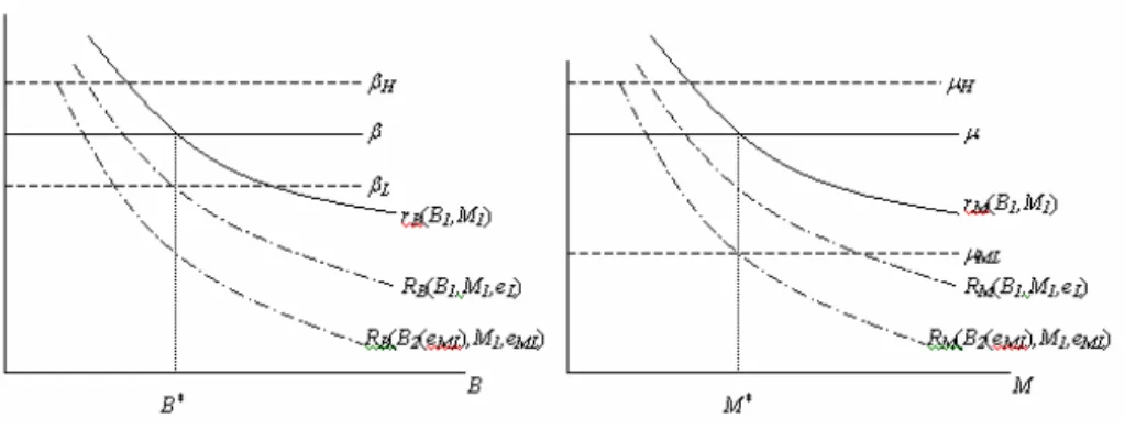
The building-machinery framework is illustrated in 1. First-period prices are given by the solid horizontal linesβandµ. The solid curvesRBandRM describe the first-period marginal return
func-tions of buildings and machines, respectively. The equilibrium capital stock in the first period does not necessarily correspond to the intersection of marginal return and price curves (positionsB∗
and M∗
in the graph).2 Optimal first-period levels are affected by the balance between expandability and
reversibility costs, as well as by the shape of the c.d.f. F(e). The intuition is straightforward. An easily expandable but nearly irreversible project will probably hold a lower level of capital compared to an
2Indeed, this intersection will be the first-period equilibrium only in a particular situation in which opposite forces that affect
easily reversible but nearly non-expandable one.3In addition, if a bad shock is much more likely than a
good shock (if the c.d.f. begins with a sharp increase), first-period capital stock tends to be low.
Figure 1 –Investment Prices and Marginal Revenues
The shock is represented by a shift in the marginal revenue function. A good (bad) shock implies that the marginal revenue curve shifts upward (downward). Figure 1 depicts two bad shocks. The small bad shockeLis represented by a short downward shift of the marginal revenue curves (the upper
dashed curves). If, for convenience, we assume thatB1 =B∗andM1 =M∗, theneL would not be
large enough to induce the firm to disinvest. Marginal returns would still remain at least as large as resale prices. The firm would choose to sell buildings if the shock is larger thaneL. FromeLtoeM L
there is some disinvestment in buildings but not in machinery. The great bad shockeM Lis the edge
of inaction related to the stock of machines. It is represented by a large downward shift of marginal revenue curves. When the shock is worse thaneM L, the second-period marginal return of machines at
the levelM1=M∗is lower than its resale price. In this case, the market conditions become so adverse
that it is desirable to sell machines, in spite of their high reversibility costs.
Summing up, there is a range of inaction for the adjustment of both types of capital in the second period. Nevertheless, the hypothesis of near irreversibility of machines assigns a larger range of inac-tion to their second-period adjustment. Thus, the firm must choose one among four different regimes in period two: disinvestment in machines and buildings, disinvestment only in buildings, inactivity or investment in machines and buildings. If the amount of buildings and machines held by the firm in period one isB1andM1respectively, the expected present value of the flow of returns is given by
V(B1, M1) =r(B1, M1)+
γ
eM L
Z
−∞
{R(B2(e), M2(e), e) + +βL[B1−B2(e)] +µM L[M1−M2(e)]}dF(e)+
γ
eL
Z
eM L
{R(B2(e), M1, e) +βL[B1−B2(e)]}dF(e) +γ eH
Z
eL
R(B1, M1, e)dF(e)+
γ ∞
Z
eH
{R(B2(e), M2(e), e)−βH[B2(e)−B1]−µH[M2(e)−M1]}dF(e) (1)
3This is certainly the case if the equality between first-period prices and marginal returns occurs with the same level of capital
where0 < γ <1is the discount factor. Equation 1 states that the value of the firm,V, corresponds to the sum of expected returns obtained in both periods. The first term in the right-hand side of (1) is the first-period return. The second, third, fourth and fifth terms in the right-hand side of the equation represent the expected value of second-period returns, discounted by the factor γ. This return can be accomplished through each of the four regimes. If e is lower thaneM L, the discounted average
return is given by the second term. The firm wishes to reduce the stock of buildings from B1toB2(e)
and the stock of machines fromM1 toM2(e). The shortening in the second-period return is more
than compensated by the resources from selling buildings,βL[B1−B2(e)], and machines,µL[M1−
M2(e)]. Ifelies betweeneM LandeL, then the firm sells buildings but keeps its first-period stock of
machines. In this case, the average second-period cash flow is represented by the third term on the right-hand side of (1). The fourth term gives the discounted average return with complete inaction. When the shock ranges fromeLtoeH the impact on returns is not large enough to compensate the
reversibility/expandability costs. The firm buys machines and buildings if e > eH. A higher return,
given byR(B2(e), M2(e), e), is obtained at the expenses of the purchase of new buildings,βH[B2(e)−
B1], and new machines,µH[M2(e)−M1].
The representative firm is assumed to maximize the present value of its two-period profits. For that reason, the first-period stock of buildings and machines must be chosen according to the optimization problem given by
M axB1,M1V(B1, M1)−βB1−µM1 (2)
This maximization yields the two following first-order conditions
rB(B1, M1) +γβLF(eL) +γ eH
Z
eL
RB(B1, M1, e)dF(e) +γβH[1−F(eH)] =β (3)
rM(B1, M1) +γµM LF(eM L) +γ eL
Z
eM L
RM(B2(e), M1, e)dF(e)+
γ
eH
Z
eL
RM(B1, M1, e)dF(e) +γµH[1−F(eH)] =µ (4)
These two expressions state that the marginal value of each type of capital in period one should be equal to its respective first-period price. This marginal value is the sum of first-period and expected second-period marginal returns. As we emphasized before, optimal levels of B1and M1depend, among
other things, on the shape of the c.d.f.. If the probabilities are strongly concentrated in low levels ofe, thenF(eL) andF(eM L) are relatively high and[1−F(eH)]is relatively low. As long asβH > βLand
µH > µM L, the equilibrium asserted by equations 3 and 4 hints that the firm chooses low levels ofB1
andM1. Furthermore, it seems intuitive that a high probability of a bad shock in period two induces
the firm to hold a small capital stock in period one. If, otherwise, the probabilities are scarce in low levels ofeand concentrated aboveeH, thenF(eL)andF(eM L)are relatively low and[1− −F(eH)]
is relatively high. A large probability of a good shock in period two implies that the firm expects a high second-period marginal return of capital (since it is assumed thatRM e andRBe are positive).
2.2. Changing Reversibility and Expandability Costs
An interesting exercise is to examine the effect of variations in reversibility and expandability costs on the first-period stock of buildings and machines. To do so, we have to use comparative static multi-pliers. Differentiating expressions (3) and (4) with respect to first-period building and machinery stocks and second-period purchase and resale prices, we obtain
rBBdB1+rBMdM1+γF(eL)dβL+γΓ1dB1+γΓ3dM1+γ[1−F(eH)]dβH= 0 (5)
rM MdM1+rM BdB1+γF(eM L)dµM L+γΓ4dM1+γΓ2dM1+γΓ3dB1+γ[1−F(eH)]dµH = 0 (6)
where theΓ’s are:
Γ1= eH
Z
eL
RBB(B1, M1, e)dF(e)<0
Γ2= eH
Z
eL
RM M(B1, M1, e)dF(e)<0
Γ3= eH
Z
eL
RBM(B1, M1, e)dF(e) = eH
Z
eL
RM B(B1, M1, e)dF(e)>0
Γ4= eH
Z
eM L
RM M(B2(e), M1, e)dF(e)<0
Putting expressions (5) and (6) in a matrix form, we have
rBB+γΓ1 rBM+γΓ3
rM B+γΓ3 rM M+γ(Γ4+ Γ2) . dB1 dM1 = =
−γF(eL) −γ[1−F(eH)] 0 0
0 0 −γF(eM L) −γ[1−F(eH)] . dβL dβH
dµM L
dµH (7)
First-period stocks of buildings and machines are also positively related to their respective purchase prices in period two. It means that when expandability is undermined (when the costs of expanding capital stock in the future increases), then firms will hold a higher stock of capital in the present. By doing this, they partly get rid of incurring large costs to adjust their capital stock in the future to a favorable market change. Once more, cross effects are positive. If there is an increase in the second-period purchasing price of buildings, then firms will raise their first-second-period stock of buildings. Since machines and buildings are complements, the optimal level of the former will also rise.
2.3. The Effect of Uncertainty with Total Irreversibility and Non-expandability
Here we consider a mean-preserving spread, the famous Rothschild and Stiglitz (1970, 1971) char-acterization of an increase in the uncertainty of a distribution. In our setup, we consider a spread in the distribution function of the random shock,f(e), in which the tails become thicker, but the mean is preserved. Hence, the probability of either a very bad or a very good shock increases, but the expected value of the shock remains the same.
We consider the case where the firm has to commit in the second period with the levels of capital acquired in the first period. So investment is completely irreversible and non-expandable. In this case, the value of the firm is given by
V(B1, M1) =r(B1, M1) +γ
∞
Z
−∞
R(B1, M1, e)dF(e) (8)
And the first-order conditions for the profit maximization become
rB(B1, M1) +γ
∞
Z
−∞
RB(B1, M1e)dF(e) =β (9)
rM(B1, M1) +γ
∞
Z
−∞
RM(B1, M1e)dF(e) =µ (10)
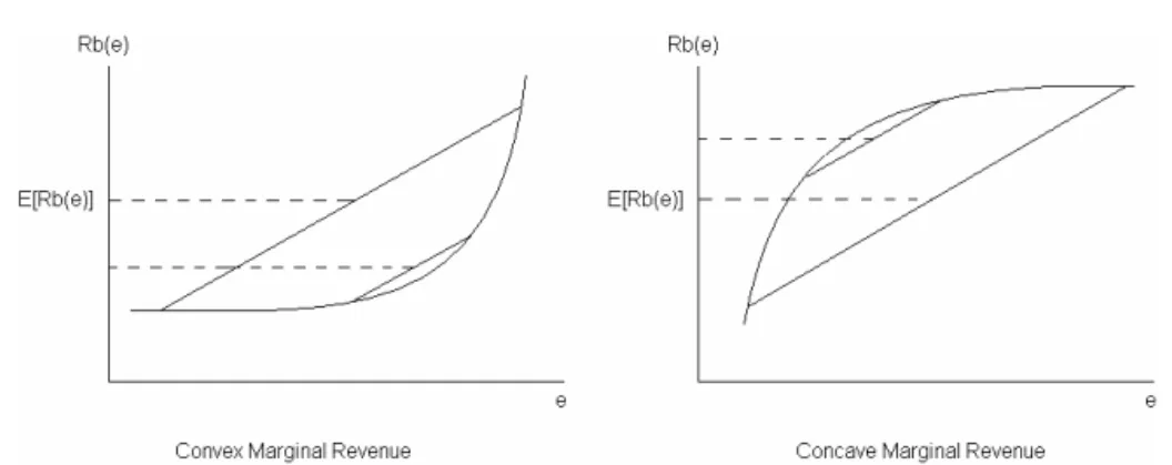
Essentially, what we have here is that the first-period marginal revenue of each input plus the discounted expected value of the second-period marginal revenue has to be made equal to its price. The integrals on the left-hand sides of (9) and (10) are the expected values of second-period marginal revenues. Our interest is on how these expected values will change with a mean-preserving spread in f(e). The effect of uncertainty in the first-period investment will depend on the shapes of functions RB andRM. So far, we imposed the restriction that the shock affects positively marginal revenues (RBeandRM eare both positive). But the effect of uncertainty will depend on the signal of the second
derivatives ofRBandRM with respect to the shocke(see Figure 2).
If marginal revenues are convex one, then more uncertainty raises the expected second-period marginal revenue, and as a consequence induces a higher investment in period one. If, on the other hand, marginal revenues are concave one, then uncertainty hampers investment in period one. By the same token, ifRBandRMare linear one, then uncertainty does not affect investment.
3. EMPIRICAL ASSESSMENT
Figure 2 –A Mean-Preserving Spread
do so, we use a panel of the Brazilian industry spanning the years 1966 to 1995 and comprising 22 industrial sectors (see Appendix 1). The data are mainly drawn from industrial surveys produced by IBGE, which is the Brazilian government institute for statistics.
Our first task is to construct a proxy for uncertainty. A number of empirical studies about the investment-uncertainty relationship adopt sample variability as the indicator of uncertainty. For time-series analysis the typical procedure is to use first differences of aggregate time-series like inflation, real exchange rate or interest rate. Another possibility is to proxy uncertainty by calculating deviations of the time mean for each of these series.
It is worth noting that the empirical literature quite often relies on panel data techniques to study the effects of uncertainty on investment (see, for example, Sérven (1998), Aizenman and Marion (1996), Pindyck and Solimano (1993), among others). When the cross-section dimension is taken into account, uncertainty is usually measured by second moments for each point in time. Volatility indicators may be the standard deviations of aggregate series in the case of cross-country studies, or of company-level variables in the case of individual firms. The intuition behind the use of sample variation as a proxy of uncertainty may be considered incomplete. The idea is that when a variable becomes more volatile, it would be more difficult to make accurate predictions about its future values. Therefore, uncertainty would increase. However, sample variation comprises predictable as well as unpredictable movements of the variable. It is straightforward that uncertainty must mach only the unpredictable component of a variable’s path (since something that is deterministically predicted cannot be uncertain).
A number of studies have adopted more refined measures of uncertainty (see Sérven (1998), Price (1995, 1996) and Pereira (2001)). It is argued that good proxies for uncertainty should be based on the volatility of the variable’s innovations, not on its full volatility. If the variable can be described by a stochastic process, then the usual hypothesis of a constant variance for the error term should be ruled out. This approach leads to the generalized conditional heteroskedastic (GARCH) model, first developed by Bollerslev (1986). In GARCH specifications the conditional variance of the residual is assumed to follow an ARMA process. The use of maximum likelihood techniques allows a simultaneous estimation of an AR process for the variable and an ARMA process for the conditional variance of the error term. Uncertainty is given by the fitted values of this conditional variance. We follow this GARCH-based approach, selecting two variables to be examined: the aggregated industrial value and the average earnings (which we just call wages). Thus, two uncertainty series are obtained for each of the twenty-two industrial sectors, generating twenty-two uncertainty panels. The following univariate GARCH is estimated sector by sector separately
hi,t=ci+diµ 2
i,t−1+eihi,t−1 (12)
where: i = 1,2, ...,22andt = 1,2, ...,30;y is the selected variable (wages or aggregated value by industry); andhi,t is the variance ofµi,t conditional on information available in periodt. We also
estimate two more uncertainty panels based on the same GARCH(1,1)model, but excluding the constant and/or the trend in the AR equation whenever they are not significant at the 5% level.
In addition to the two uncertainty panels, we estimate for the inflation and the interest rate the same univariated GARCH(1,1) given by (11) and (12). That gives us two additional uncertainty series. However, unlike wages and production, these are not sector specific. They vary over time, but not across sectors. We obtain a single time series for inflation uncertainty and a single time series for interest rate uncertainty. In a panel data context, these work as time dummies, capturing the effect of a particular year over all the twenty two sectors.
As long as the time dimension spans only 30 years of annual data, we do not have many degrees of freedom in the estimation of the GARCH. For example, in the full setup with constant and trend given by equations 11 and 12, we would be left with only 24 degrees of freedom. Hence, we did not pursue more complex auto-regressive specifications, in which the lack of degrees of freedom would become a serious issue. We just used the parsimoniousGARCH(1,1). Since the original work of Bollerslev (1986), a number variations of the GARCH model have been developed. There are nowadays in the literature at least twelve variants of the GARCH model. Some of them imply the lost of degrees of freedom, some of them do not. To name a few, the EGARCH (exponential general autoregressive conditional heterskedas-tic) model has the conditional variance expressed in logs. The QGARCH (quadratic GARCH) adds to the conditional variance equation 12 in the case of ourGARCH(1,1)) non-quadratic lags of the errorµ, allowing one to capture eventual asymmetries between positive and negative shocks. The GARCH-M (GARCH-in-mean) adds a conditional variance term in the mean equation. In spite of this variety, the bulk of the literature on economic uncertainty has still been using the simpleGARCH(1,1)structure to model economic uncertainty (see, for example, Conin and Kennedy (2007), and Atta-Mensah (2004)).
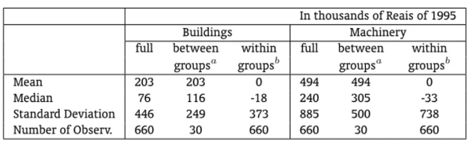
Before analyzing the investment-uncertainty relationship for the Brazilian industry it is worth look-ing at some descriptive statistics of our investment panel. Table 1 presents this basic information separately for the investment in buildings and in machinery. The mean, median and standard deviation are calculated for the full sample, for the sector averages (between groups), and for the deviations of respective group means (within groups). This latest option puts away the variation related to sector particularities (since sector means are supposedly different for different sectors), allowing the analysis of the time-series dimension. Table 1 reveals at least three important aspects. First, medians are always smaller than means, which implies that frequency distributions are positively skewed in both time-series and cross-section dimensions. Accordingly, distributions have lower frequencies in their upper tails, suggesting that large levels of investment are concentrated in some few years and sectors. The second point is that variation is higher over time than across sectors in both types of investment. This result reinforces the stylized fact of the non-smoothness of investment over time in disaggregated se-ries.4The kinky path is a consequence of the irreversible nature of investment, which produces a range
of inaction and a profitability threshold. Investment projects are performed only when the expected future profitability exceeds this threshold. A third feature is the fact that investment in machinery is much more volatile than investment in buildings, in a proportion of nearly two to one.
We have seen in the model that, in the case of a bad shock, capital in the form of buildings would be firstly sold due to a lower reversibility cost. The question is, shouldn’t we expect a higher volatility of investment in industrial real estate, rather than in machinery? These aspects might not be
contra-4This is specially valid for disaggregated investment. It is quite obvious that periods of positive investment are imperfectly
Table 1 –Descriptive Statistics of Investment in Brazil
In thousands of Reais of 1995
Buildings Machinery
full between within full between within groupsa groupsb groupsa groupsb
Mean 203 203 0 494 494 0
Median 76 116 -18 240 305 -33
Standard Deviation 446 249 373 885 500 738
Number of Observ. 660 30 660 660 30 660
aSector averages.
bDeviations from sector averages.
dictory if we think that machines depreciate faster than real estate. Hence the cycle of reinvestment should take place more often for machines than for buildings.
To investigate how private investment in machinery and in real estate are affected by uncertainty, we use a conventional empirical equation that relates investment to uncertainty measures and to a set of variables typically used to describe investment. Besides the GARCH-based uncertainty proxies, we use three other variables in the empirical specification: aggregated industrial value, interest rates and inflation. The first one should capture the effects of economic activity on the investing decision.5
Investment tends to be higher in periods of high production and high capacity utilization.
While aggregate industrial value is obtained from a pooled sample, interest rates and inflation are macroeconomic variables that vary over time, but not across sectors. When their values are replicated to each sector they actually work as time dummies. Interest rates are the standard measure of the user cost of capital. The larger is the opportunity cost of investing, proxied by the interest rate, the less attractive is investment. The data for interest rates in Brazil are usually available in high frequency series (like daily or weekly rates). This kind of information has the inconvenience of covering small time spans. To put this problem aside, we use the return of CDB bonds (certificado de depósitos bancários). Prior to 1970, however, these data are not available. The missing values are then fulfilled with the return offered by a federal public bond named ORTN (obrigações reajustáveis do tesouro nacional).
The data for inflation is based on the IGP-DI (índice geral de preços – disponibilidade interna), a widely used price index in Brazil. Inflation is employed essentially as a control variable that corrects an undesirable feature of PIA data set (see Appendix 1). It is also important to account for the dynamics of investment. Current changes in the capital stock likely depend on past changes. Some kind of inertia may be present, especially with annual data. Therefore, we also included lagged investment among the regressors. The equation to be estimated is given by:
Ii,t =θIi,t−1+fi+β1Ui,t1 +β2Ui,t2 +β3yi,t+β4rt+β5πt+β6Utπ+β7Utr+ǫi,t (13)
where: Iis investment in machines or in buildings; U1
is the uncertainty proxy based on the value aggregated by industry; U2
is the uncertainty proxy based on wages;y is the aggregated industrial value; ris the interest rate;πis inflationUπ is the uncertainty proxy based on inflation;Ur is the
uncertainty proxy based on interest rates; and ǫis the random disturbance. Thefiterm is a sector
specific constant in the case of fixed effects approach, or a sector specific disturbance in a random effects estimation.
The problems of random effects techniques have been increasingly recognized in the literature. The main drawback is the likely correlation of individual effects with the observed exogenous variables.
5The use of production variables in investment equations usually brings about problems of endogeneity. If strong exogeneity of
For example, an industrial sector that faces highly unionized workers should have high wage-related uncertainty levels. If the degree of unionization is considered as an individual effect, and if this effect is treated as a random error, then the consistency hypothesis are clearly violated in the regression model. An alternative is to estimate (13) by the fixed effects method. However, since the work of Nickell (1981), it has been largely pointed out that the fixed effects model estimated by OLS contains serious problems of bias when lags of the dependent variable are included in the regressors. The use of instrumental variable procedures is the standard way to tackle these problems as well as problems of endogeneity of the production variabley(see footnote 5). However, instead of performing fixed effects estimation, we take first differences of (13) in order to remove individual effects:6
∆Ii,t=θ∆Ii,t−1+β1∆Ui,t1 +β2∆Ui,t2 +β3∆yi,t+β4∆rt+β5∆πt+
β6∆Utπ+β7∆Utr+ui,t (14)
where:ui,t=ǫi,t−ǫi,t−1. Instrumental variables are required to put aside problems of endogeneity of
regressors and of correlation between the lagged difference of the dependent variable and the residuals ui,t.7 Second- and higher-order lags of the endogenous variable can be used as instruments (see
Arel-lano and Bond (1991)). The use of these instruments is based on the fact thatE[∆Ii,t−2∆Ii,t−1]6= 0
andE[∆Ii,t−2ui,t] = 0. Yet, this latest equality requires serially uncorrelated residuals.8
Before the empirical implementation of (14), an important aspect of the data should be regarded. Instead of total sector investment, we take the average investment of one firm in that sector (see again Appendix 1). The choice of a variable sample in the data assembling methodology prevents the use of total values and leads to grouped data methods. Specifically, repeated cross-sections can be used as a pseudo-panel model that looks like a standard model of panel data (see, for example, Deaton (1985), and Menezes-Filho et al. (2000).
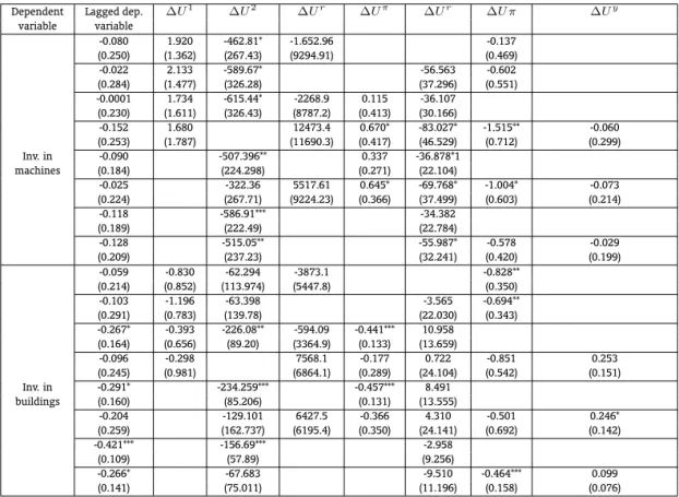
The results of the instrumental variables estimation of (14) are presented in Table 2. The first part of the table reports the estimates of investment in machines, while the second part refers to investment in buildings.9The lags from two to twelve of the dependent variable are used as instruments.
The first column of Table 2 shows that investment is always negatively related to its previous value. However, statistical significance at the conventional levels is obtained only for buildings. Intuitively, if a firm acquired a new building last year, there is probably no need for purchasing new buildings this year. The coefficients of the interest rate have the expected negative sign for most of the regressions of machines and buildings as well. A high interest rate tends to depress both types of investment, since it is closely related to the opportunity cost of capital. These estimates, however, are not highly significant. The 10% level of significance is reached only in few regressions.
Each regression in Table 2 is performed with a different set of regressors. The same regression is run with the investment in machines and in buildings. So we can compare the results of each regression in the upper part of the table with the corresponding regression in the lower part of the table. The role of inflation is to control for one imperfection of the database. We have seen that our data set tends to underreport real investment in periods of high increases in price levels. Therefore, the estimated coeffi-cients of inflation in Table 2 have the expected sign. It should be noted, however, that investment and
6More detail of this approach can be found in Sérven (1998) or in Arellano and Bond (1991).
7In this respect, it can be seen that E[∆I
i,t−1ui,t] = E[(Ii,t−1 −Ii,t−2)(ǫi,t−ǫi,t−1)] = E(Ii,t−1ǫi,t−1) =
E(ǫ2
i,t−1)6= 0. Thus, the use of OLS in (11) does not yield unbiased and consistent estimates of parameters.
8For instance, ifǫ
i,tfollows an AR(1) process likeǫi,t=ρǫi,t−1+ψi,t, then:E[∆Ii,t−2ui,t] =−ρE[Ii,t−2ǫi,t−2]6= 0.
In this case, the second-order lag of the endogenous variable would not be a valid instrument.
9Besides our two key uncertainty measuresU1andU2, we also tried proxies constructed with the same GARCH(1,1) model,
inflation are negatively related not only because an inflationary environment harms capital profitabil-ity, but also because the methodology of gathering data yields underreported values when inflation is high. The levels of significance for the inflation (∆π) coefficient vary through the regressions. They are significant at the 10% level on half of the regressions reported in Table 2. The value aggregated by industry is negatively related with investment in machines, contrarily to theoretical predictions, and positively related with investment in buildings. Yet, they tend to be non-significant at the conventional levels.
The most interesting aspect of Table 2 is the uncertainty coefficients estimates. The second column of the table (∆U1
) suggests that uncertainty related to production does not exert a significant influence on both categories of investment. Nevertheless, uncertainty related to wages has large and, in many cases, highly significant coefficients, as can be seen in the third column of the table (∆U2
). The results provide empirical support to the main assertion of the model presented in section 2, namely the idea that uncertainty has a larger impact on investment in machinery compared to investment in real estate, because of the less reversible nature of the former. It should be noted that coefficients for wage-related uncertainty are always higher, in absolute values, when investment in machinery is the dependent variable. The estimates ofβ2are from 2.1 to 9.3 times larger in the upper portion than in the down
portion of the table. This empirical finding suggests that uncertainty affects investment in machinery more intensely than investment in buildings.
Table 2 –Pooled Instrumental Variables Estimation of the Investment Equation
Dependent Lagged dep. ∆U1 ∆U2 ∆Ur ∆Uπ ∆Ur ∆U π ∆Uy
variable variable
-0.080 1.920 -462.81* -1.652.96 -0.137 (0.250) (1.362) (267.43) (9294.91) (0.469) -0.022 2.133 -589.67* -56.563 -0.602 (0.284) (1.477) (326.28) (37.296) (0.551) -0.0001 1.734 -615.44* -2268.9 0.115 -36.107
(0.230) (1.611) (326.43) (8787.2) (0.413) (30.166)
-0.152 1.680 12473.4 0.670* -83.027* -1.515** -0.060 (0.253) (1.787) (11690.3) (0.417) (46.529) (0.712) (0.299) Inv. in -0.090 -507.396** 0.337 -36.878*1
machines (0.184) (224.298) (0.271) (22.104)
-0.025 -322.36 5517.61 0.645* -69.768* -1.004* -0.073 (0.224) (267.71) (9224.23) (0.366) (37.499) (0.603) (0.214)
-0.118 -586.91*** -34.382 (0.189) (222.49) (22.784)
-0.128 -515.05** -55.987* -0.578 -0.029 (0.209) (237.23) (32.241) (0.420) (0.199)
-0.059 -0.830 -62.294 -3873.1 -0.828** (0.214) (0.852) (113.974) (5447.8) (0.350) -0.103 -1.196 -63.398 -3.565 -0.694** (0.291) (0.783) (139.78) (22.030) (0.343) -0.267* -0.393 -226.08** -594.09 -0.441*** 10.958
(0.164) (0.656) (89.20) (3364.9) (0.133) (13.659)
-0.096 -0.298 7568.1 -0.177 0.722 -0.851 0.253 (0.245) (0.981) (6864.1) (0.289) (24.104) (0.542) (0.151) Inv. in -0.291* -234.259*** -0.457*** 8.491
buildings (0.160) (85.206) (0.131) (13.555)
-0.204 -129.101 6427.5 -0.366 4.310 -0.501 0.246* (0.259) (162.737) (6195.4) (0.350) (24.141) (0.692) (0.142) -0.421*** -156.69*** -2.958
(0.109) (57.89) (9.256)
-0.266* -67.683 -9.510 -0.464*** 0.099 (0.141) (75.011) (11.196) (0.158) (0.076) Notes: The simbols ***, ** and * are used to indicate significance at 1%, 5% and 10%, respectively. Standard errors are in brackets. The set of instruments is compounded of the lags from 2 to 12 of the dependent variable taken in first differences. Hereris the interest ratepis the inflation rate,yis the value aggregated by the industry, andU1,U2,UrandUπare, respectively, production, wages, interest rate and inflation-related uncertainty proxies.
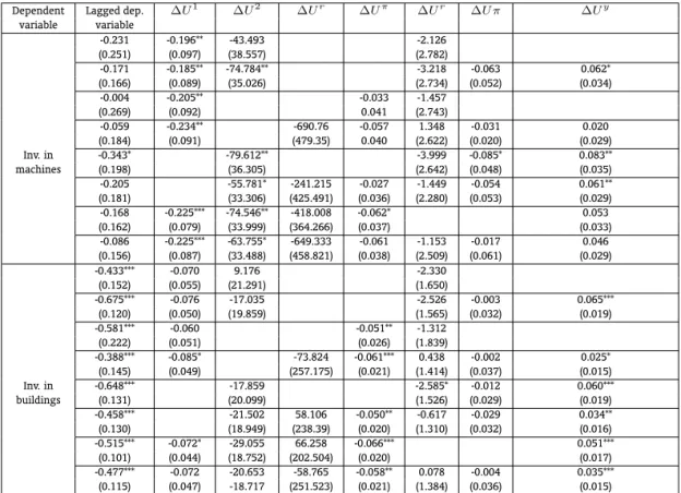
lags from one to six of the independent variables used in each estimation (not including the lags of the lagged dependent variable). The results are presented in Table 3. Unlike Table 2 , each regression in Ta-ble 3 has a different set of instruments. The results are not much different from those of TaTa-ble 2. Once more, investment is negatively related to its lagged values. Yet, statistical significance is considerably higher for buildings. The estimates for the interest rate coefficients are not significant at the conven-tional levels, but they reinforce the expected negative relationship among investment and the user cost of capital. Table 3 also reports negative coefficients for inflation, which is in line with our previous find-ings, and positive and in some cases highly significant coefficients for the value aggregated by industry. Hence, investment tends to happen in sectors and years where production is large. Most importantly, uncertainty coefficients are again much higher for machines than for buildings. However, differently from the results in Table 2, investment in machines is significantly affected by both production- and wage-related uncertainty. Investment in buildings, on the other hand, have much smaller and generally non-significant uncertainty coefficients. The effect of inflation uncertainty is slightly more intense on investment in buildings than on machinery. We did not find statistical significance for the interest rate uncertainty coefficient in any of the regressions performed in Table 3. In a broad sense, it can be said that Table 3 replicates the main results of Table 2.
Table 3 –Pooled Instrumental Variables Estimation of the Investment Equation with a Different Set of Instruments
Dependent Lagged dep. ∆U1 ∆U2 ∆Ur ∆Uπ ∆Ur ∆U π ∆Uy
variable variable
-0.231 -0.196** -43.493 -2.126 (0.251) (0.097) (38.557) (2.782)
-0.171 -0.185** -74.784** -3.218 -0.063 0.062* (0.166) (0.089) (35.026) (2.734) (0.052) (0.034)
-0.004 -0.205** -0.033 -1.457 (0.269) (0.092) 0.041 (2.743)
-0.059 -0.234** -690.76 -0.057 1.348 -0.031 0.020 (0.184) (0.091) (479.35) 0.040 (2.622) (0.020) (0.029) Inv. in -0.343* -79.612** -3.999 -0.085* 0.083** machines (0.198) (36.305) (2.642) (0.048) (0.035) -0.205 -55.781* -241.215 -0.027 -1.449 -0.054 0.061** (0.181) (33.306) (425.491) (0.036) (2.280) (0.053) (0.029) -0.168 -0.225*** -74.546** -418.008 -0.062* 0.053 (0.162) (0.079) (33.999) (364.266) (0.037) (0.033) -0.086 -0.225*** -63.755* -649.333 -0.061 -1.153 -0.017 0.046 (0.156) (0.087) (33.488) (458.821) (0.038) (2.509) (0.061) (0.029) -0.433*** -0.070 9.176 -2.330
(0.152) (0.055) (21.291) (1.650)
-0.675*** -0.076 -17.035 -2.526 -0.003 0.065*** (0.120) (0.050) (19.859) (1.565) (0.032) (0.019) -0.581*** -0.060 -0.051** -1.312
(0.222) (0.051) (0.026) (1.839)
-0.388*** -0.085* -73.824 -0.061*** 0.438 -0.002 0.025* (0.145) (0.049) (257.175) (0.021) (1.414) (0.037) (0.015) Inv. in -0.648*** -17.859 -2.585* -0.012 0.060*** buildings (0.131) (20.099) (1.526) (0.029) (0.019) -0.458*** -21.502 58.106 -0.050** -0.617 -0.029 0.034** (0.130) (18.949) (238.39) (0.020) (1.310) (0.032) (0.016) -0.515*** -0.072* -29.055 66.258 -0.066*** 0.051*** (0.101) (0.044) (18.752) (202.504) (0.020) (0.017) -0.477*** -0.072 -20.653 -58.765 -0.058** 0.078 -0.004 0.035*** (0.115) (0.047) -18.717 (251.523) (0.021) (1.384) (0.036) (0.015) Notes: The simbols ***, ** and * are used to indicate significance at 1%, 5% and 10%, respectively. Standard errors are in brackets. The set of instruments is compounded of the lags from 1 to 6 of the independent variable taken in first differences (not including the lags of the lagged dependent variable). Hereris the interest ratepis the inflation rate,yis the value aggregated by the industry, andU1,
U2,Ur
andUπare, respectively, production, wages, interest rate and inflation-related uncertainty proxies.
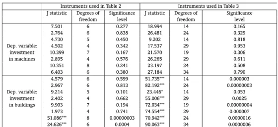
exogene-ity of the instruments seems to be a particularly common problem in regressions with instrumental variables. Even though we are using lagged values as instruments, in the tradition of dynamic panel estimation, we have to ascertain that they are indeed exogenous. Hence we perform a test for over-identifying restrictions. We use here a J-test. Basically, we estimate the equation 14 using instrumental variables. Then we regress the computed residuals on the instruments. We compute the F-statistic of the latter regression from testing that all the coefficients are jointly zero. We hence compute the over-identifying restriction test statistic, which is given byJ=mF, where m is the number of instruments. The test statistic is distributed as Qui-square withm−rdegrees of freedom, where r is the number of endogenous variables.
The results of the test for overidentifying restrictions are reported on Table 4. The lags 2 to 12 of the dependent variable seem to be good instruments for most of the regressions of Table 2. The only exceptions are the last 2 ones with investment in buildings as the dependent variable. In the majority of cases, theJ test generates statistics that are non-significant at the conventional levels, indicating that the instruments are indeed exogenous, solving the problem of endogenous regressors. Hence the key result of Table 2 is valid, and for 14 out 16 regressions performed we can conclude that our instrumental variables estimators are consistent. The results are not that straightforward in Table 3. When we use the lags 1 to 6 of the regressors as instruments, they do not solve the endogeneity problem in the bottom half of the table (when investment in buildings is the endogenous variable). Hence the instrumental variables estimators might not be consistent due to the potential endogeneity of some regressors. In this case, our comparison of uncertainty effects might be compromised. In spite of that, our results provide good evidence that the investment in the form of machines tends to suffer more from economic uncertainty (especially wage-related uncertainty) than the investment in the form of buildings and real estate in general.
Table 4 –J-test for Overidentifying Restrictions
Instruments used in Table 2 Instruments used in Table 3 J statistic Degrees of Significance J statistic Degrees of Significance
freedom level freedom level 7.501 6 0.277 18.994 14 0.165 2.764 6 0.838 26.481 24 0.329 4.730 5 0.450 9.202 14 0.818 Dep. variable: 4.502 4 0.342 17.537 29 0.953 investment 10.399 7 0.167 21.570 19 0.306 in machines 2.895 4 0.576 26.265 29 0.611 10.351 8 0.241 23.197 24 0.508 6.403 6 0.380 27.184 34 0.790 4.579 6 0.599 51.735*** 14 0.000003 2.967 6 0.813 82.192*** 24 0.00000003 Dep. variable: 9.214 5 0.101 23.446* 14 0.053
investment 2.402 4 0.662 55.006*** 29 0.0025 in buildings 9.903 7 0.194 72.034*** 19 0.00000004
1.973 4 0.741 74.554*** 29 0.000007 51.086*** 8 0.00000003 70.942*** 24 0.0000016 24.626*** 6 0.0004 90.063*** 34 0.0000006 Notes: The simbols ***, ** and * are used to indicate significance at 1%, 5% and 10%, respectively. For Table 2, the set of instruments is compounded of the lags from 2 to 12 of the dependent variable taken in first differences. For Table 3, the set of instruments is compounded of the lags from 1 to 6 of the independent variables taken in first differences (not including the lags of the lagged dependent variable).
4. CONCLUDING REMARKS
react to conventional variables in the same way. Specifically, if the expansion in capacity is concentrated in an easily expandable but nearly irreversible good, uncertainty reduces the incentive to invest. If, otherwise, the project is based on a non-expandable but easily reversible input, uncertainty tends to accelerate investment.
This paper decomposes investment in industrial real estate and machinery. The main concern is to analyze how each of these components is affected by uncertainty. The existing theoretical analysis suggests, in large part, the presence of opposing effects, which means that the sign of the investment-uncertainty relation can be assessed only empirically. In this regard, the paper performs an empirical investigation using Brazilian industry data. Instead of calculating naive measures of uncertainty, we construct more refined proxies based on the volatility of the innovations to two key variables: aggre-gated industrial value and average wages. We also construct proxies based on inflation and interest rates. But since these vary through time but not across sectors, they work as time dummies. We then focus our attention on the uncertainty panels associated with production and wages.
Bibliography
Abel, A. (1983). Optimal investment under uncertainty. American Economic Review, 73(1).
Abel, A., Dixit, A., Ebelry, J., & Pindyck, R. (1996). Options, the value of capital, and investment. The Quarterly Journal of Economics, 111(3).
Aizenman, J. & Marion, N. (1996). Volatility and the investment response. Technical Report WP 5841, NBER.
Arellano, M. & Bond, S. (1991). Some tests of specification for panel data: Monte Carlo evidence and an application to employment equations. Review of Economic Studies, 58.
Atta-Mensah, J. (2004). Money demand and economic uncertainty. Technical Report 2004-25, Bank of Canada.
Bertola, G. & Caballero, R. (1994). Irreversibility and aggregate investment. Review of Economic Studies, 61.
Bollerslev, T. (1986). Generalized autoregressive conditional heteroskedasticity. Journal of Econometrics, 31.
Caballero, R. (1991). On the sign of the investment-uncertainty relationship.American Economic Review, 81(1).
Campa, J. & Goldberg, L. (1993). Investment in manufacturing, exchange-rates and external exposure. Technical Report 4378, NBER.
Carruth, D. & Henley, A. (1999). What do we know about investment under uncertainty? Journal of Economic Surveys (forthcoming).
Conin, D. & Kennedy, B. (2007). Does uncertainty impact money growth? A multivariate GARCH analy-sis. Technical Report Research Technical Paper 6RT07, Central Bank & Financial Services Authority of Ireland.
Cruz, B. & Pommeret, A. (2006). Irreversible investment with embodied technological progress. Technical Report 1171, IPEA.
Deaton, A. (1985). Panel data from time series of cross-sections.Journal of Econometrics, 30.
Henley, A. (1999). Does uncertainty accelerate or retard investment? Panel data evidence. In Teixeira, J. & Carneiro, F., editors,Proceedings of the II International Colloquium on Economic Dynamics and Economic Policy, Brasília.
Menezes-Filho, N., Azzoni, C., Menezes, T., & Silveira-Neto, R. (2000). Convergence with MicroData: The case of states of Brazil. Technical report, University of São Paulo. unpublished manuscript.
Nickell, S. (1981). Biases in dynamic models with fixed effects. Econometrica, 49(6).
Pereira, R. (2001). Investment and uncertainty in a quadratic adjustment cost model: Evidence from Brazil.Revista Brasileira de Economia, 55(2).
Pindyck, R. (1988). Irreversible investment, capacity choice, and the value of the firm.American Economic Review, 78(5).
Price, S. (1995). Aggregate uncertainty, capacity utilization and manufacturing investment. Applied Economics, 27.
Price, S. (1996). Aggregate uncertainty, investment and asymmetric adjustment in the UK manufactur-ing sector.Applied Economics, 28.
Rothschild, M. & Stiglitz, J. (1970). Increasing risk I: A definition. Journal of Economic Theory, 2(3):255– 243.
Rothschild, M. & Stiglitz, J. (1971). Increasing risk II: Its economic consequences. Journal of Economic Theory, 3(1):66–84.
A. APPENDIX 1
This appendix presents some features and definitions of the data used in the econometric section of the paper. The investigation is based on a panel of Brazilian industries with yearly observations and a set of twenty-two industrial sectors (one mining and twenty-one manufacturing sectors). We use the following arrangement: mineral extraction; nonmetallic minerals; metallurgy; mechanics; electric and communications equipment; transportation equipment; wood; furniture; paper and cardboard; rubber; leather and hides; chemicals; pharmaceuticals; perfumes, soaps and candles; plastics; textiles; clothing, footwear and clothing goods; food products; beverages; tobacco; printing; and miscellaneous.
The raw data is essentially extracted from PIA (Pesquisa Industrial Anual), which is a yearly indus-trial survey produced by IBGE (Instituto Brasileiro de Geografia e Estatística), the Brazilian government institute for statistics. We also use IBGE’s Industrial Census, that takes the place of PIA in 1975, 1980 and 1985.
The main variable in the analysis is investment. PIA has information about the acquisition as well as the sale of production goods for each of the twenty-two industry classes. These goods are split into two main groups. The first one embraces machines, equipment, appliances, vehicles and furniture. The second group refers to real estate, specifically, buildings, land and other landed properties. In order to obtain the average purchase and average sale in each sector, total purchases and sales are divided by the number of informant firms (otherwise, the values would be sensitive to the number of firms in the sample, which varies across the years and sectors). We define investment (or net investment) as the average purchase minus the average sale.
Three more variables are used in order to construct two proxies for uncertainty. The first proxy is based on the aggregated industrial value. Once more, we obtain the average aggregated industrial value through the ratio of the raw information and the number of informant firms. The second proxy is based on the average earnings of occupied people (comprising all kinds of wages and earnings as well as social charges), which is obtained as follows
AEOPj,t=
OEW Ej,t/N IFj,t′
OPj,t/N IFj,t′′
whereOEW Ej,tis the overall expenses on wages and other earnings of sectorjat the timet, with
the respective number of informant firms given byN IF′
j,t, andOPj,tis the occupied people of sector
jat the timet, with the respective number of informant firms given by
N IF′′
j,t
The value in the numerator is the average labor expenses and the value in the denominator is the average occupied people.
Our time span goes from 1966 to 1995. The sample, however, is not complete. In 1971 and 1991 PIA was not performed. Moreover, the sale of production goods and the aggregated industrial value were not reported, respectively, by the 1970’s industrial census and by the 1986/87’s PIA. Since some of the econometric procedures used require continuous samples, we choose an arbitrary method to fulfill the missing values. We estimate an ARMA process with the unavailable data being fulfilled by interpolation (average between the previous and the subsequent value). Fitted values are then used to complete the missing periods.
Monetary values are deflated by IPA-DI (índice de preços por atacado – disponibilidade interna), which is the main wholesale price index in country-regioncountry-regionBrazil. A better strategy would be to use more specific price indexes, for instance, in the case of wages. Nevertheless, none of these indexes are available for the entire time span used in the analysis.
basis (which implies that nominal values in the beginning and in the end of the year are summed and then reported to IBGE). With low levels of inflation this effect can be ignored, but in a highly inflationary environment, the quality of the data might be an issue.