1.Instituto Nacional de Pesquisas Espaciais – Coordenação de Engenharia e Tecnologia Espacial – Divisão de Sistemas Espaciais – São José dos Campos/SP – Brazil. Correspondence author: Sérgio Luís de Andrade Silva | Instituto Nacional de Pesquisas Espaciais – Coordenação de Engenharia e Tecnologia Espacial – Divisão de Sistemas Espaciais | Av. dos Astronautas, 1758 | CEP: 12.227-010 – São José dos Campos/SP – Brazi | E-mail: [email protected]
Received: Mar. 30, 2017 | Accepted: Dec. 19, 2017 Section Editor:Adiel Almeida
ABSTRACT: In the last 50 years, Stakeholder (STH) theory has become one of the main instruments of analysis, identification, classification and management of entities in the complex and conflicting corporate environment. In a similar way, System Dynamics (SD) methodology has been used as an instrument for modeling and simulating the dynamics of complex systems in several areas of knowledge, such as engineering, management, environmental research, health, etc. The main objective of this work is to study the potential of combining these two approaches into a new methodology for modeling, analysis and simulation of organizational complex systems that could aid in the decision-making process. Motivated by social, technological, political and economic challenges observed in the Brazilian Space Program (PEB), the authors use it as a case study for the application of that new methodology. This preliminary study identifies possible cells and molecules of the functional structure of PEB, their interfaces and interactions. It is hoped that the present work would be helpful for later developments in PEBs dynamic modeling and planning.
KEYWORDS: System modeling, Stakeholder theory, System dynamics methodology, Brazilian Space Program.
INTRODUCTION
From a global point of view, it can be considered that space exploration has been following a long and productive path since the launch of the first artificial satellite about 60 years ago. There is currently an intense mobilization by international space agencies, so that the space programs of their countries can be adjusted to the demands, technologies, resources and opportunities of an increasingly globalized world (Bochinger 2008; OECD 2014). More specifically, there are efforts to define, characterize, remodel
and improve the institutional frameworks that shape and support space programs (Fisk 2008; Petroni et al. 2009; SAI 2016). This
set of values and interests, commercial or public nature, can be seen as the business of space programs.
Historically, the Brazilian Space Program (Programa Espacial Brasileiro – PEB) has been serving as an agent of mobilizing resources, able to materialize, even if partially, public policies aimed at strengthening a national scientific and applications space community, achieve technological independency and a sustainable space industry (Costa Filho 2002; Escada 2005; Ribeiro 2007; Pereira 2009). Concerning these last two aspects of PEB, though the Brazilian space industry has already being capable of generating products with high technological content (Oliveira 2014), it is still in an early stage of development, and its consolidation was given high priority by the Brazilian Space Agency (Agência Espacial Brasileira – AEB) (AEB 2012).
Towards the Brazilian Space Program Modeling
Through the Combination of Stakeholder Theory
and System Dynamics Methodology
Sérgio Luís de Andrade Silva1, Fabiano Luís de Sousa1
Silva SLA; De Sousa FL (2018) Towards the Brazilian Space Program Modeling Through the Combination of Stakeholder Theory and System Dynamics Methodology. J Aerosp Technol Manag, 10: e4818. doi: 10.5028/jatm.v10.960.
How to cite
The discrepancy between the Brazilian space program long standing history and ambitions, and PEB’s current size and accomplishments, has motivated many studies to characterize the program, diagnose the roots behind its underdeveloped potential, and suggest possible roadmaps for its expansion. On these matters, it is worth reading the reports on PEB sponsored by the Brazilian Congress (Câmara dos Deputados 2010), the government’s Secretary for Strategic Affairs (SAE 2011), the Brazilian Aerospace Association (AAB 2010) and by the Brazilian Federal Court of Accounts (TCU 2016). Moltz (2015) summarized the hurdles PEB have been encountering through time, pointing out that “the nation’s ability to build a sustainable strategy poses the most significant challenge for Brazil”, in reaching the country’s ambition on space. Certainly, such a strategy should be heavily based on the interests of PEB’s stakeholders.
Stakeholder analysis has been used as a framework to identify actors, even potential ones, which could affect or be affected
by acts of an organization (Laplume et al. 2008). Understanding and taking in account the interests and influence of all of its
stakeholders could provide the organization leadership a better strategic view on the “forces” acting on the makings that lead to successful endeavors, and hence to the organization’s survivor in the long term. Stakeholder analysis is today a common tool in
management practice (Lozano et al. 2015), being used as part of strategic assessments in many fields, including space (Rebentisch
et al. 2005; Sutherland et al. 2012; Oliveira and Perondi 2012). Though stakeholder theory is a very helpful tool for portrait the
organization’s environment in respect to its social and economic ties, it has a limited capacity on capturing the dynamics of such
relationships (Lozano et al. 2015; Friedman and Miles 2002; Miles 2017), which in turn impacts its capacity of forecasting the
possible evolutions of the system.
Understanding system behavior is in the core of a broad area of management modeling and simulation, called system dynamics (Richardson 2011). Based on the concepts of servomechanisms engineering, it is essentially an approach to model and simulate the behavior of complex social systems, in such a way to uncover the internal mechanisms powering their dynamics, and forecast possible system outcomes, in a way to “guide policy and decision making” (Richardson 2011). System dynamics could then provide stakeholder theory a means to overcome its limitation in respect to portrait dynamic behaviors of social and business
ecosystems. In fact, linking STH theory to SD has already been suggested by Elias et al. (2000) as an opportunity for research.
Recently, some authors such as Elias (2012), Inam et al. (2015), Lu et al. (2017), Zaini et al. (2015) and Zwikael et al. (2012), have
proposed particular ways of combining STH and SD. The purpose of all that five articles (as well as the present one) is to use STH theory and SD methodology to model a problem situation and through simulations to analyze and manage a system behavior (and/or its resources).
In other words, each article proposes a different way of making the link between STH and SD and modeling a particular system. For
example, in Table 1 of Elias (2012) and Figure 2 of Zwikael et al. (2012), the authors suggest a specific framework where the main STHs
of a given system are identified and after that, the elements of SD methodology, Causal Loop Diagrams (CLDs) and the Stock and Flow
diagrams (SFDs), are created. Inam et al. (2015), Lu et al. (2017) and Zaini et al. (2015) do not specifically propose a framework, but
follow a similar methodology by mapping the most relevant system STHs, their problems and possible solutions, and then producing the CLD and SFD. The differential of this workflow is the “binding table” where STHs are classified, according to the attributes (power legitimacy and urgency) and their main activities are listed. Based on that list, the elements of SD modeling (variables, flows and stocks) are proposed to best represent each STH activity. Finally the workflow is completed by doing the CLD and SFD. It can be said that one of the most significant contribution here is the clarity and objectivity of the “binding table” which in the last analysis is the instrument that links STH and SD, i.e., it allows making the transition from the STH world to the SD world. In other words, the table shows how to build a CLD (SD world) starting from the most relevant STHs of the system and the main activities performed by them (STH world).
THEORY REVIEW
STAKEHOLDER THEORY
The first studies considering the influence of stakeholders in corporations were published in the 1960s and 1970s. Although at that time there was not a theory about stakeholders, the academy took its first steps to explain and understand old issues due to interactions, expectations and behavior of relations between them, trying to answer questions like: 1) What were the elements that supported the existence of corporations? 2) What was the real purpose of corporations (core business)? and 3) What were and how were formed the dependency relationships between corporations? From 1980 onwards, the work on the stakeholder theory was intensified and, besides the above-mentioned topics, the literature addressed subjects such as: 4) the corporate actions and its positive and negative effects on society; 5) the contractual rights and obligations of corporations and; 6) the economic, legal and moral responsibilities of corporations, etc. It was during the 1980s that Freeman defined the term stakeholder as “any group of individuals who affect or are affected by the actions of a corporation” (Freeman 1984). During the 1990s, studies continued to advance and began to address topics such as: 7) the organizational behavior and the ability of individuals and groups in influencing the corporate actions; 8) the value-adding process for corporations; 9) the element of risk and its relation to capital, investment and financial returns; 10) the law, legitimacy and the corporations dependence of the critical resources. Between 2000 and 2010, the studies continued to explore the corporate interactions in order to identify what was really important to manage a corporation. During this period the themes for the study of were 11) the stakeholders and corporate governance; 12) capital and the society, the corporate strategies and the public policies; 13) the theory of organizational behavior; 14) complex projects management; 15) the culture, the value and the environment in corporations; 16) theory of social organizations and economic organizations; 17) complex organizations and; 18) business and society. In summary, the history of the study of stakeholders shows that it has been studied to understand the structure and method of their action and influence in the corporations’ performance and in the social environment (Aguinis and Glavas 2012; Donaldson and Preston 1995;
Freeman and Reed 1983; Freeman et al. 2010, Laplume et al. 2008; Mitchell et al. 1997; Mouraviev and Kakabadse 2015;
Nwanji and Howell 2004; Phillips et al. 2003; Vidal et al. 2015; Wu 2013).
There are several definitions for the word stakeholder (Miles 2017), however, the definition of Freeman (Freeman 1984), mentioned above, will be adopted because it is one of the most used in the consulted references and also because the authors think it is more appropriate to define the scenarios discussed in this study.
On how to classify a stakeholder, it can be said that in general, they can be classified as: primary stakeholder or secondary stakeholder; supplier or consumer of resources of a firm; owners or not owners of a corporation; holders of capital or holders of intangible assets; actors or agents subject to the firm action; rightful owners, contractors or moral claimants; risk makers (buyers)
or market influencers (environment); legal representatives of the firm, etc. (Mitchell et al. 1997).
Studies highlight the difficulty in classifying and managing stakeholders’ real and potential demands and point to a variety
of ways to prioritize a particular stakeholder. As pointed out by Mitchell et al. (1997), the activity to highlight and prioritize
one stakeholder goes beyond of simply identifying it, it is also necessary to consider the dynamic nature of its character and relationship with other stakeholders, as well as the complexity of their interfaces.
Mitchell et al. (1997) proposed a normative way to identify classes of stakeholders using three attributes: 1) their POWER to
influence the corporation; 2) the LEGITIMACY of their relations with the corporation; and 3) the URGENCY of their demands to the organization.
Power is defined as the agent ability to impose itself over another, in spite of resistance that can be offered. Legitimacy is a condition conferred to an agent, by an individual or a group, by a moral, legal or social instrument. Urgency has a time characteristic and is associated with the need for action a stakeholder put over the organization. Note the dynamic condition that this attribute
can give to a stakeholder (Mitchell et al. 1997).
entity may not know that they have an attribute, or they can have it and not exert their influence over the organization (Mitchell
et al. 1997). Having only one attribute does not guarantee high relevance to a stakeholder. The more attributes a stakeholder has,
the greater influence it will have and the more dynamic it will be (Mitchell et al. 1997). According to Mitchell et al. (1997), a way
of classifying stakeholders considering their attributes is:
• Low importance stakeholders, or latent stakeholders, are those which have only one attribute.
• Moderate importance stakeholders, or expectant stakeholders, are those which have two or more attributes. Note that
when a latent stakeholder gets a second attribute its status changes, leaving to be a passive and becoming an active
stakeholder (Mitchell et al. 1997).
• High importance stakeholders or definitive stakeholders are those that have three attributes.
In Fig. 1a it is shown the classification of stakeholders proposed by Mitchell et al. (1997), based on the combination of the
attributes power, legitimacy and urgency. Figure 1b shows a hypothetical net of stakeholder with their links of interactions.
The classifying of stakeholders proposed by Mitchell et al. (1997) was devised to introduce dynamics, explicitly via the changes
in attribute accumulation, in the modeling of stakeholders systems. This makes it a “natural” candidate to be coupled to system dynamics in our attempt to construct a methodology for modeling and simulation of PEB.
Figure 1. (a) Stakeholder classification according to attributes POWER, URGENCY and LEGIMATICY. (b) Hypothetical
stakeholder network. Adapted from Mitchell et al. (1997) and Grossi (2003).
SYSTEM DYNAMICS METHODOLOGY
System Dynamics was devised in the 1960s by Jay W. Forrester, at the Sloan School of Management at MIT (Massachusetts Institute of Technology). Forrester suggested that it would be possible to model administrative, economic and social phenomena, using the same concepts of control and servomechanism theory. Though firstly used to model corporate behavior, system dynamics was soon extended to other application areas, such as urban planning and economic systems (Forrester 1995; 1961).
As mentioned in the work of Sterman (2000; 2001), system dynamics models are usually developed to represent high-order non-linear systems. The dynamics and complexity of the systems and their parts are mainly due to their intrinsic characteristics such as the constant occurrence of changes, strong non-linear coupling between the parties, reactions caused by feedback, dependence on past actions, ability to self-organize and adapt, and sensitivity to delay. Also according to Sterman, what distinguishes systems dynamic models from the other dynamic models is not mathematics, but the specification of the equations and the modeling process. Good system models should contain a wide border analysis, few exogenous variables, predominance of endogenous variables, avoid simplifications (e.g. linearization), consider all important variables, be robust in extreme conditions and comply with the physics basic laws.
Most system dynamics models are created following four stages (Randers 1980; Albin et al. 2001): conceptualization, formulation,
test, and execution. This study explores these four steps in the modeling of PEB. This involves the construction of Causal Loop
Dormant
Dominant
Discretionary Demanding
Legitimacy
Legitimacy Power
Power
Urgency
Urgency
STH-4 STH-3
STH-2 STH-1
Dangerous
Dependant Definitive
Diagrams (CLD) and Stock and Flow diagrams (SFD) to represent the system. The CLD represent the system’s elements, how they are connected and the relationship between their variables. SFD represents the flux of resources in the system, as well as where and how these assets are storage and/or expended in the system’s elements.
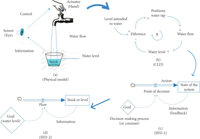
In Fig. 2 the process of building a model is shown in a simple example: filling of water reservoir, until a desired limit. To model this system, one starts from a physical model (Fig. 2a), translates it to a CLD (Fig. 2b), subsequently making a SFD (Fig. 2c), then eventually refining it in a second SFD (Fig. 2d). From this point, the mathematical equations that describe the system can be formulated (Sterman 2000; Forrester 2009).
In this work the commercial software VENSIN® was used to build the CLDs and SFDs, and simulate the system.
Figure 2. Example of modeling process with system dynamics. Adapted from Forrester (2009),
Sterman (2000) and Asif et al. (2015).
Level intended to water Actuator
(Hand)
Control
Information Sensor
(Eye)
+
+
+ +
–
Water level Water level
Stock (b)
(CLD)
(c) (SFD-1)
Information (Feedback)
State of the system Point of decision
Action
Goal
Decision-making process (or constant)
(d) (SFD-2)
Information Stock or level Flow
Goal (water level)
(a) (Physical model)
B
Diference Water flow
Water flow
Positions water tap
METHODOLOGY
THE STH/SD METHODOLOGY
This section describes a process for combining stakeholder theory with systems dynamics methodology into a new methodology, the STH/SD methodology, which is used to model and simulate PEB’s dynamics. In this new methodology,
first the main stakeholders are identified and classified following Mitchell et al. (1997) categories. The classification and
identification of the most relevant STHs of the system as suggested by Mitchell et al. 1997 is on the basis of the proposed
over time. This dynamics of STHs led to the possibility of associating the STH theory with the SD methodology. Another important consideration is that, if it were not for the synthesis, which the classification and identification of STHs allows, it would be much more difficult to produce models that can be simple, lean, simulated and representative of the dynamics of the system. The practical and very important result to be achieved by this STHs identification and classification is the possibility to capture, from a complex system, a sample, the most representative of its main STHs. This sample of STHs will be used to design a simplified first version of the dynamic model of the system. Then, the STHs objectives and activities (concern and expectations) are listed in a table, such that possible parameters (elements) for the construction of the dynamic model can be identified. Casual Loop Diagrams (CLD) and Stock and Flow Diagrams (SFD) are then built based on the elements identified.
The elements of SD modeling (stocks, flows and variables) act as sensors and actuators within the network of STHs. These sensors are responsible for capturing STH status variations. Assuming that STH behavior is dynamic, changes over time, the STH and SD modeling process must (1) be able to capture the most relevant STHs of the system (to enable a simplified model to be built) and (2) allow monitoring STH behavior through the analysis of their sensors and actuators (stocks, flows and variables). Through the simulation of the dynamic behavior of this system (e.g. PEB), it can be inferred how to act in the system to correct possible disturbances.
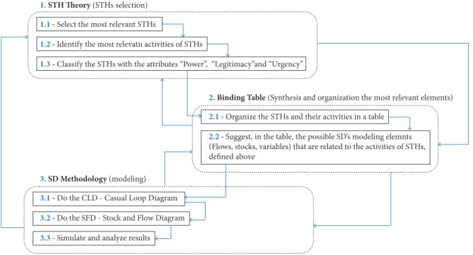
The whole process is shown in the workflow of Fig. 3. Note that the workflow suggests that the process is recursive. That is, during the steps of stakeholder identification and CLD and SFD design, it should always feedback the table (binding table) to ensure that it will be the most simple and representative as possible of the system being studied.
As is shown in Fig. 3, the workflow is composed of three main steps:
• Step 1: Make the selection of the most relevant stakeholders and assign to each of them one or more of the attributes
power, legitimacy and urgency.
• Step 2: Arrange the STHs in a table and list their most relevant activities to the system; propose, to each activity
listed, a possible variable or flow or stock (i.e. elements of SD modeling) that best represent them. This table (binding table) is responsible for linking STH theory and SD methodology. STH activities will be interpreted as stakes. Stakes
Figure 3. STH/SD Workflow combining STH Theory and SD Methodology. 1. STH Theory (STHs selection)
1.1 - Select the most relevant STHs
1.2 - Identify the most relevatn activities of STHs
1.3 - Classify the STHs with the attributes “Power”, “Legitimacy”and “Urgency”
3. SD Methodology (modeling)
3.1 - Do the CLD - Casual Loop Diagram
3.2 - Do the SFD - Stock and Flow Diagram
3.3 - Simulate and analyze results
2. Binding Table (Synthesis and organization the most relevant elements)
2.1 - Organize the STHs and their activities in a table
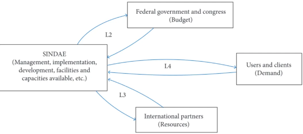
Figure 4. Representation of main actors of SINDAE.
will be translated as potential elements of SD modeling (variables, flows and stocks) that will allow the construction of the Causal Loop Diagram (CLD) and later the Stock and Flow Diagram (SFD).
• Step 3: Design the CLD and SFD; simulate the evolution of the system given initial conditions and analyze the results.
With those three steps completed, it can be checked recursively if step-1 needs to be adjusted and therefore step-2. Once
completed the first SFD, the system model is built using the software VENSIM® and simulations performed. Here we are
firstly interested in finding a stable model. Hence, if the simulation results show an unstable system, its architecture and/ or variables are modified until that is achieved.
To start the process of modeling, it should also be outlined the STH’s network that make up the system. It should give an initial idea of what are the most relevant STHs in the system and how they are connected.
CASE STUDY
The beginning of the Brazilian space program dates back to the 1960s, with the creation of the Organizing Group of the National Commission on Space Activities (GOCNAE). In its first years PEB was focused on implanting basic laboratory infrastructure and formation of human resources (HR), mainly on space science, early Earth applications of space technology in remote sensing and telecommunications, and sub-orbital rockets.
In the late 1960s and early 1970s were created the Space Activities Institute (today the Aeronautics and Space Institute – IAE) and the Space Research Institute (today National Institute for Space Research – INPE). The former one, subordinated to the Brazilian Air Force, was responsible for rocket research and development, while INPE, then subordinated to the civilian National Research Council (now National Council for Scientific and Technological Development – CNPq), replaced GOCNAE on its research and development activities. GOCNAE was extinct in 1971.
In the late 1970s, PEB received a great push with the establishment of the Brazilian Complete Space Mission (MECB), which had the strategic objective of enabling the country to develop launchers and satellites on its own. The first goals of MECB were to put in orbit four small satellites, using Brazilian rockets, from a Brazilian launch site. Though not fully realized, MECB laid the grounds of much of the infrastructure (both physical and human resources) related to access and use of space existing today in Brazil.
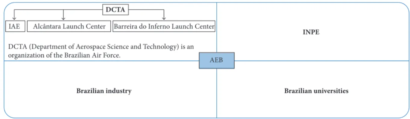
PEB’s current structure was established in the mid-1990s with the creation of the Brazilian Space Agency (AEB), responsible to formulate and revise periodically the National Program for Space Activities (PNAE) (AEB 2012). At that time an update of the National Policy for the Development of Space Activities (PNDAE) (Brasil 1994) was released and established the National System for the Development of Space Activities (SINDAE) (Brasil 1996). The main purpose of SINDAE is to organize the execution of activities aimed at national space development. Under the central coordination of AEB, SINDAE embodies other organizations, governmental and private, which are responsible for execution of PNAE actions and programs. In Fig. 4 is shown a representation of SINDAE, depicting its main present actors (stakeholders).
INPE DCTA
IAE Alcântara Launch Center Barreira do Inferno Launch Center
DCTA (Department of Aerospace Science and Technology) is an organization of the Brazilian Air Force.
Brazilian universities Brazilian industry
The development and expansion of the Brazilian Space Program rely on national partnerships established with ministries, departments and other governmental agencies that may finance part of the national interest projects. International partnerships have also been used as a way to share the high costs and risks associated with satellite development. There are within the Brazilian government various units which are users, even potential ones, of space systems, and that can be financial agents of PNAE’s activities implementation.
Considering only the public sector financial resources (AEB 2017), the projects related to PEB turnover were of approximately $200 million dollars per year between 2011 and 2015. This budget was applied in specific activities like R&D and services related to satellites and their applications, launch vehicles, ground infrastructure, workforce training and management. Considering the private sector, according to the Brazilian Aerospace Industries Association (AIAB 2016), there are currently approximately 50 industries, which generate approximately 25,000 direct jobs, working in the Brazilian aerospace industry, all of which are able to provide services to answer the PEB’s projects demands. However, the revenue from strictly space activities represented in 2013 approximately $24.8 million dollars (0.46% from total). In 2015 the revenue, with space activities, was reduced to $5.16 million dollars, which represented 0.089% from total.
Despite important results achieved by PEB, there are indicators that point to a scenario of stagnation and decline of space activities in the country. In addition to the decrease in revenue mentioned in the previous paragraph, there is a worrying reduction of PEB’s workforce and investment in new projects, which are already impacting on the technical capacity of its main executors (Cardoso 2012; AEB 2012; AAB 2010; Bartels 2016). On the other hand, initiatives such as the Strategic Program of Space Systems (PESE) (Camilo 2016), and the already huge demand existing in Brazil for space services and products, most of it now fulfilled by foreign space systems, highlights the potential for a robust increment of PEB activities in the future.
Modeling PEB with system dynamics can help on understanding that contradiction, while providing its managers a tool for simulating the Program’s possible future scenarios, and then helping on the strategic planning of a long term sustainable Program.
Following the process shown in Fig. 3, are first identified the most relevant STHs for the system (PEB), following
the approach of STH classification suggested by Mitchell et al. (1997). It’s important to notice that the PEB’s model
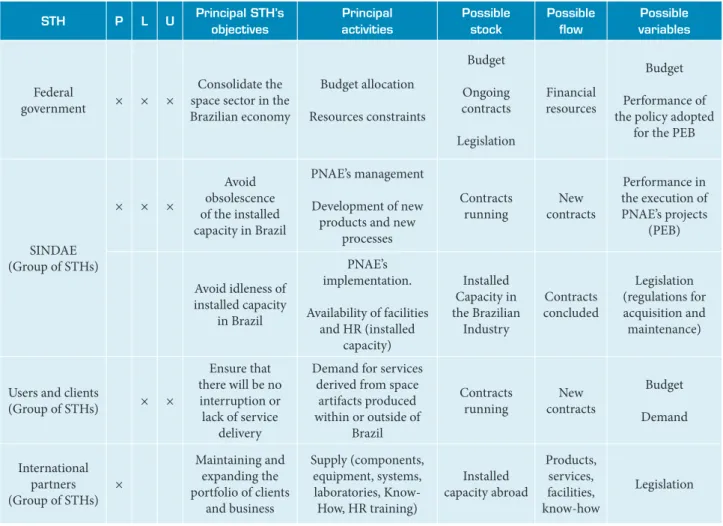
will be a simplified representation of the real system. The identification and classification of STH, with at least one of the three attributes, will help in the process of building a simple but representative model of the system. For this study we considered only four main stakeholders: SINDAE, the Federal Government, international partners and the users (even potential ones) of PEB’s products and services. Note that these stakeholders represent in fact groups of stakeholders, but we think that, for the purposes and depth of the present study, they represent the nodes of the system to be modeled, in terms of planning, provision of resources, demands and execution. These stakeholders were then classified with at least one of the attributes power (P), legitimacy (L) and urgency (U), see in Table 1 columns (P), (L) and (U).
Table 1. STH/SD Table (the binding table). STHs classification and suggestion of SD elements to compose the CLD and SFD.
STH P L U Principal STH’s
objectives Principal activities Possible stock Possible flow Possible variables Federal
government × × ×
Consolidate the space sector in the Brazilian economy Budget allocation Resources constraints Budget Ongoing contracts Legislation Financial resources Budget Performance of the policy adopted
for the PEB
SINDAE (Group of STHs)
× × ×
Avoid obsolescence of the installed capacity in Brazil
PNAE’s management
Development of new products and new
processes Contracts running New contracts Performance in the execution of PNAE’s projects
(PEB)
Avoid idleness of installed capacity
in Brazil
PNAE’s implementation.
Availability of facilities and HR (installed
capacity) Installed Capacity in the Brazilian Industry Contracts concluded Legislation (regulations for acquisition and maintenance)
Users and clients
(Group of STHs) × ×
Ensure that there will be no
interruption or lack of service
delivery
Demand for services derived from space
artifacts produced within or outside of
Brazil Contracts running New contracts Budget Demand International partners (Group of STHs)
×
Maintaining and expanding the portfolio of clients
and business
Supply (components, equipment, systems, laboratories,
Know-How, HR training)
Installed capacity abroad Products, services, facilities, know-how Legislation
P = attribute Power; L = attribute Legitimacy; U = attribute Urgency.
Then, based on Table 1, a first CLD was devised to represent the system, as shown in Fig. 5.
In the CLD-1, Loop-1 (L1) represents the exchange of information regarding demands, generated by PEB’s users. Loop-2 (L2) represents mainly the exchange of budget, provided by the Brazilian federal government, and products and services delivered by SINDAE in response to that funding. Loop-3 (L3) represents mainly the international partners capacity to support the PEB’s implementation. Are included in this context the international suppliers of components, equipment, systems, laboratories and know-how, and educational and research institutes which contribute, for example, for educating and training Brazilian experts. Loop-4 (L4) shows mainly the implementation activity of PEB, and can be represented by results achieved & results expected, i.e., the performance in the PEB’s projects implementation. Loop-5 (L5) represents mainly the other demands that are not met through the SINDAE.
It can be said that the main interactions between PEBs stakeholders occur through SINDAE. Hence, for this preliminary work, Loops 1 and 5, in Fig. 5, will not be considered in the PEBs modeling. Adding to the CLD-1 the major activities of STHs and removing from it Loops 1 and 5, it is constructed CLD-2, depicted in Fig. 6.
Using again the recursive workflow (Fig. 3) and analyzing CLD-2 and Table 1, it can be constructed a new CLD (CLD-3), shown in Fig. 7, where the variables and exchange of resources in the system are represented instead of the stakeholders.
Figure 5. Causal Loop Diagram 1 (CLD-1), representing the paths of resources exchange between groups of PEB’s stakeholders.
Figure 6. Causal Loop Diagram 2 (CLD-2), representing the paths of resources exchange between groups of PEB’s stakeholders.
Figure 7. Causal Loop Diagram (CLD-3), for a (Simplified PEB’s market model). Based on the fundamental models of dynamic behavior (Sterman 2000).
Federal government
SINDAE
International partners
Users L4
L2
L3
L1
L5
L4 L2
L3
Federal government and congress (Budget)
SINDAE
(Management, implementation, development, facilities and
capacities available, etc.)
Users and clients (Demand)
International partners (Resources)
Demand Discrepancy
Suppliers
Budget
-+ +
+ +
B1
B2 Goal for
Contract in Progress
+
+
It can be said that CLD-3 has two balanced loops, B1 and B2. In loop B1 it is represented the balance between the numbers of contracts (projects) put in industry, necessary to sustain a planned industrial policy, and the capacity of the industry in fulfilling this goal. This balance is assessed through the discrepancy parameter. Note that the discrepancy may be a measure of performance expected for the system. In Loop B1 are represented only companies that are contracted directly by the Brazilian government, the main contractors. Loop B2 represents the supply chain, composed by national and international companies that could provide support for the contracts in progress. An increase in the value of discrepancy requires, or induces, an increase in the supply chain, which potentially allows an increase in the contracts in progress. Note also that there is a time delay component that should have been considered in this CLD; however, to simplify the modeling, the delay was not modeled.
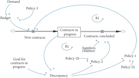
The demand, reported in Table 1 and represented in CLD-3, is an element that triggers the available budget both during the planning and the implementation of projects (in this representation, the demand increase always creates a budget increase). One possible way of representing Loops B1 and B2, from Fig. 7, as a SFD is seen in Fig. 8.
Figure 9. SFD-2 (Rearrangement of SFD-1).
Figure 8. SFD-1. Loops B1 and B2 from CLD-3 represented as a Stock and Flow Diagram (SFD).
Policy-2 Contracts in
progress
New contracts Contracts concluded
Suppliers (Market) +
Discrepancy
-Goal for contracts in
progress
+
+
Policy-1 B2
B1 Budget
+ +
-
+Demand
+
Policy-3
+
Policy-2S +
Policy-1S + +
-Goal for contracts in progress +
+ +
B1
B2 Suppliers (Market)
Budget-1 Demand
Discrepancy
New contracts Contracts concluded Contracts
in progress
The mathematical meaning of each element in SFD-2 is described below:
Discrepancy (Variable)
This is a variable to measure the disagreement between the stock of contracts in progress and the goal desired to it. Discrepancy is used to monitor the stock level Contracts in Progress by comparing it to a desired value Goal for Contracts in Progress. If the stock does not correspond to the desired value, the system reacts to this difference, acting on the input and output flows, to rebalance the stock. When the system is balanced the value of this variable is one.
In this first model, what is wanted to analyze and control is the (feasible) level of contracts that the PEB must impose on the Brazilian and international supplier market. An excess of demand directed to the (still immature) Brazilian supplier market can overwhelm the Brazilian industries lead simply to an increase of imported goods, instead of a stimulus to an increase of Brazilian space industry capacity. In this context, the variable discrepancy must act simultaneously in the flows input and output of the stock contracts in progress, which will allow the analyst to find a good relation between the flows New Contracts and Contracts Concluded ensuring that there is an incremental growth of the Brazilian supply chain. Discrepancy will be configured to be greater than one if the Goal for Contracts in Progress is higher than the stock Contracts in Progress (Eq. 1):
Discrepancy = Goal for Contracts in Progress / Contracts in Progress
where the unit is dimensionless.
Policy-1and Policy-2 (Auxiliary Variables)
Variables Policy-1 and Policy-2 represent the government policy desired to influence, respectively, the flow of New Contracts and Contracts Concluded and so control the level of stock Contracts in Progress. They are based in the discrepancy observed between contracts in progress and the goal desired to contracts in progress. Policy-1 represents the government’s financial incentive policy for new contracts to be admitted or rejected in the system. It relates the number of contracts with financial resources. Policy-2 represents the government’s incentive policy to the contracts to be completed, delayed or accelerated each year. It relates completed contracts with the unit of time. When the system is stable, the variable Discrepancy is equal to one. In this model it is assumed that if discrepancy is less than one, the flow contracts concluded is increased and the flow new contracts is reduced to restore the stock’s level contracts in progress. On the other hand, if the variable discrepancy is greater than one, the flow of contracts concluded is reduced and the flow of new contract is increased. In this way, Policy-1 is directly proportional to Discrepancy and Policy-2 is inversely proportional. Other two variables were created to support Policy-1 and Policy-2. They are nominated as Policy-1S and Policy-2S. Their objective is (1) to allow adjusting the values of the model units and (2) to study how the system reacts by increasing and/or decreasing Policies-1 and 2 (Eqs. 2 to 5):
Policy-1 = Policy-1S × Discrepancy
Policy-1S = 1
where the units are contracts/R$.
Policy-2 = Policy-2S × (1 / Discrepancy)
Policy-2S = 1
where the units are contracts/year.
(1)
(5) (4) (2)
Policy-3 (Auxiliary Variables)
Policy-3 is related to the budget allocated to each project. It is noteworthy that the execution of a project may require that one or more contracts be implemented (Eq. 6).
Policy-3 = 1 where the unit is R$/project.
Contracts in Progress (Stock)
Represents the stock of contracts existing at a given time. This stock is a function of the number of new contracts signed and the number of contracts concluded each year. It is important to notice that this stock may reflect the government’s strategy of promoting the industry. The Brazilian Government has been implementing an industrial policy in order to ensure the survival, and aimed at the grown and consolidation of the space sector in the Brazilian economy (Oliveira 2014; AEB 2012; Schmidt 2011;
Dewes et al. 2010; 2015) (Eq. 7).
Contracts in Progress = Number of contracts at time t
0 +
∫
t t 0
(New contracts – Contracts concluded)
where the current value in time t
0 = 10 contracts; and the unit is contracts.
Supplier Market (Variables)
Represents a stock of resources (human and material) installed and available (in Brazil and abroad) to support the PEB’s projects implementation (supply chain). For this exercise the supplier market will be represented by a variable that does not interfere negatively with the projects implementation, i.e., the supplier market has 100% availability to meet the PEB (considering time, cost and quality) (Eq. 8).
Supplier Market = 1 where the unit is dimensionless.
Contracts Concluded (Flow)
Represents the flow of contracts finished per year. This flow is a function of the installed capacity in the supplier market and of the government policy assigned to PEB (Policy-2) (Eq. 9).
Contracts Concluded = Policy-2 × Suppliers (Market)
where the unit is contract/year.
Demand (Variable)
It represents, for example, the demand of Brazilian users/clients (civil, defense and government) for space missions, to be executed by PEB. For this exercise, we adopted a hypothetical demand of 1 project (this value can be changed during the simulation to see the system’s response). Note that in the real world a single demand may produce several contracts (Eq. 10).
Demand = 1
where the unit is projects/year.
(8) (7) (6)
(9)
Budget (Variable)
It is a variable that represents the governmental budget availability to PEB implementation. It could be a function of demand and/ or expected results, in this way, an increase in demand or expected performance would imply in an increase in budget availability. Note that this is a hypothetical assumption, since, for example, in the real world an increase in demand may not necessarily result in an increase of available budget. So, for this first approach the budget is the variable that relates “Demand” and “Policy-3” and will be dimensioned as (Eq. 11):
Budget = Demand × Policy-3
where the unit is R$/year.
New Contracts (Flow)
Represents the flow of new contracts signed each year. This flow can be represented, for example, by the historical average number of contracts signed each year in PEB or by the policy for new contracts that the government strategically determines for this sector. Or, new contracts can be represented by an independent variable whose goal would be to regulate the maintenance or increase of the stock of contracts in progress. For this first exercise it was decided to make this flow equal to (Eq. 12):
New Contracts = Policy-1 × Budget
where the unit is contract/year.
Goal for Contracts in Progress (Variable)
It is a variable that represents a desired performance to PEB, from the government point of view to consolidating the Brazilian space industry. Considering that one of the strategic guidelines of PEB is to “Consolidate the Brazilian space industry, by increasing its competitiveness and innovation capacity, also through the use of the State’s purchasing power and the partnerships with other countries” (AEB 2012), the number of government contracts in progress may be used as one of the performance parameters of PEB. It was considered that the government’s policy is to maintain a hypothetical stock of N contracts in progress, in order to ensure the maintenance and progression of PEB and of the Brazilian industrial space sector. For this exercise was adopted N = 10 (Eq. 13).
Goal for Contracts in Progress = 10
where the unit is contracts.
RESULTS AND DISCUSSION
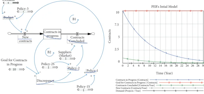
SFD-2 SIMULATION RESULTS
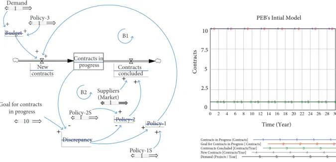
A model for the system was built using software VENSIM®. A simulation considering the boundary conditions described
above was performed and the results are shown in Fig. 10. In Fig. 10a, the SFD-2 is represented in VENSIN® using scales for the
variables: Demand, Policy-3, Policy-1S, Policy-2S, goal for contracts in progress, and Suppliers (Market).
It is important to note that the time scale observed in Fig. 10b refers to an exploratory study of possible ways to model PEB and may not correspond (in this initial study) to the time scales observed in more realistic simulations to be done in the future. It is a simulation with hypothetical data with the objective of gaining expertise in the modeling of PEB.
So, using the model of Fig. 10a, the first simulation test (Test-1) was done (see Fig. 10b). In Test-1, it was considered that the stock level contracts in progress equals 10 contracts (see Fig. 10b, curve 1, blue) and its goal for contracts in progress is also (11)
(12)
equal to 10 contracts (curve 2, red). In this condition the input flow New Contracts (curve 4, gray) and the output flow Contracts
Concluded (curve 3, green) are equal to 1 and the system remains stable (from time t0 until the end of the simulation). Note that
the input flow depends on Policy-1 and the output flow depends on Policy-2. Policy-1 is directly proportional to the discrepancy variable and Policy-2 is inversely proportional to it.
Figure 10. SFD-2 simulation results (Test1 – stabilized system).
Policy-2 Contracts in
progress New
contracts Contractsconcluded
Suppliers (Market)
+
Discrepancy
-Goal for contracts in progress
+
+
Policy-1 B2
B1 Demand
+
Budget
-
+Policy-2S +
Policy-1S
+
Policy-3
+ +
+
1
10 1
1
1
1 PEB's Intial Model
10
7.5
5
2.5
0
5 5 5 5 5 5 5
4 4 4 4 4 4 4
3 3 3 3 3 3 3 3
2 2 2 2 2 2 2 2
1 1 1 1 1 1 1 1
0 2 4 6 8 10 12 14 16 18 20 22 24 26 28 30
Time (Year)
C
on
tracts
Contracts in Progress (Contracts] 1 1 1 1 1
Goal for Contracts in Progress [ Contracts] 2 2 2 2
Controacts Concluded [Contracts/Year] 3 3 3 3 3
New Contracts [Contracts/Year] 4 4 4 4 4
Demand (Projects / Year] 5 5 5 5 5
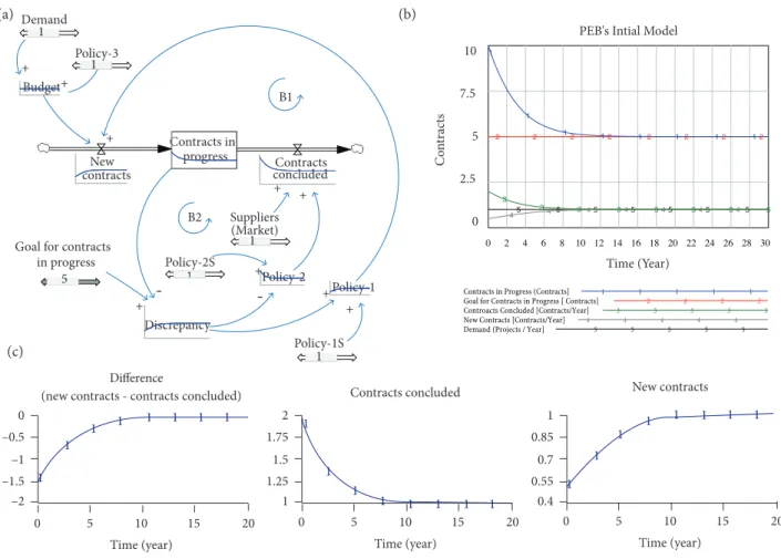
In a second simulation, a change was imposed to the system removing it from the stability condition, as shown in Fig. 11a. In Test-2, the goal for contracts in progress was set to 5 contracts. This means that in an instant of time the stock and its goal were in
equilibrium (equal to 10 contracts) and, in the next time instant (in t0+n), this balance was broken, because the stock remained equal
to 10 while its objective was suddenly changed to 5 contracts. This causes the value of Policy-1 to go from 1 to 0.5 (instantaneously closing the input flow new contracts) and the value of Policy-2 changes from 1 to 2 (instantly opening the output flow contracts concluded). This is the operation logic that will cause the model to begin the process of reducing the stock level.
The diagram of Fig. 11b (curve 1, blue) shows the stock level of contracts in progress converging to the goal (curve 2, red). The graphics of Fig. 11c show details of the input and output flows, respectively new contracts and contracts concluded, which fill and drain the stock.
Looking the Fig. 11c it is noticed that, in the beginning of simulation, there is a large difference between the input flow (equal to 0.5) and the output flow (equal to 2), respectively New Contracts and Contracts Concluded. It is expected, however, that the system react to this abrupt initial difference, between the two flows, gradually stabilizing the stock to avoid the complete emptying of the stock. The balanced loops, set by Policies 1 and 2, influence the shapes of the response flow curves, shown in Fig. 11c. The dynamics of the system gradually compensate the initial closing of the input flow, opening it gradually, and in the same way compensating the initial opening of the output flow, also closing it gradually. Note that the difference between the input flow and the output flow decreases over time, causing the system to stabilize.
In Test-3 another possible change is simulated. For example, suppose that the system is stable with the stock contracts in progress and its goal equal to 10 (like in the Test-1) and that, suddenly, the input flow new contracts is stopped. Note that, if the system represents the PEB, this change could mean that the demand or/and Budget would be reduce to zero.
The answer for this change, in the PEB’s hypothetical model, is shown in Fig. 12, that is, the stock of contracts in progress would be reduced by approximately 50% (5 contracts) over a period of 7 years (Fig. 12b, curve 1, blue) and reduced to zero after approximately 30 years. Note that this result reflects hypothetical, nonrealistic, values for the system elements (variables, flows and stocks). However, this partial and simplified model of PEB shows the potential of systems dynamic modeling, as a tool for predicting possible future scenarios for the Program.
Another scenario (Test-4) that could be simulated using SFD-2 would be: What could happen to the system if we imposed on it 2 changes simultaneously?, for example, (1) Increase the Goal for Contracts in Progress by 100%, changing it to 20 (contracts) and; (2) simultaneously, increase the demand for new projects by 100%, changing it to 2 projects/year. In Fig. 13a, it is shown what happens with the system.
Note that the stock converges to 28 contracts in progress, 8 contracts above the goal set for it. This means that the Policy-1 and Policy-2 were not robust enough to compensate the system for the change in the variables.
A possible solution to adjust the system is to increase the output flow Contracts concluded. This can only be done by changing Supplier Market and/or Policy-2. As Supplier Market has already been scaled as 100%, we have as an alternative only to adjust the variable Policy-2. This was done by changing Policy-2, in a way that the flow contracts concluded also increases proportionally to demand, in such a way that it compensates the increase in the flow new contracts. In SFD-2, the Policy-2 equation was changed to (Eq. 14):
Policy-2 = Policy-2S × Demand × (1 / Discrepancy)
Figure 11. Test-2 (a) SFD-2 (Goal for Contracts in Progress is set to 5); (b) SFD2 – Simulation response to goal = 5 contracts; (c) SFD-2 – Flows IN/OUT difference.
Policy-2 Contracts in
progress New
contracts concludedContracts
Suppliers (Market) +
Discrepancy
-Goal for contractsin progress + + Policy-1 B2 B1 Demand + Budget
-
+ Policy-2S + Policy-1S + Policy-3 + + 1 5 1 1 1 1PEB's Intial Model 10
7.5
5
2.5
0
5 5 5 5 5 5 5
4 4 4 4 4 4 4
3
3 3 3 3 3 3 3
2 2 2 2 2 2 2 2
1
1
1 1
1 1 1 1
0 2 4 6 8 10 12 14 16 18 20 22 24 26 28 30
Time (Year)
Contracts in Progress (Contracts] 1 1 1 1 1
Goal for Contracts in Progress [ Contracts] 2 2 2 2
Controacts Concluded [Contracts/Year] 3 3 3 3 3
New Contracts [Contracts/Year] 4 4 4 4 4
Demand (Projects / Year] 5 5 5 5 5
C on trac ts 1 1 1 1 1
1 1 1 1
1 1
1 1
1 1 1 1
1
1 1 1 1 1 1
0 –0.5 –1 –1.5 –2
(new contracts - contracts concluded) 2 1.75 1.5 1.25 1 Contracts concluded 1 0.85 0.7
0 5 10 15 20
0.55 0.4
New contracts
Time (year)
0 5 10 15 20
Time (year)
0 5 10 15 20
Time (year)
Difference
(a) (b)
(c)
Figure 12. Test-3 – SFD-2, simulation results to Demand equal zero.
Now the system stabilizes at the targeted stock, as seen in Fig. 13b (curve 1, blue). Note that the consideration that Policy-2 is directly proportional to demand, as put in Eq. 14, is somehow arbitrary, meaning here only that the flow new contracts must be opened as a function of demand.
In the tests made so far, the supplier market was dimensioned as having 100% capacity. In the real world it may be considered (at the beginning of a mission) that a given supply chain will be necessary and sufficient to meet a given project, however, with the progress of the project it would be necessary to extend or modify the initially proposed supply chain (due to technological, legal, financial, etc., restrictions). Moreover, the supply chain is composed of Brazilian and international industry that have different sizes and capacities. The Brazilian space industry is small and is being structured. On the other hand, there is already a structured and efficient supply chain (i.e. structured and mature market segment) in countries whose space programs are more developed than PEB, for example, China, Russia, European Union and USA.
C on trac ts Policy-2 Contracts in progress New
contracts ConcludedContracts
Suppliers (Market) +
Discrepancy -Goal for Contracts
in Progress + Policy-1 B2 B1 Demand + Budget - + Policy-2S + Policy-1S + Policy-3 + + + 1 10 0 1 1 1
PEB's Intial Model 10
7.5
5
2.5
0 45 45 45 45 45 45 45 3
3 3
3 3 3 3 3
2 2 2 2 2 2 2 2
1 1 1 1 1 1 1 1 0 2 4 6 8 10 12 14 16 18 20 22 24 26 28 30
Time (Year)
Contracts in Progress (Contracts] 1 1 1 1 1 Goal for Contracts in Progress [ Contracts] 2 2 2 2
Controacts Concluded [Contracts/Year] 3 3 3 3 3 New Contracts [Contracts/Year] 4 4 4 4 4
Demand (Projects / Year] 5 5 5 5 5
Figure 13. Test-4, SFD-2 simulation results with (a) 100% Demand and Goal increase; (b) 100% Policy-2 increase. PEB's Intial Model
30
22.5
15
7.5
0 45 45 45 45 45 45 45
3 3 3 3 3 3 3
2 2 2 2 2 2 2 2
1 1 1 1 1 1 1 1
0 2 4 6 8 10 12 14 16 18 20 22 24 26 28 30
Time (Year)
Contracts Contracts
Contracts in Progress (Contracts] 1 1 1 1 1
Goal for Contracts in Progress [ Contracts] 2 2 2 2
Controacts Concluded [Contracts/Year] 3 3 3 3 3
New Contracts [Contracts/Year] 4 4 4 4 4
Demand (Projects / Year] 5 5 5 5 5
PEB's Intial Model 20
15
10
5
0
5 5 5 5 5 5 5
4
4 4 4 4 4 4
3 3 3 3 3 3 3 3
2 2 2 2 2 2 2 2
1 1
1
1 1 1 1 1
0 2 4 6 8 10 12 14 16 18 20 22 24 26 28 30
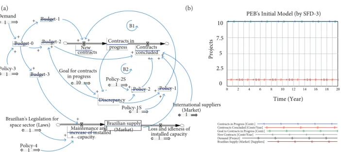
SFD-3 SIMULATION RESULTS
From the results and observations made above, it is clear that SFD-2 should be modified to better represent the system. As an example of a possible improvement for SFD-2, taking into account the discussions made above, the stock and flow diagram are shown in Fig. 14 (SFD-3).
In SFD-3, the following main modifications were done:
1. The supply chain was divided into two, one representing the Brazilian industry, the other the international industry. This
make possible to include in the model other elements presented in Table-1, translated in SFD-3 as Brazilian Legislation for Space Sector, Maintenance and Increase of Installed Capacity, Loss and Idleness of Installed Capacity and the Policy-4, all of them related to the Brazilian industry.
2. The Budget variable is divided into 3 parts: i) one that acts over the input flow New Contracts – Budget-1; ii) other that
acts over the output flow Contracts Concluded – Budget-2, and a third; iii) that acts over the contracts that goes to the Brazilian supply industry - Budget-3. Note that the budget could still be fragmented into more parts and the Policy-3 could follow it. However, we are gradually adding complexity to the system.
3. As learned during the previous test (Test-4) the variable Demand must be modeled to influence (even indirectly) the
input flow New Contracts and output flow Contracts Concluded. This is implemented, causing the demand variable to be associated with Budget-1, to influence the input flow, and associated with Budget-2, to influence the output flow. Note that we are gradually adding complexity to the system and for this particular model we are assuming that an increase in demand implies an increase in budget which, in the real world, may not occur.
The new elements representing SFD 3 are defined as follows:
Budget-0, 1, 2 and 3 (Variables)
The principal Budget (Budget-0) was divided in to three equal parts (Eqs. 15 and 16).
Budget-0 = 1
Budget-1 = Budget-2 = Budget-3 = (Budget-0)/3
where the unit is R$/year.
Figure 14. (a) SFD-3 and (b) simulation results considering the system stable. Policy-2
Contracts in progress New
contracts concludedContracts
International suppliers (Market) +
Discrepancy -Goal for contracts
in progress
+
+ Policy-1
B2 B1
Budget-0 Budget-2 +
+ Budget-1 - + + + + Brazilian supply (Market) Maintenance and
increase of installed capacity
Loss and idleness of installed capacity
+
Brazilian's Legislation for space sector (Laws)
+ Budget-3 + + + Policy-3 Demand + + Policy-4 + Policy-1S + Policy-2S + 1 10 1 1 1 1 1 1 1
PEB's Initial Model (by SFD-3) 10
7.5
5
2.5
0 456 456 456 456 456 456 4
3 3 3 3 3 3 3
2 2 2 2 2 2 2
1 1 1 1 1 1 1
0 2 4 6 8 10 12 14 16 18 20
Time (Year)
P
ro
jec
ts
Contracts in Progress [Contr.] 1 1 1 1 1
Controacts Concluded [Contr/Year] 2 2 2 2 2
Goal to Contracts in Progress [Contr] 3 3 3 3 3
New Contracts [Contr/Year] 4 4 4 4
Demand [Project] 5 5 5 5 5
Brazilian Supply (Market) [Suppliers] 6 6 6 6
(15)
(16)
Policy-2, Policy-2S and Policy-3 (Auxiliary Variables)
Variables Policy-2 and 2S represent the relation between contracts, financial resources and number of suppliers involved each year with the flow of contracts conclude. Policy-3 maintained the same definition as in SFD-2, however, its value was modified to adjust the equal distribution of budgets (Budget-0) (Eqs. 17 to 19).
Policy-2 = Policy-2S × (1 / Discrepancy)
Policy-2S = 1
where the unit is [(contracts/year) / (R$/year)] / suppliers.
Policy-3 = 3
where the unit is R$/project.
Policy-4 (Auxiliary Variable)
The Variable Policy-4 represents the relation between suppliers and financial resources involved with the flow of Maintenance and Increase of Installed Capacity (Eq. 20).
Policy-4 = 1 where the unit is suppliers/R$.
International Suppliers (Market), (Variable)
Represents a stock of resources (human and material) installed and available, abroad, to support the PEB’s projects implementation (supply chain). For this exercise the International Suppliers (Market) will be represented by a variable that does not interfere negatively with the projects implementation, i.e., it has 100% availability to meet the PEB (considering time, cost, quality and the law) (Eq. 21).
International Suppliers (Market) = 1
where the unit is dimensionless.
Brazilian’s Legislation for Space Sector (Laws), (Variable)
Represents the Brazilian legislation that supports the PEB’s projects implementation. For this exercise the Brazilian Legislation for Space Sector (Laws) will be represented by a variable that does not interfere negatively or positively with the projects implementation (Eq. 22).
Brazilian’s Legislation for Space Sector (Laws) = 1
where the unit is dimensionless.
Brazilian Suppliers Market (Stock)
Represents a stock of resources (human and material) installed and available in Brazilian market to support the PEB’s projects implementation (supply chain). It represents the infrastructure (laboratories, specialized human resources, etc.) contained in all STHs (public and private) that make up SINDAE. This technological patrimony is the core of the Brazilian space sector and (17)
(18)
(19)
(20)
(21)
consequently one of the main elements for the construction, consolidation and sustainability of the Brazilian industrial policy for the space sector (Eq. 23).
Brazilian Suppliers (Market) = Number of Brazilian Suppliers at time t
0 +
+
∫
tt 0
(Maintenance and increase of installed capacity – Loss and idleness of installed capacity)
where the current value in time t
0 = 1 Supply; and the unit is suppliers.
Maintenance and Increase of Installed Capacity (input Flow)
Represents the flow that fills the stock Brazilian Suppliers (Market). The control of this flow is related to the Brazilian policy that should be used to (1) maintain in good condition, (2) expand, and (3) improve the PEB’s facilities (Eq. 24).
Maintenance and Increase of Installed Capacity = = Budget-3 × Brazilian’s Legislation for Space Sector (Laws) × Policy-4
where the unit is suppliers/year.
Loss and Idleness of Installed Capacity (output Flow)
This flow represents the flow that drains the stock Brazilian Suppliers Market. This drain could be caused, for example, by the deterioration of the infrastructure and equipment of the laboratories or by the idleness of the resources (human and material) that compose them. Potentially, these factors, combined or isolated, can make the Brazilian supply chain (which is in the process of formation) obsolete or, in the last analysis, can promote its deterioration due to lack of maintenance and recycling. It can be said then that the loss and idleness of this installed capacity degrades the suppliers HR and the facilities, disqualifying them for the PEB’s activities (Eq. 25).
Loss and Idleness of Installed Capacity = 1
where the unit is suppliers/year
Considering that the system shown in Fig. 14 (SFD-3) is initially stabilized, its behavior can be simulated for a new scenario (Test-5). The new scenario would allow the following questions to be answered: What would happen to the System if demand for new projects increased, for example, by 15%? What elements of the system could be adjusted to compensate for that increase? The graph of Fig. 15a shows the behavior of the system considering a demand increase of 15%. Note that this increase had a positive impact on 3 elements of the system: the flow of New Contracts, the flow of Contracts Concluded and the stock of Brazilian Supply Market, however, the increase of these elements directly influence the input and output flows of the Contracts in Progress stock, reducing its level from 10 to 5 contacts over a period of 5 years. One of the possible conclusions for this behavior is that there is a difference between the growth of the inflows and outflows of the stock Contracts in Progress (see graphs of Fig.15a, respectively, curves 4, grey and 2, red). One of the possible solutions to correct that difference and consequently to correct the stock level Contracts in Progress would be to review the distribution of budgets (which directly influence the input and output flows) and also to review the target set for the level of the contracts stock Goal for Contracts in Progress. The graphs of Fig. 15b show the behavior of the system considering an increase in the Budget-1 of 100% (in relation to Budget-2 and 3) and an increase in the Goal for Contracts in Progress of 20% (changing it from 10 to 12 contracts). Note that New Contracts and Contracts Concluded flows continue to grow, which is desirable and in line with the increase in demand, however, the difference between their growths is lower. In these conditions, the Contracts in Progress stock grows and exceeds the object of 12 contracts (after a period of 1.5 years). After that, it increases to the level of 13 contracts (over a period of 5 years) and finally converges to 12 contracts (over a period of 10 years). Again, is important to notice that this is a hypothetical result, but it reflects the potential of dynamic modeling in the analysis of PEB scenarios.
(23)
(24)
Figure 15. Test-5, SFD-3 simulation results is
considering: (a) 15% Demand increases, (b) 100% Budget-1 and 20% Goal increase.
The main limitation of the modeling process proposed in this work is related to the modeling error that can be done by the analyst when interpreting the system. The analyst may not capture the appropriate STHs, may not detect their main activities and interconnections and thus compromise the representativeness of the final model. This fragility is not associated with the proposed STH/ SDF Methodology, but rather with the expertise of the analyst or the breadth and depth with which the system is to be represented. The modeling process requires the analyst to interpret the system and construct Table 1 (binding Table) in such a way that it is as representative as possible of the system. Note that in Table 1 the link between the two areas of knowledge (STH and SD) is made, in this way imperfections in Table 1 will be reflected in the final model of the system. Another feature of this modeling process is that Table 1 can be very extensive, with numerous suggestions of elements (stocks, flows and variables) for each STH, which can produce in the CLD and SFD diagrams numerous possibilities of feedback loops. To construct good models it is suggested to construct the diagrams (CLD and SFD) in an incremental way, that is, to start modeling the system considering 2 STHs (and its main elements) and later to add another STH, remodel the system, and after add another STH, remodel the system, and so on. In cases where the interconnection density of the network of STHs is very high, this strategy helps to see and make explicit all the feedback loops that interconnect the STHs, even if the design is very “polluted”.
Comparing the increase of model complexity from SFD-2 to SFD-3, even for a relatively small increase of system elements, it is clear that a high fidelity model of PEB is a task that can only be achieved through a long and gradual process of model evolution. Which should also be validated in recursive steps, as new complexity is added to the model. The authors hope that the present work could be a good start in that direction.
CONCLUSIONS
In this study was presented a new methodology (called here as STH/SD methodology) that combines the theory of stakeholders (STH) and the methodology of System Dynamics (SD), for better understanding of complex organizational systems, as had been
suggested by Elias et al. (2000), which proved to be feasible and promising.
Through the classification of STHs, with attributes Power, Legitimacy and Urgency, and the synthesis of its most important activities, it was possible to highlight which STHs are more relevant for the modeling process. Once identified the more relevant STHs, was possible to use the SD methodology to establish what would be the potential stocks, flows and variables (SD modeling
PEB's Initial Model (by SFD-3) 10
7.5
5
2.5
0
6 6 6
6 6 6
5 5 5 5 5 5
4 4 4 4 4
4 4
3 3 3 3 3 3 3
2 2
2 2
2 2
2
1 1
1 1
1 1
1
0 1 2 3 4 5 6 7 8 9 10
Time (Year)
Pr
oj
ec
ts
Contracts in Progress [Contr.] 1 1 1 1 1
Controacts Concluded [Contr/Year] 2 2 2 2 2
Goal to Contracts in Progress [Contr] 3 3 3 3 3
New Contracts [Contr/Year] 4 4 4 4
Demand [Project] 5 5 5 5 5
Brazilian Supply (Market) [Suppliers] 6 6 6 6
PEB's Initial Model (by SFD-3) 20
15
10
5
0 6 6 6 6 6 6
5 5 5 5 5 5
4 4 4 4 4 4 4
3 3 3 3 3 3 3
2 2 2 2 2 2 2
1
1 1
1 1 1
1
0 1 2 3 4 5 6 7 8 9 10
Time (Year)
Pr
oj
ec
elements), and then create CLDs and SFDs that would represent, for this initial work, even partially and hypothetically, the structure of PEB, making possible the simulation of its dynamics.
Despite their simplification, the models of PEB constructed using the methodology presented in this study may be interpreted as “molecules or cells” of a larger system. They can be used as a starting point for constructing more realistic models of PEB in future works. These models could help answer questions such as: i) How the system is sensitive to changes on their variables (demand, budget, size of supply chain, etc.)?; ii) How to prepare the PEB’s functional structure (or PEB’s business model) so that it can grow X% per year without disturbing “negatively” the supply market, while ensuring the consolidation of the space sector in the Brazilian economy?; iii) How to act in the system to simultaneously, work on the frontier of science and technology, maintain a portfolio of contracts, to promote national industry, implement the projects with high performance (considering cost, time and quality) and support the development of sustainable space sector in the Brazilian economy?; iv) How to promote the maintenance, use and growth of the valuable resources (human and material) already produced through PEB’s projects (e.g. applications, facilities for operation and research, procedures, processes, qualified Human Resources, etc.)?
Finally it should be noted that this is an initial work that needs to be deepened and expanded in the future, along with an increasing degree of fidelity, with the aim of providing a PEB model that would help managers to better characterize the functional dynamics of the Program and, if possible, provide, through simulations, possible future scenarios. In this context the following points are envisioned for research: i) To deepen studies on possible and innovative ways of combining the STH theory and SD methodology, improving the methodology proposed in this work; ii) Create models (“molecules or cells”) more realistic and broad about the PEB; iii) Propose representations of the dynamics of STH networks (as partially shown statically in Fig. 1b), combining them to the new methodology, or derivatives of it, presented in this work.
AUTHOR’S CONTRIBUTION
Conceptualization, Silva SLA and De Sousa FL; Methodology, Silva SLA and De Sousa FL; Investigation, Silva SLA; Writing – Original Draft, Silva SLA; Writing – Review and Editing, Silva SLA and De Sousa FL.
REFERENCES
[AAB] Associação Aeroespacial Brasileira (2010) A Visão da AAB Para o Programa Espacial Brasileiro. São José dos Campos: Associação Aeroespacial Brasileira.
[AEB] Brazilian Space Agency (2012) National Program of Space Activities: PNAE 2012-2021. Brasília: Ministry of Science, Technology and Innovation, Brazilian Space Agency, 2012.
[AEB] Agência Espacial Brasileira (2017) Investimentos; [accessed 2017 September 10]. http://www.aeb.gov.br/programa-espacial-brasileiro/investimentos/
Aguinis H, Glavas A (2012) What we know and don’t know about corporate social responsibility – a review and research agenda. Journal of Management 38(4):932-968. doi: 10.1177/0149206311436079
[AIAB] Associação das Indústrias Aeroespaciais do Brasil (2016) Números da AIAB; [accessed 2017 September 10]. http://www.aiab. org.br/numeros-da-aiab.asp
Albin S, Forrester JW, Breierova L (2001) Building a system dynamics model. Part 1: conceptualization. Cambridge: MIT.
Asif FM, Rashid A, Bianchi C, Nicolescu CM (2015) System dynamics models for decision making in product multiple lifecycles. Resources, Conservation and Recycling 101:20-33. doi: 10.1016/j.resconrec.2015.05.002
Bartels W (2016) Audiência pública: desafios e perspectivas do setor aeroespacial brasileiro. Senado Federal, Comissão de Ciência, Tecnologia, Inovação, Comunicação e Informática; [accessed 2017 September 10]. http://docplayer.com.br/18717571-Senado-federal-comissao-de-ciencAI-tecnologAI-inovacao-comunicacao-e-informatica.html