Empirical Investigation of Brazilian Retail
Loans
Arnildo da Silva Correa
∗
, Jaqueline Terra Moura Marins
†
, Myrian
Beatriz Eiras das Neves
‡
, Antonio Carlos Magalhães da Silva
§
Contents: 1. Introduction; 2. Literature Review; 3. Evidence from time series; 4. Evidence from microdata; 5. Correlation and transition matrices; 6. Value at Risk exercises; 7. Conclusions; 8. Appendix A.
Keywords: Procyclicality, Business Cycle, Credit Risk, Basel II Accord. JEL Code: G21, G28, E32.
We use microdata from the Credit Information System (SCR) of the Central Bank of Brazil to study the relationship between credit default and business cycles. In particular, we study the first part of the ar-gument underlying the discussion about procyclicality related to the Basel II Accord: that recessions might increase credit defaults and have adverse impacts on the losses in portfolios of lender institutions. We explore both time series and cross-sectional variation in the data. Our data on the individual level are composed of retail loan transactions in two modalities—Consumer Credit and Vehicle Financing—from 2003 to 2008. Our results support the idea of a negative relationship between business cycles and credit default, but less strong than suggested in previous studies that use corporate data. We also find low and dis-persed default correlations, and smaller losses in Value at Risk (VaR) experiments than those found in the literature. These results may be possibly explained by the fact that, in the retail sector, loans are given to a large number of individuals, which may help to diversify risks.
O artigo usa microdados do Sistema de Informações de Crédito (SCR) do Banco Central do Brasil para estudar a relação entre inadimplência de ope-rações de crédito e ciclo econômicos. Em particular, estuda a primeira parte do argumento da discussão sobre prociclicalidade do Acordo de Basileia II:
∗Research Department, Central Bank of Brazil. E-mail:[email protected] †Research Department, Central Bank of Brazil. E-mail:[email protected] ‡Banking Supervision Department, Central Bank of Brazil. E-mail:[email protected]
§Research Department, Central Bank of Brazil. Brazilian College of Insurance. Fluminense Federal University. E-mail:antonio.
que recessões devem aumentar a inadimplência e ter impactos adversos so-bre as perdas de carteiras de instituições emprestadoras. O trabalho explora tanto as variações de séries de tempo como de cross-section nos dados. As informações no nível individual são compostas de operações de crédito no varejo de duas modalidades—Crédito Pessoal e Financiamento de Veículo— de 2003 a 2008. Os resultados sugerem uma relação negativa entre ciclos econômicos e inadimplência, mas menos intensa do que aquela sugerida em estudos anteriores com dados de empresas. O trabalho também encon-tra correlações de inadimplência baixas e dispersas, e perdas em simulações de VAR (Value at Risk) menores do que aquelas sugeridas na literatura. Esses resultados podem ser explicados, possivelmente, pelo fato de que, no setor de varejo, os empréstimos são concedidos para um grande número de indi-víduos, o que pode ajudar a diversificar riscos.
1. INTRODUCTION
Credit default plays an important role in credit decisions of financial institutions and is also crucial for financial regulatory issues. The importance of credit default has led to a recent surge in the interest for issues related to credit risk, which has resulted in several interesting fields of research. In particular, the 2004 reform on Banking Supervision approved by the Basel Committee, known as Basel II Accord, has brought renewed interest in the relationship between credit risk and macroeconomic conditions.1
The Basel II Accord introduced a menu of approaches for determining capital requirements, including the internal ratings-based (IRB) approach that allows banks to compute the capital charges based on their estimates of probability of default and loss given default. Under the internal ratings-based ap-proach of Basel II Accord, capital requirements are an increasing function in the probability of default and loss given default parameters.
As a result of this risk-sensitiveness of regulatory capital, a recent widespread concern is that the Basel II Accord might amplify fluctuations in the business cycles. For example, in periods of recession, when the probabilities of default and correlations among risk ratings might increase, capital require-ments of banking institutions should also be increased, which eventually may lead to an increase in capital costs and reduction in credit supply. These effects may ultimately further amplify the economic downturn. The opposite effect might occur in periods of economic expansion (see, for example, Kashyap and Stein (2004), Saurina and Trucharte (2007), Repullo and Suarez (2008), Repullo et al. (2009)).
Following this reasoning, one proposal to mitigate the procyclical effects of the Basel II Accord has been discussed by the Committee on Banking Supervision: the construction of capital buffers above the minimum regulatory capital of the banking sector during periods of large economic growth.2 These
buffers could be used in periods of economic distress to achieve the key macro-prudential goal of pro-tecting the banking system during difficulties.3
The present paper aims to contribute to this literature providing more evidence about the rela-tionship between credit defaults and business cycles using a very rich dataset of microdata of loan
1For a first overview on this relationship see Caouette et al. (1998), Basle Committee on Bank Supervision (2001), and Allen and
Saunders (2002).
2This issue is referred to in the literature as procyclicality of capital requirements and countercyclical regime of capital buffers. 3For a detailed discussion about procyclicality, capital buffers and macro-prudential policies, see the documents “Basel III: A
transactions. In particular, we are interested in the first part of the reasoning previously explained, i.e., whether recessions really increase credit defaults and what are their impacts on the losses in portfolios of lender institutions. However, we do not study in this paper the second part of the argument, i.e., if this increase in credit defaults, in the losses of portfolios and the consequent recomposition of capital requirements really cause a reduction in credit supply. This would require separating the effects of sup-ply and demand for credit, and the difficulty of this task is enough to deserve a separate treatment in another paper.
We add to the current literature in three different ways. First, we explore both time series and cross-sectional variations in the data. The advantage of using time series data is that more information about the dynamics over the business cycle can be extracted. The microdata, on the other hand, allow detailed analysis on the individual level. In particular, they allow estimating the effect of the business cycles on defaults controlling for the borrower’s quality through a probit model. For example, by not controlling for the borrower’s rating and/or the size of the local market in which the credit was granted, we could obtain an increasing probability of default only because the lender institution may begin to lend to worse borrowers in saturated markets, when the economy experiences a strong growth period. Second, by carrying out our cross-sectional analysis, differently from other papers in the literature, we take into account the unobserved individual effects that can bias the parameter estimation. Ob-viously, control for individual effects in probit models without making additional assumptions is very hard. In this paper we assume that, conditional on the observable variables, the unobservable individ-ual component is normally distributed, i.e., we use random effects probit models. Third, we use data from the retail sector in our analysis. Despite its importance, the difficulty of obtaining data from this segment of market may possibly explain the complete inexistence of studies about procyclicality for the retail sector. Our paper fills this gap in the literature by using information on retail transactions in Brazil in two credit modalities−Consumer Credit and Vehicle Financing4−obtained from the Credit
Information System of the Central Bank of Brazil (SCR).
Our results also provide evidence of a negative relationship between business cycles and credit defaults, but less strong than suggested in previous studies. After a positive shock in the unemployment rate, identified in a VAR model, credit defaults increase, achieving a peak after 4 or 5 months and then starting to decrease. However, the increase is modest. Similar results of negative relationship are also found in the cross-sectional analysis. After controlling for the effect of different variables, the probability of default slightly increases when the economy goes into a recession. Moreover, default correlations estimated among retail transactions are low and very dispersed. Value at Risk experiments using a simulated portfolio based on the credit transactions of two large Brazilian financial institutions showed that losses in recessions are around 14% higher in the Consumer Credit modality and only 4% higher in Vehicle Financing modality, when compared to the losses during booming periods. These losses are much lower than those found in the literature that uses corporate data.
These lower losses, smaller correlations and less strong relationship between credit default and business cycles than those found in previous papers may possibly be explained by the fact that, in the retail sector, loans are given to a large number of individuals, which may help to diversify the influence of default events.
The rest of the paper proceeds as follows. Section 2 reviews the literature on the relationship be-tween credit default, default correlations and business cycles. Section 3 explores the time series varia-tion and secvaria-tion 4 presents our dataset of microdata and explores the cross-secvaria-tional evidence on the relationship between credit delinquency and business cycles. In section 5 we estimate transition prob-abilities and default correlations in retail transactions. In section 6 we go further on the relationship between credit risk and business cycles through Value at Risk (VaR) experiments. Section 7 concludes.
2. LITERATURE REVIEW
Macroeconomic conditions can be a reason for systematic changes that are very important for credit risk. Despite this obvious importance, the literature focusing on the relationship between credit default and macroeconomic environment is rather sparse. The first group of papers explores the link between rating changes and macroeconomic conditions. Older studies on this issue that use cross-sectional or panel data methods include Nickell et al. (2000) and Bangia (2002). These two papers use GDP growth to classify the different phases of the business cycle and compute separate default and rating transition probabilities for each of these regimes. Papers that use time series techniques include Koopman and Lucas (2005) and Koopman et al. (2005b). They use a multivariate unobserved components framework to study cyclical co-movements between GDP and business failures. All these papers find evidence supporting the relationship between credit risk and macroeconomic variables.
Another branch of this sparse literature relates default correlations to macroeconomic conditions. Default correlation is a measure of interdependence among risks, and its own concept already embodies the idea that common events (such as business cycles) might lead default events to happen in bunches or clusters. Nagpal and Bahar (2001), for example, calculate default correlations and conclude that data support the idea that credit events are correlated and caused by common economic conditions. Servigny and Renault (2002) calculate default correlation empirically and find higher coefficients for recessionary periods using data of U.S. companies. Cowan and Cowan (2004) use a large portfolio of residential subprime loans to show that default correlation is substantial in the data and that regulators and lenders would be well served to develop more sophisticated credit measurement techniques. They also suggest that the impact of changes in the business cycle on the portfolio losses should be considered in the measurement of credit risk. Trück and Rachev (2005), using Value at Risk experiment based on a loan portfolio of a large European bank, find that the losses are much higher in recessions than in booming periods.
More recently, after widespread concerns about the possible procyclical effects of the Basel II Accord on the economy, there has been a considerable flurry of activity around this theme. Koopman et al. (2005a) find a cyclical behavior in default rates using a time series approach based on unobserved components and highlight the main effects of this behavior in a credit risk experiment, addressing the issue of procyclicality in ratings and capital buffer formation. Repullo and Suarez (2008) show that banks have an incentive to maintain capital buffers, but that these buffers maintained in expansions are typically insufficient to prevent a contraction in the supply of credit in recessions. Repullo2009 compare alternative methods to mitigate the possible procyclical effects of the Basel II Accord. As a consequence of concerns about this issue, the Committee on Banking Supervision has begun to discuss the idea of capital buffers above the minimum regulatory capital of the banking sector during periods of large economic growth. This discussion is presented in the three documents cited in footnote 3.
transition probabilities and default correlations from historical data using a methodology developed by Servigny and Renault (2002).
3. EVIDENCE FROM TIME SERIES
In this section we explore the time series evidence about the relationship between credit default and business cycles. We begin by plotting a monthly series of credit defaults together with the seasonally adjusted aggregate unemployment rate in Brazil from 2001:10 to 2010:10. We decided to use here unemployment rate as the variable measuring business cycles instead of the traditional GDP or output gap because we only have information about these two variables quarterly, which would significantly reduce our number of observations.
The default measure used here is quite general, including lending, financing, advances and leasing transactions granted by Brazilian financial institutions, and is calculated by the Central Bank of Brazil using the same database of microdata that we will use in the next sections. The unemployment rate is measured by the Brazilian Institute of Geography and Statistics (IBGE) considering six large metropoli-tan regions of Brazil.5
Figure 1 shows an impressive co-movement of these two series along the period considered. The graph shows that they both initially decrease and then start to increase until roughly the beginning of 2004. After that, they consistently decrease, having a rapid increase until the middle of 2006, and again begin to decrease throughout 2007 and 2008. Another common cycle is observed after the end of 2008. This visual impression of co-movement is also confirmed by a correlation coefficient between the two series of 0.53. If we consider the 2003-2008 period, the correlation between the defaults and unemployment series is of 0.73.
Figure 1: Default and unemployment rate, 2001:10 - 2010:10
6 7 8 9 10 11 12 13 14
2.5 3.0 3.5 4.0 4.5 5.0 5.5 6.0 6.5
01 02 03 04 05 06 07 08 09 10
DEF AULT UNE MP LO YMENT_SA
To address the issue more formally we estimate a monthly Vector Autoregressive (VAR) model with three variables: default, unemployment and interest rate. We do not carry out cointegration analysis because two of our variables (unemployment and default) are “ratios”, which means that they are, by definition, limited (between zero and 100%) and, conceptually, cannot be non-stationary. Even though tests for stationarity may indicate that these variables are I(1), this result would be a sample phe-nomenon. The two series previously described measure default and unemployment, and interest rate is given by the monthly Selic rate annualized. The lag structure of the VAR model was chosen using AIC
information criterium and has 5 lags. In addition, LM tests were carried out in the residual to guarantee that they were not autocorrelated.
We estimate impulse response functions of shocks with this 3-dimensional VAR(5) model using Cholesky decomposition with the following ordering: unemployment, Selic and default. This order-ing was chosen based on the facts that:
i) in an inflation-targeting regime the interest rate decision is affected by the economic activity level;
ii) by economic reasons default events might be affected by both interest rate and the level of activ-ity.
Figure 2 plots these impulse response functions following an one-standard-deviation shock for a horizon of 18 months, and confidence intervals (±2standard errors) for these responses. First of all, as the first graph at the bottom row shows, it really seems to have a relationship between business cycles and credit defaults, here captured by a positive relationship between unemployment and default rate. After a positive shock in the unemployment rate, the defaults start to smoothly increase, achieving a peak after 4 or 5 months, and then starting to decrease. Therefore, despite the fact that the defaults response is not very strong, the time series evidence captured by a VAR model seems to support the idea of a movement in credit defaults along the business cycles.
Figure 2: Impulse response functions in a VAR(5)
-.2 -.1 .0 .1 .2 .3 .4
2 4 6 8 10 12 14 16 18
R es pons e of U NE MP LO YMENT_SA to UNEMPL OY ME NT _S A
-.2 -.1 .0 .1 .2 .3 .4
2 4 6 8 10 12 14 16 18
R es pons e of U NE MP LO YMENT_SA to SE LIC
-.2 -.1 .0 .1 .2 .3 .4
2 4 6 8 10 12 14 16 18
R es pons e of U NE MP LO YMENT_SA to DE FAUL T
-0.8 -0.4 0.0 0.4 0.8 1.2 1.6
2 4 6 8 10 12 14 16 18
R es pons e of S EL IC to U NE MP LO YMENT_SA
-0.8 -0.4 0.0 0.4 0.8 1.2 1.6
2 4 6 8 10 12 14 16 18
R es pons e of S EL IC to S EL IC
-0.8 -0.4 0.0 0.4 0.8 1.2 1.6
2 4 6 8 10 12 14 16 18
R es pons e of S EL IC to DEF AU LT
-.2 -.1 .0 .1 .2 .3
2 4 6 8 10 12 14 16 18
R es pons e of DEF AU LT to UNEMPL OY ME NT _S A
-.2 -.1 .0 .1 .2 .3
2 4 6 8 10 12 14 16 18
R es pons e of DEF AU LT to SE LIC
-.2 -.1 .0 .1 .2 .3
2 4 6 8 10 12 14 16 18
R es pons e of DEF AU LT to DE FAUL T
R es pons e to Choles ky O ne S .D . Innovations – 2 S .E .
4. EVIDENCE FROM MICRODATA
We now turn to individual data. After exploring the cross-sectional variation to examine the re-lationship between credit delinquencies and business cycles we will estimate default correlations and transition probabilities using the historical method and the traditional segmentation of transactions based on risk ratings. These correlations and probabilities are used to calculate the potential losses in a portfolio composed of retail loans through Value at Risk experiments. The next subsection presents the dataset and the other two subsections present the probit model and carry out the analysis.
4.1. Dataset of microdata
The microdata for this paper come from a retail credit database consisting of transactions regis-tered in the Credit Information System of the Central Bank of Brazil – SCR from January 2003 through July 2008. The Credit Information System of the Central Bank of Brazil (hereafter SCR) is the database that registers information of individual commercial loans whose total obligation exceed 5 thousand Brazilian Reais (R$), reported by Brazilian financial institutions to the Central Bank of Brazil. The data, reported monthly by the institutions, contain detailed information about the loans, including some characteristics of the borrowers and the transactions, and their ratings. The level of disaggregation allows analyzing credit risk considering the heterogeneity existing among debtors.
Because of the lack of studies in the literature focusing on retail transactions, we restrict our analysis in this paper to the retail sector. Retail transactions were defined as those transactions in which the total obligations of each borrower in the financial system fall between 5 thousand and 50 thousand Brazilian Reais at the date of contracting.
Considering the richness of the dataset, in our analysis the individuals are credits, i.e., transactions, instead of people or firms. Each transaction has a corresponding credit rating by month, and a re-spective group of characteristics, including borrower’s and transaction’s characteristics. Because the number of transactions registered at the SCR is really very large (amounting around 64 million trans-actions in July 2008), we decided to select the two largest credit modalities in number of transtrans-actions during the sample period: Consumer Credit and Vehicle Financing modalities. In addition, we have chosen two financial institutions with relevant loan volumes into these two modalities to compose our sample. This screening process was necessary to make the number of observations treatable.
To ensure the anonymity of the two selected institutions, we will avoid to present disaggregated statistics when this can give any information about them and we will call the institutions simply as Institution A and Institution B. Together, these two institutions represented approximately 31% of the Consumer credits and 38% of the Vehicle Financing credits in the whole system during the period of study. Additionally, their transactions in Consumer Credit and in Vehicle Financing modality rep-resented, respectively, 16% and 23% of the total financial volume in the Brazilian financial system in January 2003. The percentages are similar if we consider the number of transactions instead of financial volume.
The sample of retail loans considered in this paper is composed almost entirely by loans granted to individuals. Very few are loans for firms. In Vehicle Financing, this percentage is approximately 91% and in Consumer Credit, by the nature of the modality, it is virtually 100%.
We classified the loan transactions according to the risk ratings reported by the lender institutions to the SCR. These risk ratings are based on the National Monetary Council (CMN) Resolution 2682/99, which defines nine possible ratings (AA, A, B, C, D, E, F, G and H), varying according to the period of delinquency. Specifically, we use the following definition of default in this paper: a transaction is in default if it receives from the lender institution a grade equal to D or worse. Therefore, credit transactions with risk ratings ranging from D to H were considered as being in default. We should mention that the legislation establishes that a transaction in delinquency for 60 days or more must be rated by the lender at least as C (or worse). But of course the lender institution can classify as C even a non-delinquent transaction, if it wants, based on its classification method. In addition, each institution is responsible for classifying its transactions based on their own criteria, and each institution actually has different criteria, as we will see ahead. Of course, these classifications have a direct impact on the amount of provision that institutions have to maintain.
Despite all those facts, we decided to use the lender classification instead of the actual time of delinquency as the criterium defining defaults, once are those classifications which really affect the provisions of the financial institutions. Transactions that were written-off because of a long period of delinquency (rating HH) were also considered in our estimations, but we removed from the sample loans that stayed in this state for more than one semester.6
Considering the two institutions together, our data sample has a total number of 730 thousand transactions in the Consumer Credit modality and 2.55 million transactions in the Vehicle Financing modality. To calculate the percentage of default in our dataset we use the following procedure. First, in each semester we calculate the ratio between the number of transactions that migrate to default and the total number of transactions in that semester. Then, we obtain the average of these ratios weighted by the number of transactions in each semester. Using this criterium, the average percentage of default is approximately 12% and 6% in Consumer Credit and Vehicle Financing modalities, respectively. The percentage of defaults in the Consumer Credit modality is much higher than those in the literature.7
These results, however, come from the criteria that institutions we have chosen to compose our data use to classify their transactions according to the risk ratings. In particular, one of the two institutions seems to use tough criteria. But, by the arguments expressed in the previous paragraph, we decided to maintain the criteria previously outlined to define default events. After all, instead of looking only to the level of default, we should also verify if these criteria do what they were supposed to do: capture the intrinsic risks of each transaction. And as will be shown ahead, they really seem to capture these risks: in our data, in both modality, when the risk classification gets worse, the percentage of defaults increases.
Figure 3 in Appendix A shows the default rates calculated in our data sample of microdata for each modality along the time. Observe that both series (Consumer Credit and Vehicle Financing defaults) have roughly a similar temporal behavior than that of the more general default rates presented in the previous section. The series decrease from 2003 until approximately 2004 (there is a difference in the turning point of the series here), then increase throughout 2005 and 2006 and again start to decrease. There is also a difference in the level of the two series—the percentage of defaults in Consumer Credit modality is larger. This difference may possibly be explained by the existence of collateral in Vehicle Financing transactions.
Our dataset has also information about the following characteristics of the borrower: gender, age, geographic region of residence and type of occupation. We use this information in our estimation in the next section.
6Proceeding this way we avoid that an HH credit transaction is considered a new transaction every semester.
7Cowan and Cowan (2004) estimate the percentage of default in subprime transactions in the U.S. around 6% in some semesters,
4.2. Probit model with unobserved individual component
To examine the relationship between credit defaults and business cycles in the microdata we use probit models. First, as already pointed out, some previous works argue that historical rates of default support the idea that credit episodes are correlated and this correlation comes from common com-ponents, which might include macroeconomic and/or sectoral events. In addition, the literature has provided evidence that default events might depend on the personal characteristics of the borrower and the characteristics of the transaction. Therefore, the econometric formulation of the probit models can be thought as coming from the following economic model.
Assume that the borrower, who receives a given risk rating from the lender institution, when apply for a loan, mainly intends to use the money to implement a project. The return of the project should depend on:
i) the borrower’s personal characteristics and the transaction’s characteristics;
ii) the macroeconomic environment (in particular, the phase of the business cycle);
iii) other control variables, which may include possibly the risk rating.8
The dependence of the project’s return on the macroeconomic environment/business cycle can be rationalized by the existence of common factors in credit risk and/or by the interdependence of existing projects in the economy. For instance, if the economy goes into a recession, there may be a reduction in the returns of other projects and a increase in defaults of these loans (inside and/or outside the same sector) and, through a cross effect, reduce the return of the individual borrower’s project considered. The same would occur if we think in terms of potential wages: the economic recession reduces the potential wage of the borrower.
Thus, we can write:
y∗
i,j,t=x
′
iβ+m
′
i,tγ+z
′
i,tθ+ci+dj+ui,j,t, (1)
where irepresents the borrower, jis the bank andtis the time. Therefore,y∗
i,j,tis the unobserved
return of the borroweri’s project (or his/her potential wage), who took credit at the bankj, at timet. In addition,xiis a vector with observable personal characteristics of the borroweri;mi,tare
macroe-conomic and/or sectoral variables at timet(there is an indexiinmbecause sectoral variables change across individuals from different sectors);zi,t are control variable that can change over individualsi
and over timet;β,γandθare vectors with parameters, andui,j,tis a shock affecting the project’s return (or potential wage).ciis an unobserved individual effect of the borrower anddjis an individual effect of financial institution.
In order to repay the loan, the borrower must obtain a minimum return equal toαin its project (or a minimum wage). Otherwise, the borrower will default. Buty∗
i,j,tis an unobservable variable—only
the borrower observes it. What we observe is the following variable:
yi,j,t= (
1, if y∗
i,j,t≤α
0, if otherwise ,
that is,
8Instead of thinking in terms of the return of a project, once we are dealing with retail transactions, we could also think
yi,j,t= (
1, if def ault
0, if otherwise . (2)
Assume thatui,j,t ∼ N(0,1). Writewi,j,t = (x′i,m′i,t,z′i,t, dj)′and wi,j = (wi,j,1,...,wi,j,T)′.
In the context of models for binary outcomes, the presence of unobserved individual effects introduces many complications and makes the estimation very complicated and computationally demanding. First, because of the presence of ci, the yi,j,t are dependent across t conditional only onwi,j,t. In that
environment is standard to assume two assumptions:
i) wi,j,tis strictly exogenous9conditional onci;
ii) yi,j,1, ..., yi,j,T are independent conditional on(wi,j,ci).
Under these assumptions we can derive a probit model for default probability:
P r[yi,j,t= 1|wi,j,t, ci] = P r[y∗
i,j,t≤α|wi,j,t,ci]
= P r x′
iβ+m
′
i,tγ+z
′
i,tθ+ci+dj+ui,j,t≤α|wi,j,t, ci
= P r
ui,j,t≤α−x′
iβ−m
′
i,tγ−z
′
i,tθ−ci−dj
= Φ α−x′
iβ−m
′
i,tγ−z
′
i,tθ−ci−dj
, (3)
where in the third line we have used the fact that ui,j,tis independent ofwi,j,tandci. Φ(.)is the
standard normal cumulative distribution function. The unobserved effect of financial institutionsdj
can be controlled for through dummy variables of banks. Remember that we have two banks in our data.
Likewise, we have:
P r[yi,j,t= 0|wi,j,t, ci] = 1−Φ α−x′
iβ−m
′
i,tγ−z
′
i,tθ−ci−dj
. (4)
The density of(yi,j,1,...yi,j,T)conditional on(wi,j,t, ci)is
f(yi,j,1,...yi,j,T|wi,j,ci;.) =
T
Y
t=1
f(yi,j,t|wi,j,t, ci;.), (5)
wheref(yi,j,t|wi,j,t, ci;.) = Φ(.)yi,j,t[1−Φ(.)]1−yi,j,t andΦ(.)is defined in equation (3).
Observe that the parametersciappear in equation (5), but they are unobserved and cannot appear in the likelihood function. This imply that take into account the unobserved individual effects in pro-bit models without making additional assumptions, in particular without restricting the relationship betweenciand thewi,j,t, is very hard. One approach is to assume a particular correlation structure
and then use full conditional maximum likelihood (FCML). However, the calculation of FCML is compu-tationally very difficult even if you have only moderate time periods in the sample.
In this paper we follow the random effects probit model approach. As usual in that methodology, we assume that
ci|wi,j,t∼N(0,σ2c), (6)
9Strict exogeneity means that, oncew
i,j,tandciare controlled for,wi,j,shas no partial effect onyi,j,tfors 6=t. This
requires that, for example, future movements of explanatory variables cannot depend on current or past values ofyi,j. Even
which implies thatciandwi,j,tare independent. Using this assumption together with the two previous
one, we can derive the maximum likelihood function to consistently estimate the parametersΨ′ = (α,β′
,γ′
,θ′
, dj,σ2
c)
′
.
To find the joint distribution of (yi,j,1, ..., yi,j,T)conditional only onwi,j we have to integrateci
out. We use the fact thatciis normally distributed to write the likelihood function for eachias:
f(yi,j,1,...yi,j,T|wi,j;Ψ) =
Z +∞
−∞ ("T
Y
t=1
f(yi,j,t|wi,j,t, ci;.) #
1
σc
φ
c
σc
)
dc, (7)
whereφ(.)is the density function of the standard normal distribution. The log-likelihood function for the entire sample can now be maximized to consistently estimate the parametersΨusing numerical methods to approximate the integral in (7).
In spite of being very useful, we have always to keep in mind that assumption (6) can be restrictive. We should also be sure about what we can estimate by using this random effects probit model. In this context, consistent estimation ofΨmeans that we can consistently estimate the partial effects of the elements ofwi,j,ton the response probabilityP r[yi,j,t= 1|wi,j,t, ci]at the average value ofciin the
population,ci = 0.
The application of this model to our data described in the previous subsection is very straightfor-ward. The dependent variable defined in equation (2) is easily obtained from the microdata, once we observe the history of each transaction along the time. Following the previous model, the explanatory variables we use in estimations include borrower’s and transaction’s characteristics, variables mea-suring the business cycles and other controls. As already pointed out in the dataset description, the information contained in the data allows us to control for the following borrower’s characteristics: gender, age, type of occupation and the geographic localization in which the borrower lives. The age information is introduced in the model through five dummy variables, which are defined as (not includ-ing the upper bounds): less than 25 years old (baseline dummy), between 25 and 35, from 35 to 45, from 45 to 60, and more than 60 years old. There are also six dummy variables to control for the bor-rower’s type of occupation: private sector (baseline dummy), public sector and military, self-employed, company owner, pensioner, and other occupations.
Transaction’s characteristics include the risk rating of the loan and the identification of the financial institution that granted the credit. We use the information about the bank to take into account possible individual fixed effects of financial institution, including in the models a dummy variable for one of the banks (remember that we have two banks in our data). Ideally, we would like to introduce variables measuring the borrower’s income, but we do not have this information in the data. Instead, we include the transaction’s risk rating as an explanatory variable. In fact, the risk rating contains much informa-tion about the borrower and the transacinforma-tion, in particular informainforma-tion about the borrower’s income and his capacity of paying the loan, and can be viewed more generally as an important variable sum-marizing many critical factors that determine credit risk. In our estimations, rating AA is the baseline dummy. We use the average interest rate of each modality to control for interest rate.
the borrower lives. Therefore, to capture market size in our estimations we use the population of the State. We decided in favor of this variable, instead of per GDP capita, because the last variable is also influenced by the business cycles.
In our estimations we measure business cycles through three different variables. First, aiming to have a more disaggregated measure of the economic activity, we use the unemployment rate in the Geographic Region in which the borrower lives.10 For each Region, this variable is a mean of the
sea-sonally adjusted unemployment rates calculated by the Brazilian Institute of Geography and Statistics (IBGE) in the metropolitan regions of the State capital cities,11weighted by the population of each city. Second, we employ the seasonally adjusted aggregate unemployment rate that we used in the vector autoregressive estimation of section 3. The last variable we use to measure the business cycles is the seasonally adjusted aggregate GDP growth rate.
4.3. Results
We estimate four specifications of this probit model for each modality to analyze the relationship between credit defaults and business cycles. The difference between the specifications is the use of the variables measuring business cycles. Marginal effects on the probability of default, evaluated on the average of explanatory variables, are reported in Table 1 and Table 2. Specification (1) includes, in addition to all controls, only the regional unemployment rate. Model (2) includes only the aggre-gate unemployment rate. Model (3) has both measures of unemployment, and specification (4) includes these two variables and the GDP growth rate. For comparison, we also estimate this complete speci-fication using a linear probability model with unobserved individual effect through the random effect estimation (model (5)).
To measure the models performance in explaining the data, we calculate in each model, for each modality, the percentage of observations correctly predicted in the three groups of observations: total, observations in default and observations not in default. We use the cut off of 50% to define the result predicted by the model, i.e., if the predicted probability is more than 50% we consider that the model is predicting default of that operation. Considering the total number of observations, all models correctly predict more than 83% of the results. If only transactions that resulted in default are considered, more than 70% of the results in the Consumer Credit modality and more than 55% of the results in the Vehicle Financing modality are correctly predicted. Therefore, in terms of goodness of fit all models do a good jog.
Table 1: Marginal effect on default probability – Consumer Credit modality
(1) (2) (3) (4) (5)
Regional unemployment 0.0107*** -0.0003 -0.0003 -0.0004 (0.0004) (0.0005) (0.0005) (0.0003) Aggregate unemployment 0.0330*** 0.0337*** 0.0389*** 0.0100*** (0.0006) (0.0008) (0.0010) (0.0004)
GDP -0.0071*** -0.0023***
(0.0007) (0.0004) Rating A 0.1944*** 0.2151*** 0.2109*** 0.2101*** 0.0140*** (0.0092) (0.0089) (0.0092) (0.0092) (0.0011) Rating B 0.5041*** 0.5257*** 0.5182*** 0.5173*** 0.1653*** (0.0092) (0.0085) (0.0090) (0.0090) (0.0014) Rating C 0.6426*** 0.6477*** 0.6476*** 0.6470*** 0.2941*** (0.0060) (0.0053) (0.0057) (0.0057) (0.0022) Rating D 0.9285*** 0.9318*** 0.9312*** 0.9308*** 0.6126*** (0.0018) (0.0016) (0.0017) (0.0017) (0.0015) Male 0.0149*** 0.0143*** 0.0151*** 0.0151*** 0.0083*** (0.0012) (0.0012) (0.0012) (0.0012) (0.0007) Age from 25 to 35 0.0268*** 0.0287*** 0.0300*** 0.0296*** 0.0133*** (0.0033) (0.0032) (0.0033) (0.0033) (0.0019) Age from 35 to 45 -0.0046 -0.0042 -0.0021 -0,0024 -0.0038***
(0.0031) (0.0030) (0.0031) (0.0031) (0.0019) Age from 45 to 60 -0.0375*** -0.0378*** -0.0351*** -0.0355*** -0.0213***
(0.0030) (0.0029) (0.0030) (0.0030) (0.0019) Age more than 60 -0.0672*** -0.0670*** -0.0639*** -0.0642*** -0.0378***
(0.0031) (0.0029) (0.0031) (0.0031) (0.0020) Population -0.0086*** -0.0066*** -0.0098*** -0.0096*** -0.0051***
(0.0009) (0.0007) (0.0009) (0.0009) (0.0005) σc 0.6285*** 0.6111*** 0.6067*** 0.6039*** 0,1888
(0.0055) (0.0052) (0.0055) (0.0055)
ρ 0.2832*** 0.2719*** 0.2690*** 0.2672*** 0,4356
(0.0035) (0.0033) (0.0035) (0.0035)
Percent correctly predicted - Total 83.77 88.81 83.78 83.78 83.78 Percent correctly predicted - Default 76,36 73.47 76.36 76.36 76.24 Percent correctly predicted - Non Default 87.84 97.24 87.86 87.86 87.91 Log-likelihood value -432515.16 -482208.97 -431699.89 -431657.92
-No. obs. 1406843 1566423 1406843 1406843 1406843
No. groups 655295 728040 655295 655295 655295
Notes:
1) Models (1), (2), (3) and (4) are probits with unobserved individual component, and specification (5) is a linear probability model estimated by random effect estimation.
2) All models also include variables controling for the borrower’s occupation, interest rate and unobserved fixed effect of financial institution. 3) Standard errors are in parenthesis. Significance: ***=1%, **=5%, *=10%. 4) Probability of more than 50% is the criterium used to define predicted default.
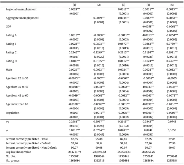
In terms of the relationship between credit defaults and business cycles, the models estimated in the two modalities provide basically the same evidence. However, the effects seem to be stronger in Consumer Credit transactions. Our interpretation is that, because Vehicle Financing loans usually have collateral, the rates of default in this modality are smaller and less responsive to business cycles than Consumer Credit transactions.
11%, the probability of default increases to 7%. If we include the other variables measuring business cycles, this effect becomes statistically insignificant. In the Vehicle Financing modality, despite of being statistically significant, the effect is still smaller.
Table 2: Marginal effect on default probability – Vehicle Financing modality
(1) (2) (3) (4) (5)
Regional unemployment 0.0024*** 0.0011*** 0.0011*** 0.0013*** (0.0001) (0.0001) (0.0002) (0.0001) Aggregate unemployment 0.0059*** 0.0048*** 0.0067*** 0.0062*** (0.0001) (0.0001) (0.0001) (0.0002)
GDP -0.0058*** -0.0061***
(0.0002) (0.0002) Rating A 0.0013*** -0.0008** -0.0011*** -0.0015*** -0.0054***
(0.0003) (0.0004) (0.0003) (0.0004) (0.0005) Rating B 0.0925*** 0.0893*** 0.0872*** 0.0863*** 0.0739*** (0.0013) (0.0012) (0.0013) (0.0013) (0.0010) Rating C 0.2245*** 0.2249*** 0.2210*** 0.2198*** 0.1911*** (0.0021) (0.0020) (0.0021) (0.0021) (0.0016) Rating D 0.8106*** 0.8105*** 0.8112*** 0.8124*** 0.7427*** (0.0016) (0.0015) (0.0016) (0.0016) (0.0015) Male 0.0024*** 0.0023*** 0.0024*** 0.0024*** 0.0032*** (0.0002) (0.0003) (0.0003) (0.0003) (0.0003) Age from 25 to 35 -0.0013*** -0.0007** -0.0008** -0.0008** -0,0005 (0.0003) (0.0004) (0.0004) (0.0004) (0.0005) Age from 35 to 45 -0.0038*** -0.0031*** -0.0032*** -0.0033*** -0.0038***
(0.0003) (0.0003) (0.0004) (0.0004) (0.0005) Age from 45 to 60 -0.0069*** -0.0061*** -0.0062*** -0.0063*** -0.0073***
(0.0003) (0.0004) (0.0004) (0.0004) (0.0005) Age more than 60 -0.0100*** -0.0089*** -0.0091*** -0.0091*** -0.0116***
(0.0004) (0.0005) (0.0005) (0.0005) (0.0007) Population 0.0001 -0.0013*** -0.0005*** -0.0005*** -0.0006***
(0.0001) (0.0001) (0.0002) (0.0002) (0.0002) σc 0.2981*** 0.2917*** 0.2915*** 0.2842*** 0,0745
(0.0101) (0.0096) (0.0102) (0.0104)
ρ 0.0815*** 0.0784*** 0.0783*** 0,0747 0,1655
(0.0051) (0.0047) (0.0050) (0.0051)
Percent correctly predicted - Total 87,85 95,88 87,85 87,85 87,85 Percent correctly predicted - Default 57,96 52,8 57,96 57,96 57,96 Percent correctly predicted - Non Default 90,07 99,08 90,07 90,07 90,07 Log-likelihood value -254211,74 -283792,62 -253573,23 -252951,29
-No. obs. 1750841 1928644 1750841 1750841 1750841
No. groups 1265684 1392716 1265684 1265684 1265684 Notes:
1) Models (1), (2), (3) and (4) are probits with unobserved individual component, and specification (5) is a linear probability model estimated by random effect estimation.
2) All models also include variables controling for the borrower’s occupation, interest rate and unobserved fixed effect of financial institution. 3) Standard errors are in parenthesis. Significance: ***=1%, **=5%, *=10%. 4) Probability of more than 50% is the criterium used to define predicted default.
influence in defaults than regional variables. Not only the impact of the aggregate unemployment is larger than that of the regional unemployment rate, but also, in the Consumer Credit modality, this second effect becomes statistically insignificant when we additionally introduce aggregate variables measuring business cycles in the model.
Similar conclusions about the effect of the business cycle on the probability of default emerge if we use GDP instead of unemployment as measure of economic activity. Our estimations suggest that one additional percentage point in the GDP growth rate reduces the probability of default in less than one percentage point. We should report, however, that more uncertainty is associated with this effect. In some other specifications we estimate, the GDP variable was not statistically significant, even though the point estimations preserve the magnitude of the effect.
Jointly, therefore, our results using data on the individual level show the same evidence obtained in the time series estimations of section 3: there is a significant relationship between business cycles and credit defaults, but the impact of the economic activity on delinquency rates in retail sector transactions seems to be limited. The unemployment rate effect, as well as the GDP effect, on the probability of default in these transactions appears to be modest. The magnitude of the impact of business cycles are still smaller in the Vehicle Financing modality.
Besides, our estimations provide some other interesting results. As already pointed out, the risk classifications of the banks are consistent and seem to capture the intrinsic risks of each transaction. The worse the risk rating of the transaction, the large is the estimated probability of default. For example, the probit estimations show that, in the Consumer Credit modality, a transaction classified as A has a probability of default around 20 percentage points larger, when compared to a transaction with rating AA; while a transaction rated as D has a probability approximately 90 percentage points larger. Despite the difference in the level, the same conclusion can be obtained from the probit estimations in the Vehicle Financing modality and from the linear probability model.
Tables 1 and 2 also report the standard deviation of the unobserved individual effect and the corre-lation between the composite latent errors,ci+ui,j,t, across any two time periods:ρ=σ2
c/(1 +σ
2
c).
This correlation is also the ratio of the variance ofcito the variance of the composite error (remember that the variance of the idiosyncratic error in the latent variable model is unity), and it is useful as a measure of the relative importance of the individual unobserved effect. Our probit estimations suggest that, in the Consumer Credit modality, the individual component accounts for more than 26% of the variance of the composite error. In the Vehicle Financing models this number is around 7%. Moreover, the absence of unobserved individual effects is statistically equivalent toH0 : σc2 = 0. Our results
show that we cannot reject this hypothesis in any of the usual significance levels, indicating that the presence of unobserved individual components cannot be neglected, as usually the literature on this issue seems to do.
Finally, one can also argue that the effect of these variables measuring business cycles on default events is not contemporaneous. Because of this argument, we carry out some other estimations for robustness check, including these variables lagged one period. We do not present the results here, but they all support the same conclusions just presented and can be provided under request.
5. CORRELATION AND TRANSITION MATRICES
reduce credit supply and further intensify the business cycles, as usually argued in discussions about procyclical effect of the Basel II Accord.
We adopt the historical approach to estimate default correlations and transition probabilities ma-trices in our data. By default correlation we mean the correlation between pairs of transactions with different (or equal) risk ratings jointly moving to the state of default. Our estimations are based on the methodology developed by Servigny and Renault (2002). These authors propose a way of extract-ing information about marginal and joint transitions between risk ratextract-ings from historical data without assuming any specific model for transitions. Gómez (2007), argue that this methodology has many important applications. Servigny and Renault (2002) worked with the Standard & Poor’s database and selected a sample covering only U.S. companies.
The methodology uses the cohort method, assuming the discrete time Markovian assumption. Specifically, loan transactions are grouped into risk ratings, and correlations between these ratings are calculated through transition probabilities. These transition probabilities are estimated under the assumption that the time series of classifications is a realization of a discrete time Markov chain, with states being the risk ratings. The transition probability from stateito statejis estimated by dividing the number of observed transitions fromitojin a given period by the total number of observations in stateiat the beginning of the period.
However, this method uses discrete time and therefore disregards intermediate transitions occurring within each period. Lando and Skodeberg (2002) consider this fact one disadvantage, when compared to other methods that consider continuous time. They report that null estimates for transition prob-abilities can be mistakenly obtained if the initial rating state is equal to the final state. Furthermore, transitions of transactions that do not stay in the dataset during the entire period, either because they were finished before the end of the period or because they were initiated after the beginning of the pe-riod, are not considered in the calculation. We hope dealing with this problem in future works, through the use of methods in continuous time, where the frequency of transition observations is minimized.
Keeping all these issues in mind, we proceed to use this method to empirically estimate default correlations. Details are given in which follows. First, marginal or univariate transition matrices are obtained from the frequencies of transitions between the risk ratings. In particular, we are interested in the probability of a given transaction moving from different risk ratings to the state of default. Univariate transition frequencies in one period are calculated by the following method:
fk i =
Tk i
Ni, (8)
where:
• fk
i is the marginal transition frequency from ratingito ratingkin one period;
• Tk
i is the total number of transactions moving from ratingiat the beginning of the period to
ratingkat the end of the same period;
• Niis the total number of transactions belonging to ratingiat the beginning of the period.
Similarly, joint or bivariate transition frequencies are estimated by:
fi,jk,l= Tk
i ∗Tjl
Ni∗Nj, (9)
where:
• fi,jk,lis the joint transition frequency from ratingsiandj, respectively to ratingskandl, in one
• Tk
i is the total number of transactions moving from ratingiat the beginning of the period to
ratingkat the end of the same period;
• Tl
j is the total number of transactions moving from ratingj at the beginning of the period to
ratinglat the end of the same period;
• Niis the total number of transactions belonging to ratingiat the beginning of the period;
• Njis the total number of transactions belonging to ratingjat the beginning of the period.
Specifically, we are more interested in the probabilities of two given transactions with, say, ratings
iandj, jointly moving to the default stated, i.e.,fi,jd,d.
We obtain these marginal and joint transition frequencies for each period. To obtain a measure of transition probabilities, we aggregate these period frequencies using as weights the number of trans-actions belonging to a certain rating at the beginning of each period relative to the total number of transactions belonging to that same rating at the beginning of all periods.
Then, the transition correlations between risk ratings are obtained by:
ρk,li,j =
fi,jk,l−f k i ∗fjl
q
fk
i ∗ 1−fik
∗fl
j∗ 1−fjl
,
(10)
where:
• ρk,li,j is the correlation coefficient between a pair of loans moving from ratingsiand j at the
beginning of one period respectively to ratingskandlat the end of the period.
We apply this methodology to our dataset of microdata. We estimate marginal transition probabili-ties, joint transition probabilities and default correlations in retail loans in the two modalities we have been using in this paper, adopting the traditional segmentation used in the literature, based on risk ratings. So, we split the transactions in five ratings (AA, A, B, C and Default) according to classifications of the two financial institutions.
Table 3 presents univariate transition probabilities for both Consumer Credit and Vehicle Financing modalities. First, the table shows that, in general, in both modalities the probability of staying in the same risk rating in which the transaction was in the last period (main diagonal of the matrices) is higher than the probability of changing. Therefore, for instance, the transaction that was rated as AA in a given period tends to continue in this risk rating in the next period. Second, this fact is particularly true for the state of default, which shows that this state is almost absorbing, i.e., once a loan moves to default, it nearly stays there forever. Third, showing the consistency of risk classification, in both modalities when the risk rating of a transaction gets worse, the probability of moving to the state of default also increases—for example, while the probability of an AA transaction moving to default is approximately 3%, the same probability of a C transaction is around 40%. Finally, consistent with Figure 3 in Appendix, Table 3 also shows that in general the probabilities of moving from any state to default (last column of matrices) are higher in Consumer Credit modality than in Vehicle Financing. This can be explained by the existence of collateral in the last modality, as already argued. Similar results were found in a previous paper of the last three authors.12
We also estimate the joint transition probabilities in both modalities. Because there are so many combinations and the results are hard to interpret, we only present them in Appendix. These joint transition probabilities are, however, necessary to obtain the default correlation matrices, as can be
Table 3: Univariate transition probabilities
Consumer Credit Final Rating
AA A B C Default
Initial
Rating
AA 48,29% 42,74% 2,52% 3,20% 3,24% A 1,26% 77,18% 11,61% 2,37% 7,58% B 0,07% 8,78% 60,12% 4,46% 26,58% C 0,13% 3,05% 8,48% 47,65% 40,69% Default 0,01% 0,51% 2,85% 0,79% 95,83%
Vehicle Financing Final Rating
AA A B C Default
Initial
Rating
AA 88,92% 1,81% 3,05% 2,88% 3,33% A 9,31% 76,44% 5,95% 4,00% 4,30% B 8,68% 18,25% 44,99% 10,74% 17,35% C 10,07% 11,51% 6,46% 34,35% 37,61% Default 2,75% 3,39% 1,80% 2,59% 89,47% Note: Average of semi-annual transition frequencies from rating i (initial rating) to ratingk(final rating), whereiandk= AA, A, B, C, Default. Period: Jan/2003 to Jul/2008.
seen in equation (10). The correlation matrix for Consumer Credit as well as for Vehicle Financing modality are presented in Table 4 below.
There is great dispersion in the estimated default correlations in both modalities. Similar results are found in the literature, where empirical papers show default correlations ranging from very negative to high positive values.13Default correlations are also found to be generally low in our data, which may be
possibly explained by the fact that our data come from the retail sector. In this segment loans are given to a large number of different individuals, which may lead to a diversification effect, thus spreading the influence among default events. Despite of being also generally low, the literature that uses corporate data reports that correlations should increase as ratings decrease, once low-rated companies are more susceptible to problems in the aggregate economy. The reasoning is that, if the economy experience a downturn, all companies close to the edge of default are more likely to experience solvency problems, which makes default events more correlated in these groups of transactions. Interestingly, we do not obtain higher correlations among low-rated individuals in our data, except for those already in default.
Table 4: Empirical default correlation matrices
Consumer Credit Vehicle Financing
AA A B C Default AA A B C Default
AA 1,67% 1,03% 2,40% -0,46% 2,27% 0,75% 0,51% 1,13% 0,47% -6,82% A 1,03% -2,77% -3,68% -3,63% -17,69% 0,51% 0,01% 0,23% 0,96% -0,83% B 2,40% -3,68% -3,07% -3,04% -22,83% 1,13% 0,23% 0,96% 1,12% -7,42% C -0,46% -3,63% -3,04% -6,34% 15,86% 0,47% 0,96% 1,12% -2,04% -20,40% Default 2,27% -17,69% -22,83% 15,86% 23,88% -6,82% -0,83% -7,42% -20,40% 32,86% Note: Default correlations calculated according to equation (8), using univariate default probabilities of Table 3 and bivariate default probabilities of Table 7 and 8. Period: Jan/2003 to Jul/2008.
We also estimate univariate transition probabilities in different phases of the business cycle. To define the periods of growth and recessions during the period covered by our data we rely on a recent
work of the Brazilian Institute of Economics of the Getulio Vargas Foundation (IBRE-FGV), which devel-ops a methodology to identify recessions and booming periods of the Brazilian economy—Committee on Business Cycle Dating, IBRE-FGV.14 According to the Committee, from January 2003 to July 2008,
except for the first semester of 2003, the Brazilian economy experienced a period of growth. Using this classification we split our dataset and estimate transition probabilities matrices for recessions and booming periods, which are reported in Table 5. As we would expect, in general the probability of moving from any risk rating to the state of default is larger in recessions than during expansions, in both modalities.
Table 5: Univariate transition probabilities – recession and booming
Consumer Credit - Recession Vehicle Financing - Recession
Final Rating Final Rating
AA A B C Default AA A B C Default
Initial
Rating
AA 40,03% 35,15% 3,35% 17,41% 4,07% AA 77,40% 12,62% 6,85% 1,66% 1,47% A 2,02% 61,06% 14,84% 8,58% 13,50% A 0,02% 84,40% 6,50% 3,40% 5,68% B 0,13% 9,52% 49,76% 6,44% 34,16% B 0,11% 22,46% 45,64% 7,59% 24,19% C 0,04% 0,74% 1,85% 56,45% 40,92% C 0,03% 23,45% 8,41% 14,82% 53,30% Default 0,00% 0,26% 0,68% 0,32% 98,74% Default 0,01% 4,08% 1,73% 1,66% 92,52%
Consumer Credit - Boom Vehicle Financing - Boom
Final Rating Final Rating
AA A B C Default AA A B C Default
Initial
Rating
AA 48,97% 43,36% 2,45% 2,04% 3,17% AA 88,92% 1,81% 3,05% 2,88% 3,33% A 1,25% 77,38% 11,57% 2,30% 7,50% A 10,28% 75,61% 5,89% 4,06% 4,16% B 0,07% 8,77% 60,24% 4,44% 26,48% B 9,29% 17,95% 44,94% 10,96% 16,87% C 0,14% 3,24% 9,03% 46,93% 40,67% C 10,50% 11,01% 6,37% 35,17% 36,95% Default 0,01% 0,52% 2,91% 0,80% 95,76% Default 2,92% 3,35% 1,81% 2,65% 89,28% Note: Average of semi-annual transition frequencies from ratingi(initial rating) to ratingk(final rating) in periods of recession and booming. Period: Jan/2003 to Jul/2008.
6. VALUE AT RISK EXERCISES
To analyze the impact of these increasing default probabilities and transition probabilities during periods of economic recessions on the portfolio losses, in this section we carry out some credit Value at Risk (VaR) simulation experiments. The portfolio we study is composed by retail loans based on the portfolio positions of the two selected institutions in March 2009.
Based on these data, we obtain estimates of credit VaR in two scenarios: periods of economic growth and recessions. The default probabilities and correlations estimated in the previous section are used as input parameters in the simulation of losses in each scenario. Because of the large number of trans-actions in the portfolio we have in hands, we decided to randomly chose a sample of 50 thousand transactions from this population, stratified by risk ratings, to compose our portfolio.
Then, we assigned a hypothetical unit value to each portfolio exposure. One hundred simulations of this hypothetical portfolio were performed in each simulation run, in a total of five runs. In each sim-ulation, binary variables (default or non-default) were sampled from a Bernoulli distribution, according to the parameters (default probabilities and correlations) estimated empirically for each risk rating.
We used a default-mode version of the CreditMetrics model, as presented in Gordy (2000), to sim-ulate future portfolio losses. By default-mode version we mean that only losses arising from default
events are considered in the model, i.e., losses associated with credit quality deterioration of the bor-rower are not considered in the model. This method is known in the literature as Simplified CreditMet-rics. The time horizon used in the simulation experiment is one semester.
The model structure is the following:
L=
N
X
i=1
EADi∗LGDi∗Yi, (11)
where:
• Lis the total portfolio loss at the end of the period (semester), equal to the sum of individual losses;
• Nis the number of transactions in the sample (50,000 in our simulation);
• EADiis the exposure at default for thei-th credit transaction (equal to R$1);
• LGDiis the loss given default for thei-th credit transaction;
• Yidefault indicator variable (Bernoulli) for thei-th credit transaction.
In our exerciseLGDi is a random variable with Beta probability distribution, whose parameters come from Silva et al. (2009b). We simulate the portfolio losses distribution for each of the two economic scenarios and obtain the VaR in each scenario for three percentiles (95%, 99% and 99.9%).
Table 6 below presents the estimated VaR for recessions and booming phases of the business cycles, for both modalities and the three percentiles considered. In general, the estimated losses in recessions are larger than those in expansionary periods. In Credit Consumer modality the difference is around 14% in every percentile, while in Vehicle Financing the losses are approximately 4% higher. The smaller VaR in Vehicle Financing, compared to that of the Consumer Credit, results from lower estimated prob-abilities and default correlations.
Table 6: Simulated Credit VaR
Consumer Credit
Percentiles 95,0% 99,0% 99,9%
Booming 18,85% 18,89% 18,91%
Recession 21,55% 21,61% 21,62%
Vehicle Financing
Percentiles 95,0% 99,0% 99,9%
Booming 12,27% 12,31% 12,32%
Recession 12,82% 12,88% 12,90%
Note: Percentiles of the simulated potential losses distribution. The VaR experiment is based in a portfolio composed by 50 thousand transactions sampled from portfolios of the two banks.
Results are based in one hundred simulations in five runs.
and Renault (2002) simulate a “typical" portfolio of one hundred non-investment grade bonds with unit exposure using the S&P dataset. They find a VaR for recession 45% higher than that of periods of growth. Trück and Rachev (2005) simulate the losses in a loan portfolio of a large European bank in two distinct periods of the business cycle. They obtain a VaR in periods of recession six times higher than that of expansionary years, and the VaR in recessions is more than twice the average VaR, considering the whole sample period.
In light of these results Trück and Rachev (2005) conclude that average values of default probabilities and correlations should not be used in models of credit risk, and the effect of the business cycle on these parameters, and hence on the VaR, is quite obvious to be overlooked. Likewise, Cowan and Cowan (2004) claim that, by not considering the impact of changes in the business cycle on the portfolio losses, the measure of credit risk will be underestimated and, consequently, so is the capital required to manage the underlying risks.
We also quote that understanding the impact of the business cycle on credit risks is crucial for both supervisors and lenders, once calculations of regulatory capital take into account parameters such as probabilities of default and default correlations, which can be influenced by the level of economic activity. However, our results show that, at least in the retail sector in Brazil, the difference in the losses along the business cycle seems to be smaller than that reported in the literature. But obviously other studies in this sector, and particularly in other credit modalities, need to be done to further extend our knowledge on this issue.
7. CONCLUSIONS
In this paper we analyze the relationship between credit defaults and business cycle using retail credit transactions. In particular, we are interested in the first part of the argument that suggests that the Basel II Accord might amplify fluctuations in business cycles. The reasoning of this argument is that economic recessions increase credit default and the losses in portfolios of lender institutions, which require a recomposition of capital requirements, causing an increase in the cost of capital and a reduction in credit supply that further intensifies the economic downturn. However, we do not study in this paper the second part of this argument, i.e., if this increase in credit default, in the losses of portfolios and the consequent recomposition of capital requirements cause a shrinking in credit supply. As already emphasized, the difficulty of this task is to separate credit supply from credit demand and this can be the object of another study.
We explore the evidence coming from time series data as well as the evidence provided by data on the individual level. The results suggest that there is a significant relationship between credit defaults and business cycles, but this relationship is less strong than previously pointed out by other studies. We also find that in general women default less than men, and the older the borrower, the lower is the probability of delinquency.
First, our time series evidence suggests that after a positive shock in the unemployment rate, iden-tified by a Vector Autoregressive (VAR) model, credit default in retail transactions increase, but this increase is modest and short lasting. Second, the estimations based on the microdata also provide evi-dence that the impact of an increase in the unemployment rate (both aggregate and sectoral) or in the GDP growth rate is small. While an additional percentage point in sectoral unemployment rate and in aggregate unemployment rate seems to produces an increase in the probability of default in Consumer Credit transactions in, respectively, 1 and 3 percentage points, the same increase in the GDP growth rate increases this probability in less that one percentage point.
only 4% higher in Vehicle Financing modality, when compared to the losses during booming periods. These values are much lower than those found in recent papers.
Most of studies in the literature reporting large impacts of recessions on the probability and cor-relations of default, and on the potential losses in portfolios of lender institutions concentrates on corporate data. Even though additional studies about this issue are obviously needed, in particular studies focusing on the effects of the Basel II Accord on the credit supply during recessions, our results suggests that, in retail sector in Brazil, the effects of the first part of the mechanisms that are argued to generate procyclical forces are modest. We suggest that these results can be possibly explained by the fact that, in the retail sector, loans are given to a large number of individuals, which may help to diversify the influence of default events. It is worth mentioning that our results definitely do not indicate that procyclical effects do not exist. After all, retail sector represents only part of the credit market. Second, we do not study the second part of the argument, which has to do with credit supply. And our intuition says that all these features regarding the balance sheets of the banks, combined with concerns during recessions about future developments of the economy in the short and medium run, can have stronger effects through credit supply. Therefore, more research must be done, specially on the mechanisms driving credit supply.
BIBLIOGRAPHY
Allen, L. & Saunders, A. (2002). A Survey of Cyclical Effects in Credit Risk Measurement Models. Technical report, Stern School of Business, New York University.
Bangia, A. (2002). Ratings Migration and the Business Cycle with Applications to Credit Portfolio Stress Testing. Journal of Banking and Finance, 26:445–474.
Basle Committee on Bank Supervision (2001). The New Basel Capital Accord. Report, Bank of Interna-tional Settlements, Basle.
Caouette, J., Altman, E., & Narayanan, P. (1998). Managing Credit Risk. The Next Great Financial Chal-lenge. New York: Wiley.
Cowan, A. & Cowan, C. (2004). Default Correlation: An Empirical Investigation of a Subprime Lender. Journal of Banking and Finance, 28:753–771.
Gómez, J. (2007). An Alternative Methodology for Estimating Credit Quality Transition Matrices. Tech-nical report, Borradores de Economía, Banco de La Republica de Colombia.
Gordy, M. (2000). Comparative Anatomy of Credit Risk Models. Journal of Banking and Finance, 24:119– 149.
Jarrow, R. A. & Turnbull, S. (2000). The Intersection of Market and Credit Risk. Journal of Banking and Finance, 24:271–299.
Kashyap, A. & Stein, J. (2004). Cyclical Implications of Basel II Capital Standards, Federal Reserve Bank of Chicago. Economic Perspectives, 1st Quarter:18–31.
Koopman, S. & Lucas, A. (2005). Business and Default Cycles for Credit Risk.Journal of Applied Economet-rics, 20:311–323.
Koopman, S., Lucas, A., & Klassen, P. (2005a). Empirical Credit Cycles and Capital Buffer Formation. Journal of Banking and Finance, 29:3159–3179.
Lando, D. & Skodeberg, T. (2002). Analyzing Rating Transitions and Rating Drift with Continuous Obser-vations. Journal of Banking and Finance, 26:423–444.
Lucas, D. (1995). Default Correlation and Credit Analysis. Journal of Fixed Income, 4(4):76–87.
Merton, R. (1974). On the Pricing of Corporate Debt: The Risk Structure of Interest Rates. Journal of Finance, 29:449–470.
Nagpal, K. & Bahar, R. (2001). Measuring Default Correlation. Risk, 14:129–132.
Nickell, P., Perraudin, W., & Varotto, S. (2000). Stability of Rating Transitions. Journal of Banking and Finance, 24 (1-2):203–227.
Repullo, R., Saurina, J., & Trucharte, C. (2009). Mitigating the Procyclicality of Basel II. CEPR Discussion Paper 7382.
Repullo, R. & Suarez, J. (2008). The Procyclical Effects of Basel II. CEPR Discussion Paper 6862.
Rosch, D. (2003). Correlations and Business Cycles of Credit Risk: Evidence from Bankrupticies in Ger-many. University of Regenburg.
Saurina, J. & Trucharte, C. (2007). An Assessment of Basel II Procyclicality in Mortgage Portfolios.Journal of Financial Services Research, 32:81–101.
Servigny, A. & Renault, O. (2002). Default correlation: Empirical evidence. Technical report, Standard and Poors.
Silva, A. C. M., Marins, J. T. M., & Neves, M. B. E. (2009a). Loss Given Default: um Estudo sobre Perdas em Operacões Prefixadas no Mercado Brasileiro. Working Paper Series, Banco Central do Brasil.
Silva, Silva, A. C. M., Marins, J. T. M., & Neves, M. B. E. (2009b). The Influence of Collateral on Capital Requirements in the Brazilian Financial System: an Approach Through Historical Average and Logistic Regression on Probability of Default. Working Paper Series, Banco Central do Brasil.
8. APPENDIX A
Figure 3: Credit default based on microdata, semiannually
0% 2% 4% 6% 8% 10% 12% 14% 16% 18%
2
0
0
3
.1
2
0
0
3
.2
2
0
0
4
.1
2
0
0
4
.2
2
0
0
5
.1
2
0
0
5
.2
2
0
0
6
.1
2
0
0
6
.2
2
0
0
7
.1
20
07
.2
2
0
0
8
.1