Delivery System
Marta Fernandes, Paulo Oliveira, Susana Vieira, Luís Mendonça, João Lemos Nabais and Miguel Ayala Botto
Abstract Water is a vital resource and the growing populations and economies around the globe are pushing its demand worldwide. Therefore, the water conveyance operation should be well managed and improved. This paper proposes the develop-ment of reliable models able to predict water levels of a real 24.4 km water delivery channel in real time. This is a difficult task because this is a time-delayed dynamical system distributed over a long distance with nonlinear characteristics and external perturbations. Artificial neural networks are used, which are a well-known model-ing technique that has been applied to complex and nonlinear systems. Real data is used for the design and validation of the models. The model obtained has the ability to predict water levels along the channel with minimum error, which can result in significant reduction of wasted water when implementing an automatic controller.
Keywords Data based modeling
⋅
Water delivery systems⋅
Artificial neural net-works⋅
Nonlinear autoregressive exogenous model1
Introduction
Water is the most important resource for human life therefore it has to be efficiently managed. An increase of 55 % in global water demand is expected by 2050, mainly influenced by the projected growing demands from manufacturing, thermal electric-ity generation and domestic use [1].
M. Fernandes (
✉
)⋅ P. Oliveira ⋅ S. Vieira ⋅ L. Mendonça ⋅ J.L. Nabais ⋅ M.A. Botto IDMEC, LAETA, Instituto Superior Técnico, Universidade de Lisboa,Lisbon, Portugal
e-mail: marta.fernandes@tecnico.ulisboa.pt L. Mendonça
Department of Marine Engineering, Escola Superior Náutica Infante D. Henrique, Oeiras, Portugal
J.L. Nabais
School of Business Administration, Polytechnical Institute of Setúbal, Setúbal, Portugal
© Springer International Publishing Switzerland 2017 P. Garrido et al. (eds.), CONTROLO 2016, Lecture Notes
in Electrical Engineering 402, DOI 10.1007/978-3-319-43671-5_24
The development of models and the design of controllers for irrigation channel systems has been a difficult task since these systems are distributed over long dis-tances and present a dynamic behavior characterized by time delays, strong nonlin-earities, unknown perturbations and numerous interactions among sub-systems [2]. Control of irrigation channels has been driving the attention of engineers since immemorial times and several papers have been published in this field [3–12]. One of the most accepted and used models for simulation of the physical dynamics of a real main irrigation channel pool is the system described by the Saint-Venant equa-tions [13]. However, the difficulty in determining the parameters of these equations remains as one of the main drawbacks of this physically oriented modeling approach. As a consequence, new alternative modeling approaches, namely both parametric and nonparametric data-driving models, have been proposed, in which the model parameters are optimized to match real data [14].
The water delivery system which the authors intend to model is the Milfontes Canal, a large scale open water channel supplying water to the village of Vila Nova de Milfontes as well as to local farmers. The facilities are equipped with a basic monitoring system that provides information on the water depth and gate aperture levels along the channel. The absence of an automatic control system together with the necessity of ensuring the clients’ water requests results in large amounts of wasted water at the end of the channel.
As far as the authors are aware of, Artificial Neural Networks (ANN) have never been applied to real irrigation channels in normal operation. In this paper, ANN are employed to create a nonlinear dynamic model of the Milfontes Canal using real operation data from 2013. This model has the ability to predict future water levels along the infrastructure, from the perspective of signal prediction in real time. Well-known performance measures are used to assess the models performance. The model developed may ensure a significant reduction of wasted water when implementing an automatic controller.
The paper is organized as follows. In Sect.2, the system modeling is addressed. The results obtained are shown and discussed in Sect.3and conclusions are drawn in Sect.4.
2
Artificial Neural Networks
ANN are self-organizing systems, having the ability to learn from examples, that is, to be trained with provided data. This feature makes them extremely useful to model complex or unfamiliar systems, since it does not require system in-depth knowledge from the designer. Usually, ANN modeling follows three steps: structure identifica-tion, parameter estimation and model validation.
The system to be identified can be represented as a Input Multiple-Output (MIMO) Nonlinear Auto Regressive with exogenous inputs (NARX) model:
where x is a state vector obtained from input-output data and y the system output. In this case, the state vector x at each time step k can be obtained from the inputs and outputs of the system, joining them in a vector:
x(k) = [y1(k), … , y1(k − p1+ 1), … , yp(k), … , yp(k − pp+ 1), u1(k), … , u1(k − m1+ 1), … ,
um(k), … , um(k − mm+ 1)]T.
(2)
The parameters m1, … , mmare the orders of the inputs u1, … , um, and the
para-meters p1, … , ppare the orders of the outputs y1, … , yp, respectively. Note that the
dimension of the state vector is given by D =∑mj=1mj+
∑p
j=1pj[15]. For a dynamic
system using this state vector, the model is represented by:
̂y(k + 1) = f (x(k)) (3)
The state variables x are called the regressor and the predicted outputs ˆy the regressand.
In the present case, the system model will take the form of a neural network and the tuning mechanism is known as training the network. This training consists on adjusting the network parameters the connection weights and the node biases accord-ing to an error backpropagation algorithm.
In this type of problems, data is usually divided for model training and testing. Training a neural network model is based on a learning algorithm. For this work, the Levenberg-Marquardt backpropagation algorithm is employed. The performance measures used were the mean square error (MSE) for both model training and testing. Mean absolute error (MAE) and mean absolute relative error (MARE) were used as well to assess the performance of model testing.
3
Results and Discussion
3.1 System Configuration
A schematic representation of the system inputs and outputs used in the system iden-tification procedure is presented in Fig.1. The group of major offtakes (u2to u7) plus the flow rate entering the channel inlet (u1) are the inputs of the system, in a total
of 7. The outputs consist on two types of sensors, in a total of 10: upstream (y1, y4,
y7 and y10) and downstream (y3, y6 and y9) water depth sensors and gate aperture
Fig. 1 Schematic representation of the channel inputs and outputs
3.2 Database
In order to carry out this work, the Associação de Beneficiários do Mira (ABM), a non-profit organization in charge of this hydro agricultural infrastructure, provided the database files. These files contained the sensor measurements plus a client order book containing the water requests during 2013, which were considered as the effec-tive outflows of the channel.
A procedure was applied in order to import the data from the database files into well-formatted datasets. All data points considered as outliers were removed. An outlier data point consisted on all negative values and all values that stood out by differing more than 15 units from their precedent. For the datasets, upon missing data, all the identified missing segments were recovered when possible using the zero order hold (ZOH).
Lack of either sensor or flow rates information reduced the list of potential datasets to the ones depicted in Table1. The information regarding the number of data points before and after outliers removal and missing data processing is pre-sented for each dataset. The percentage of missing data here prepre-sented represents the number of missing data points considering the total number of data points of each dataset.
It was verified that the sampling times of the sensors signals were not constant, usually falling in the 65–100 s range. Furthermore, the signals were not synchro-nized, therefore requiring further data processing. After signal processing, it was found that the time step, k, should be 90 s in order to take advantage of the available data provided by ABM.
Table 1 Final datasets obtained after identification of missing data and outliers and reconstruction with ZOH
Dataset ID Data points before
Missing data (%) Number of outliers
Data points after
49 6200 5.5 0 6199
50 6203 0.0 168 6203
51 6202 0.0 1 6202
3.3 System Delay
The system delay associated with the channel arises from the fact that the water levels do not immediately change when the water flow rates inwards and/or outwards of the channel are adjusted. Hence, the computation of the system delay has to take into account the location of the offtakes to estimate the delay caused by the time the water takes to arrive to the place where these offtakes are located.
According to tests performed on a site visit, the water speed on the channel was about 2.7 m/s. Considering the total length of the channel, the delay from the chan-nel’s intake flow to the water level measured on the other end of the channel was approximately 100 time steps, which translates to about 2 and a half hours.
The followed approach consisted on using an input-output delay as parameter of the system where the delay due to water flow rates was the same as the one in the water levels.
Given that the system delay may be set by many data points that situation would inevitably lead to an impracticable network model. In order to overcome this prob-lem, a subset of the past data up to the system delay (100 time steps) was fed into the model. In terms of time steps, that corresponded to the set of delays𝜏 = [1, 11, 21, 31, 41, 51, 61, 71, 81, 91, 101], with a time step of 5× k, which translates to 7.5 min.
3.4 Model Parameterization, Training and Validation
Regarding the model parameterization, the number of hidden layers and neurons in each layer were varied. In order to reduce variability and to find the best model, ten rounds of the same model were performed with different random initializations of network input weights. This was performed for each possible system delay, from 1 step to 100 time steps in time. The final system delay found corresponded to the model with best performance overall.
In this paper, the software Matlab® 2014a default stopping conditions were used, except for the training epochs, which were set to 200. The model training dataset was divided using the function divideblock from Matlab, where 70 % of data was used for train, 15 % for validation and 15 % for test. A linear autoregressive model with exogenous inputs (ARX) was estimated with the same regressor as the NARX networks for comparison, using the default conditions of ARX function from Matlab. The same subsets for train and test were used and the system delay was varied as performed for the NARX models.
Fig. 2 Channel inlet flow rates corresponding to input
u1for the datasets used for model training (Dat 49, 51 and 53) and testing (Dat 50)
3.5 Modeling Results
The model training dataset was obtained by joining datasets 49, 51 and 53. Each one of these datasets represent, respectively, a low, medium and high range of the variability that can be found in the system. The criterion for defining this variability was based on the flow rates values of the channel main inlet, u1, as it can be confirmed
in Fig.2. Dataset 50 was selected for test, given that it represents a medium range, considered suited for testing the model. In Fig.2, the lack of data between datasets 51 and 53 corresponds to a dataset which was not used for system modeling due to significant percentage of missing data.
The average performances of the best NARX and ARX models as well as of the NARX models obtained over the 10 rounds, are presented in Table2. The NARX model has a better performance than the ARX. Therefore, only the performance results of the best NARX model are presented for each output in Table3. This best model configuration was a single hidden layer with 10 neurons. More or less neurons in the hidden layer resulted in worst results, which happened as well when adding more layers.
The system delay found was 11 time steps which corresponds to approximately 16 min. This system delay is a result of a balance between the delays caused by the
Table 2 Models average performance results, for a 16 min delay, where the best model results are presented in more detail in Table3
MIMO models MSE (cm2) MAE (cm) MARE (cm)
10 rounds (NARX) 0.12± 0.01 0.16± 0.01 0.01± 0.01
Best NARX 0.11± 0.09 0.14± 0.08 0.01± 0.01
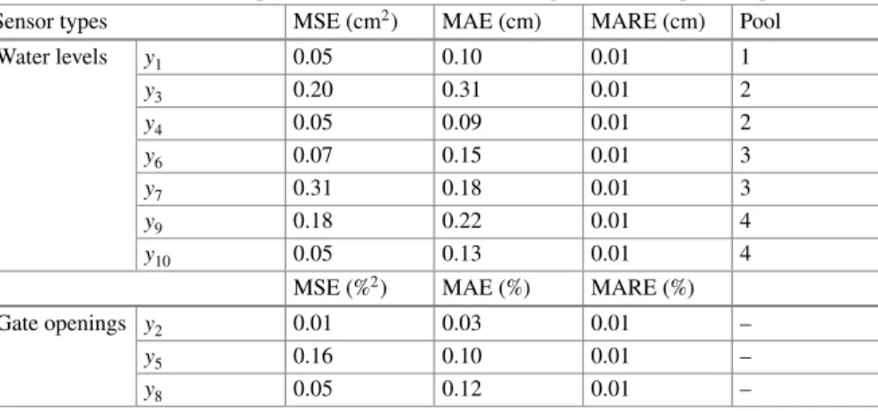
Table 3 Best NARX model performance results for each output and correspondent pool
Sensor types MSE (cm2) MAE (cm) MARE (cm) Pool
Water levels y1 0.05 0.10 0.01 1 y3 0.20 0.31 0.01 2 y4 0.05 0.09 0.01 2 y6 0.07 0.15 0.01 3 y7 0.31 0.18 0.01 3 y9 0.18 0.22 0.01 4 y10 0.05 0.13 0.01 4
MSE (%2) MAE (%) MARE (%)
Gate openings y2 0.01 0.03 0.01 –
y5 0.16 0.10 0.01 –
y8 0.05 0.12 0.01 –
channel intake flow rates and offtakes. The delay of each input or output depends on its location, therefore the delay caused by a flow rate located at the beginning of the channel is not the same as one at the middle or at the end.
Compared to the other outputs correspondent to the water levels, the output cor-respondent to downstream pool 3, y7, presents the higher MSE. The output of water level measured upstream pool 4, y9also presents a high error.
It is worth noting that both the water level outputs y7and y9are located, respec-tively, immediately before and after the gate that separates both pools 3 and 4, thus the cause to obtain these errors may be due to noise, a failure in the sensors measure-ment. The water level sensor represented by y3also presents a high MSE and MAE values, which may be due to the same cause. Regarding the remaining outputs, the model has the ability to predict one step ahead the water levels and the gate apertures with a minimum error. The best prediction model is presented in Figs.3,4,5and6, for each pool of the channel.
Fig. 3 Pool 1 downstream
model response RealMode
0 1000 2000 3000 4000 5000 6000 211 212 213 214 215 Time steps Water Levels [cm]
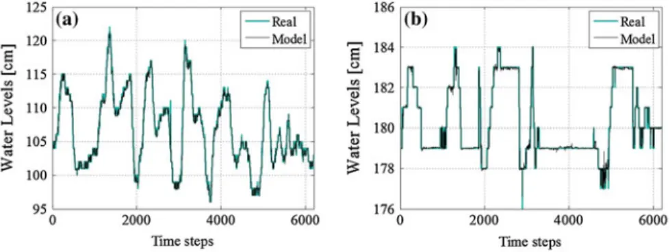
Fig. 4 Pool 2 model response: a upstream, b downstream
Fig. 5 Pool 3 model response: a upstream, b downstream
Fig. 6 Pool 4 model response: a upstream, b downstream
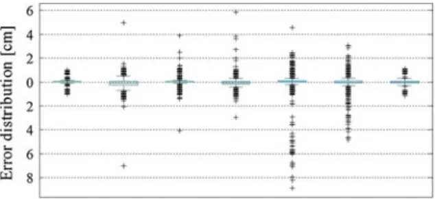
When analysing the prediction model results, it can be observed that the main sys-tem dynamics are being predicted correctly. Indeed, the great majority of the relative error values are within the 5 cm band, which may be better visualized in Fig.7.
As previously referred, the model presents higher prediction error when predict-ing water levels in pool 3. An approximate maximum error of almost 9 cm can be
Fig. 7 Model prediction errors distribution for each pool: upstream (Up) and downstream (D)
visualized when analyzing Fig.7, which is caused by an isolated spike in the output prediction. The occurrence of such phenomenon may indicate the used network is unable to model a minor system mode. For instance, it may be the case that the used network is not able to model the reflected water waves effect. Other complex flow phenomena may explain this behavior. Not to mention that noise is surely present in the real value measurements.
4
Conclusions
In this work, artificial neural networks were employed to model a real large scale water channel, using real operation data. This model has the ability to predict future water levels along the infrastructure in real time and in the future it may be used in a planning perspective, for control design or as an assistance tool for a FDI system. The best one step ahead prediction NARX model parameterization presented con-sists on a single-layered network with 10 neurons and a delay of approximately 16 min. The performance achieved by this model parameterization was equivalent to a MSE mean of 0.11± 0.09 cm2, which is considered reasonable given that the average real values range between 85 and 250 cm. The absence of other models of the same channel precludes a well-supported validation of the proposed model. Nev-ertheless, an independent test dataset, not used to train the models, was used with the purpose of validating them.
The application of neural network models to water delivery systems proved to be a good opportunity to show the benefits and features of using these type of black-box models. As a result, in the future the water waste at the end of the channel can be significantly reduced when applying an automatic controller, assisted by the model obtained in this paper.
Acknowledgments This work is supported by the Fundação para a Ciência e a Tecnologia (FCT), through IDMEC, under LAETA Pest-OE/EME/LA0022, and supported by the project PTDC/EMS-CRO/2042/2012. Susana Vieira acknowledges the support by the Program Investigador FCT (IF/00833/2014) from FCT, cofunded by the European Social Fund (ESF) through the Operational Program Human Potential (POPH).
References
1. Water, U.: The United Nations World Water Development Report 2014: Water and Energy. UNESCO, Paris (2014)
2. Malaterre, P., Baume, J.: Modeling and regulation of irrigation canals: existing applications and ongoing researches. In: IEEE International Conference on Systems Man and Cybernetics, vol. 4, pp. 3850–3855. Institute of Electrical Engineers Inc. (IEEE) (1998)
3. Zimbelman, D.D., Bedworth, D.D.: Computer control for irrigation-canal system. J. Irrig. Drainage Eng. 109(1), 43–59 (1983)
4. Mareels, I., Weyer, E., Ooi, S.K., Cantoni, M., Li, Y., Nair, G.: Systems engineering for irri-gation systems: successes and challenges. Annu. Rev. Control 29(2), 191–204 (2005) 5. Weyer, E.: System identification of an open water channel. Control Eng. Pract. 9(12), 1289–
1299 (2001)
6. Weyer, E.: Control of irrigation channels. IEEE Trans. Control Syst. Technol. 16(4), 664–675 (2008)
7. Eurén, K., Weyer, E.: System identification of open water channels with undershot and overshot gates. Control Eng. Pract. 15(7), 813–824 (2007)
8. Karunanithi, N., Grenney, W.J., Whitley, D., Bovee, K.: Neural networks for river flow predic-tion. J. Comput. Civ. Eng. 8(2), 201–220 (1994)
9. Vieira, S., Sousa, J., Durao, F.: Fuzzy modelling strategies applied to a column flotation process. Miner. Eng. 18(7), 725–729 (2005)
10. Lourenço, J., Botto, M., et al.: Modular modeling for large scale canal networks. In: 10th Por-tuguese Conference on Automatic Control, Funchal, Portugal, pp. 347–352 (2012)
11. Nabais, J., Duarte, J., Botto, M., Rijo, M.: Flexible framework for modeling water conveyance networks (2011). In: 1st International Conference on Simulation and Modeling Methodolo-gies, Technologies and Applications (SIMULTECH 2011), pp. 142–147, Noordwijkerhout, The Netherlands (2011)
12. Nabais, J.M.L.C., Botto, M.A.: Linear model for canal pools. In: 8th International Confer-ence on Informatics in Control, Automation and Robotics, ICINCO 2011, vol. 1, pp. 303–313, Noordwijkerhout, The Netherlands (2011)
13. Rivas-Perez, R., Feliu-Batlle, V., Castillo-Garcia, F., Linarez-Saez, A.: System identification for control of a main irrigation canal pool. In: Proceedings of the 17h International Federation of Automatic Control (IFAC) World Congress, Seoul, South Corea, vol. 17 Part 1 (2008) 14. Zhuan, X., Xia, X.: Models and control methodologies in open water flow dynamics: a survey.
In: AFRICON 2007, pp. 1–7. IEEE (2007)
15. Sousa, J.M., Kaymak, U.: Fuzzy decision making in modeling and control, vol. 27. World Scientific (2002)