A PARAMETRIC APPROACH TO ESTIMATE THE GREEN BOND
PREMIUM
STEPHAN JAKOB SCHMITT, 2486
Project carried out in the Master in Finance Program, under the supervision of:
Professor Pedro Lameira
Professor Adhemar Villani Junior
A Parametric Approach to Estimate the Green Bond Premium
ABSTRACT
We analyze whether green bonds are traded on a premium versus conventional issuances of the same issuer. We estimate the difference in yield between a sample of 160 green bonds and a synthetic conventional bond with identical characteristics. The paper finds that green bonds have been traded on slightly higher yields than conventional bonds. This premium seems to decline in 2016 and 2017. Our data suggests that there is no significant difference between the developed and emerging markets and between different industry groups.
Keywords: Green Bonds, Green Bonds Premium, Sustainable Investing, Government Bonds, Corporate Bonds.
I. Introduction
In January 2017, the French government entered the green bond market by issuing a 22-year OAT green bond with a record sale of 7 billion Euro. The overall demand exceeded the volume of the issuance by 23 billion Euro. According to one of the initial investors Carl Haarnack, fixed income portfolio manager at Actiam, the pricing was comparable with a non-green bond. The proceeds of one of the biggest and longest green bond in the market so far will be used to fund the “Invest for the Future” program of the French government. “Invest for the Future” aims to raise funds to fight and adapt to climate change, protect biodiversity and reduce pollution1. Due to its size and maturity,
the green OAT can be considered as the entry of sovereigns into the green bond market, which has been dominated by corporate and financial issuers so far.2 Going forward, the size of the OAT will
only be a glimpse of the future of the green bond market.
The issuance volume of green bonds shows a clear picture of its potential as the figures have been growing exponentially in the last four years. The amount outstanding of newly issued green bonds increased six-fold between 2013 and 20163 and seems to continue at a similar pace in 2017. An
increasing number of financial firms as well as China entering the market in 2016 have been driving this development. Corporate issuances are slowly contributing with companies like Apple and Hyundai who have recently accessed the market. The biggest non-financial issuers as reported by
1 State that the expenditure fall under the Eligible Green Expenditure and the AGF will issue two annual reports on the
use of the proceeds.
2 The first sovereign issuing a green bond was Poland with a smaller 750 million Euro bond in April 2016.
3 From 15.4 billion USD in 2013 to 95.1 billion USD in 2016 in Labelled Green Bonds per Bloomberg New Energy
Bloomberg New Energy Finance (BNEF) remain more traditional players like the energy companies Southern Powers and Iberdrola. However, in relation to the size of the entire fixed income market the total volume of green bonds issuances is still negligible – the potential seems far from reached.
Essential to the expansion of the green bond market is the classification of what is considered a green bond. According to BNEF (2017), green bonds are fixed income instruments of which the proceeds are used to finance projects and activities that promote climate change mitigation or adaptation, or other environmental sustainability purposes. The Green Bond Principles, introduced in 2014 and regularly updated, have established as a standard for considering what is a green bond. The Green Bond Principles published by ICMA (2017) are based on four pillars: use of proceeds, project evaluation and selection, management of proceeds and reporting. The guidelines are being used to avoid the practice of Greenwashing4. Consequently, within the green bond market, several
levels of environmental and sustainable benefits can be found in the use of the proceeds – the so-called ‘Shades of Green’.
Within this work, the aim is to answer the question whether yields of green bonds are lower than those of their conventional counterparts. If this thesis proves as true, firms investing in environmental or sustainable activities could use the size of the fixed income market to lower capital cost. For example, the energy sector with capital intense projects such as off- or onshore wind parks could widely benefit. In general, issuers profit from the reputational gains the disclosure
4 ‘Greenwashing’ is the artificial labelling of bonds as green to receive the benefits connected to green bond issuance
requirements of green bonds come along with. In other words, the second party opinion, which is used by most green bond issuers, helps to reduce information asymmetry with investors and align financial and sustainability guidelines.
Further benefits of green bonds also include the assets’ lower exposure to environmental risk compared non-environmental-screened issuances. According to Preclaw and Bakshi (2015), if the standards of green bonds can be developed further, and ‘Shades of Green’ become easier and cheaper to select, green bonds could be used to hedge environmental risk.
Nevertheless, the central question remains, whether investors are using conventional pricing or overpay for green bonds compared to conventional bonds with the same cash flows. Looking back, the heterogenous market of different issuers, shades of green, sectors and institutions has made it difficult to find a satisfying answer. Apart from Preclaw and Bakshi (2015) and Zerbib (2016), there have only been a few academic approaches to determine the existence of a green bond premium.
We aim to find answers and a method to estimate whether a green bond premium exists. To compute the possible green bond premium, we calculate the yield of a synthetic conventional bond with the same characteristics as the green bond. The spread between the yield of the green bonds and the synthetic conventional bonds reflects for the green bond premium.
The remainder of the study is structured as followed: Section II reviews literature on the green bond premium, impact of environmental performance on bond yields and parametric yield curve estimations. Section III introduces the methodology and describes the data. Section IV contains the empirical result and Section V concludes and summarizes the main results.
II. Literature Review
a. Environmental Management and the Green Bond Premium
The impact of environmental management on the cost of financing has been researched thoroughly. For example, Bauer and Hann (2010), Schneider (2011) and Sharfman and Fernando (2008) show that proactive environmental risk management lowers the cost of debt and increases credit rating. Graham, Maher, and Northcut (2001) and Graham and Maher (2006) associate environmental liabilities or scandals with decreasing bond ratings and increasing yields. Schneider (2011) shows that in the U.S. Pulp and Paper and Chemical industries aside from reputational gains when implementing environmental risk management, good environmental management lowers the probability of future clean-up costs due to the strengthening of environmental regulations. Additional research shows that the constitution of investors differs between environmental profiles. Chava (2014) indicates that those firms excluded from environmental screens have lower institutional ownership and less banks participating in their loan syndicates.
The literature targeting green bond specific determinants is less extensive. Preclaw and Bakshi (2015) are estimating the green bond premium with a cross sectional regression of yields while controlling for characteristics such as on-the-run vs. off-the-run bonds and credit rating. The author finds that green bonds are, according to the estimated model, traded with an average of 16.7 bps lower yields (as of August 2015) than conventional bonds. However, the only period where the authors found this significant difference is in the subsample between March 2015 and August 2015. The authors claim, that this might be due to the increasing sample size of green bonds. Preclaw and Bakshi (2015) point out three possible reasons for this premium: First, the persisting difference between supply and demand. Second, the usage of green bonds as a hedging tool for environmental
risk. Lastly, purely out of investor preferences for environmental friendly assets. Their report did not draw any conclusion about the origin of their premium.
Zerbib (2016) analyses the issuance specific premium of green bonds. The author matches a green bond with two conventional bonds of the same company with similar characteristics, interpolating between the yield of the two conventional bonds. This method has been used by Longstaff and Schwartz (1995) to calculate the cost of liquidity by comparing the yields of Credit Default Swaps (CDS) with corporate bonds. Zerbib (2016) is implementing a fixed-effects panel regression using the bid-ask spread and the number of zero-trading days as a proxy for liquidity to calculate the bond specific premia. Zerbib's (2016) results imply the overall premium of -8bp, which however is only significant to the 11% significance level. The author finds a negative premium of -11bp in the USD-denominated bonds, but no premium in Euro-issued bonds. Additionally, the author points out that the average green bond premium for bonds below an AAA-rating is significantly different from zero to a 10% significance level. Zerbib (2016) concludes that the riskier the bond is, the higher the green bond premium.
b. Term Structure Estimation Methods
Critical in the analysis of the existence of a green bond premium is to find either an identical “twin” of the bond or to control for the difference between bonds. Whereas Preclaw and Bakshi (2015) include several control dummies in their regression to account for difference, Zerbib (2016) aims to generate a “twin” by interpolating the yields of two closest comparable conventional bonds. We aim to find this “twin” by calculating the term structure of interest rates and pricing the cashflows of the green bond with spot rates of comparable conventional bonds. The advantage of this method is, as Gürkaynak, Sack, and Wright (2007) suggest, that it helps to smooth through idiosyncratic
variation of bond prices or yields. To calculate the spot rates of the mainly coupon paying bonds, we need to impose a structure to the zero-coupon curve.
In literature several smoothing methods are used. Fisher, Nychka, and Zervos (1995) fit cubic splines to the forward rate function and implement a smoothness penalty to ensure shape. McCulloch (1975) tailors a cubic spline to the discount function and adds a similar smoothness penalty. Nelson and Siegel (1987) propose a parametrical model to estimate a spot rate curve. The authors fit an exponential approximation of the discount rate directly to the prices. This is done by estimating four parameters defining the shape of the spot rate curve. The Nelson-Siegel model (NS) considers the main characteristics of yield curves as being monotony, a hump and its S-shape. Gürkaynak, Sack, and Wright (2007) find that Nelson-Siegel has difficulties fitting the longer maturities. Svensson (1994) extends NS by effectively adding a second hump term to the model. In this extension, six parameters need to be estimated. Gürkaynak, Sack, and Wright (2007) find that Nelson-Siegel-Svensson (NSS) increases the flexibility of the yield curve and captures the convexity of the yield curve better than NS. Gilli, Große, and Schumann (2010) claim that the estimation of NSS compared to NS is more stable and avoids so called ‘catastrophic jumps’ in the estimation of the parameters.
Diebold and Li (2006) use another variation of the NS framework to forecast yield curves. The authors fix one of the parameters in the NS equation to estimate the remaining of the 𝛽’s via the ordinary least square method (OLS). The rationale behind the choice of the value for 𝜆 is that 𝜆 determines the maturity at which the curvature of the curve reaches the maximum. This value can be chosen empirically. In addition, the authors determine that the three parameters 𝛽 , 𝛽 and 𝛽 can be interpreted as level, slope and curvature, respectively. Diebold and Li (2006) limit the
computational capacity needed for the estimation, OLS however, is only applicable if either spot-rates are available or no issuances are paying coupons.
NS and NSS have been used in wide areas of research to model yield curves. Elton et al. (2001) use NS to model the credit spread between government and corporate bonds. Gürkaynak, Sack, and Wright (2007) use NSS to estimate the daily yield curve of US Treasuries from 1961 to 2006. The authors state that the use of Nelson-Siegel compared to a matching algorithm helps to smooth through idiosyncratic variation of bond prices or yields.
III. Methodology
a. Hypothesis
We formulate three question in our work. Does a green bond premium exist, where does it occur and when (temporal) is it observed? The thesis and the hypotheses are structured accordingly:
Hypothesis 1: Green bond are traded on lower yields than the identical synthetic conventional bond, ceteris paribus.
Within our framework, we assess whether green bonds are traded on lower yields than conventional corporate bonds. We isolate any company specific effects, as we are evaluating the premium of green bonds against conventional bonds of the same issuer.
Hypothesis 2: Green bond premia occur in all market segments, industrial and development markets and industry segments.
This part analyses where a green bond premium occurs. We split our sample into developed and emerging markets and analyze whether we find similarities in those markets. Additionally, we
divide our sample into industry of the issuing companies. We believe that there should be no difference between the premiums in the two markets.
Hypothesis 3: The green bond premium is constant over time.
Lastly, we analyze when the green bond occurs and observe if the premium changes over time. Critical for the answer of this question is whether the increased supply of green bonds with its increased issuance in 2016 and 2017 impacted the green bond premium. We believe that with increasing issuance numbers the green bond premium decreases.
Regarding the risk of the bonds it is important to note that green bonds are usually backed up by the whole balance sheet of the issuer and not only by the project financed from the proceeds. In this way, the payments for the green bond have usually the same likelihood of being served as the coupon and principal payments of the conventional bonds. However even after stating that, we do not aim to answer the question why this green bond premium exists.
b. Stage 1: Parametric Nelson-Siegel-Svensson Approach
If all our bonds are issued as zero coupon bonds, we could simply use the observed yields to construct a term structure of interest rates. However, since almost all our bonds in the sample are paying coupons, this is not possible. For this reason, we need to compute the term structure of interest rate by using prices of coupon paying bonds.
For this purpose, we implement the widely-used Nelson and Siegel model. We estimate the four parameters 𝛽 , 𝛽 , 𝛽 𝑎𝑛𝑑 𝜆 , to fit the following parametric equation to the observed prices and calculate the spot rate 𝑟(𝜏):
𝑟(𝜏) = 𝛽 + 𝛽 ∗ 1 − exp −𝜆𝜏 𝜏 𝜆 + 𝛽 1 − exp −𝜆𝜏 𝜏 𝜆 − exp − 𝜏 𝜆 (1)
After estimating, we can compute a term structure of interest rates for every set of conventional bonds. The advantage of this method is that we can compare bonds even if they are issued with different coupons. The term structure allows us to calculate a price for the respective bond with the same payment structure as the green bond, the price of the generic bond 𝑃, . The price is then transformed into the yield of the generic bond 𝑦, . The difference in yield ∆𝑦, is defined as the difference in yield between the market yield of the green bond 𝑦, and the computed yield of the generic bond 𝑦, . Going forward, we refer to ∆𝑦, as difference in yield (DIY).
∆𝑦, = 𝑦, − 𝑦, (2)
The application of the Nelson-Siegel methodology model has two major flaws and certain calibrations should be accounted for.
First, the results of our model are only as good as the selection of our comparable conventional bonds (CB). Ideally, our selected bonds have the same characteristics as the green bond, apart from being a green bond. To assure the veracity of this statement, we are implementing restrictions in the choice of our bonds. For this purpose, we are using the following guidelines. We exclude green bonds that:
(i) are not bullet
We exclude conventional bonds that:
(i) are not issued in the same currency as the corresponding green bond (ii) are not issued with the same seniority as the corresponding green bond
(iii) are not paying coupons or principal in a different currency as the corresponding green bond (we only consider dual currency bonds, if they have the same structure as the green bond)
(iv) are not issued with more than 4 times or less than 4 times the volume of the corresponding green bond
(v) are issued less than one year before the 31st May of 2017
Additionally, we chose to apply certain ad-hoc criteria, if even after application of the restrictions we are left with more than 20 comparable bonds. These ad-hoc criteria include using bonds with a volume not more than 1.2 times or not less than 1.2 times the volume of the green bond.
Finally, if a green bond does not have eight bonds complying with the above-mentioned criteria, we drop the green bond from our sample. Still, we managed to have a large dataset of green bonds. The second major issue, as Gilli, Große, and Schumann (2010) point out, is the numerical fitting of the Nelson-Siegel parameters. Even though Nelson-Siegel has a wide range of application in academic studies, several authors have reported numeric difficulties of estimating the parameters. Gilli, Große, and Schumann (2010) show that those difficulties are mainly due to two reasons. First, the optimization problem is not convex and has multiple optimization solutions. Second, there is a certain range of parameters where the model is poorly conditioned. The consequences are unstable parameters with so-called catastrophic jumps and the risk of moving in areas where single parameters cannot be computed accurately.
In our case, we are focusing more on the resulting yield curve than on the interpretation of the underlying parameters. Therefore, our major concern is to avoid areas where parameters cannot be computed correctly or take too much computational power. To avoid that the results are biased by those poorly conditioned parameters, we exclude the 5% highest and 5% lowest differences in yields from our sample.
c. Stage 2: Fixed Effects Model
The selection of our conventional bond sample controls for characteristics such as seniority, maturity, currency and coupon payment. However, we do not account for the liquidity difference between the green and the conventional bonds. Literature agrees that credit spreads of bonds with lower liquidity increases versus bonds with higher liquidity. This difference is problematic, if we want to conclude on the origin of the yield difference.
To eliminate the impact of difference in liquidity on the green bond premium, we implement a fixed-effect panel regression with a proxy for the difference in liquidity. The bond specific constant in the fixed-effect regression should embody the time-invariant premium after considering the differences in liquidity. We are using two different proxies to establish the robustness of our estimation. Similar to Zerbib (2016), we use the proxies zero trading days (ZTD) and the bid-ask spread (BAS) to account for the difference in liquidity. ZTD stands for the number of days in the last 30 periods, where the bond has not been traded. BAS is defined as the difference between the bid and ask yield as reported by Bloomberg. 𝐿𝑖𝑞𝑢𝑖𝑑𝑖𝑡𝑦, is the liquidity proxy for the generic bond. It is defined as the arithmetic average of the liquidity proxies of the conventional bonds, which are used to calculate the term structure of interest rates. ∆𝐿𝑖𝑞𝑢𝑖𝑑𝑖𝑡𝑦, is defined as
the difference between the liquidity proxies of the green bond (𝐿𝑖𝑞𝑢𝑖𝑑𝑖𝑡𝑦, ) and the generic bond:
∆𝐿𝑖𝑞𝑢𝑖𝑑𝑖𝑡𝑦, = 𝐿𝑖𝑞𝑢𝑖𝑑𝑖𝑡𝑦, − 𝐿𝚤𝑞𝑢𝚤𝑑𝚤𝑡𝑦, (3) After computing the liquidity proxies for the BAS and ZTD, we construct the fixed effect regression as followed:
∆𝑦, = 𝑝 + 𝛾 ∆𝐿𝑖𝑞𝑢𝑖𝑑𝑖𝑡𝑦, + 𝜖, (4) Where 𝑝 is the bond specific green bond premium in the fixed-effect regression, suggested by Zerbib (2016).
We are estimating two different structures of error terms. First, we are using a fixed effect model with a conventional robust error terms, which assumes heteroscedasticity between the clusters. Second, we estimate a fixed effect regression with a clustered Huber-White sandwich estimator which accounts for within-cluster-heteroscedasticity and autocorrelation. This assumes that the disturbances are uncorrelated between clusters.
d. Data Description
Our sample, gathered from the Bloomberg database, consists of 341 green bonds with daily yields and ask prices between 01.01.2015 and 31.05.2017. All selected green bonds are so-called “labeled green bonds”, meaning they do not necessarily need to comply with the Green Bond Principles, but are categorized through the issuer itself. We chose to select only green bonds for which we
observe more than six months’ worth of data, therefore bonds need to be issued before the 01.01.2017. All bonds in our sample are bullet and either pay a fixed or no coupon5.
Out of this basket of green bonds, 160 have at least eight conventional bonds fulfilling the coupon and size criteria. The criteria used to select the bonds are explained in section c.
The dataset of 160 bonds includes 13 different currencies from five different industries. The total issuance volume of the green bonds is 69.3 billion USD.6 47% of the volume is issued in EUR and
35% in USD respectively. 68% of the total issuers are governments, specifically governmental agencies, which are the biggest issuer in the green bond market followed by financials with around 16% of the total volume.
As a measure of liquidity, we are using the difference between end of day ask and bid yields provided by Bloomberg. We construct the measure of zero trading days as the number of days in the last 30 days, where the bond was not traded.
IV. Empirical Results
a. Stage 1: Estimation of Term Structure of Interest Rate
First, we implement a test procedure, evaluating whether the Nelson-Siegel estimation predicts prices of underlying bonds correctly. We estimate the three Nelson-Siegel parameters based on the underlying conventional bonds. Next, we evaluate whether the resulting yield curves predicts the
5 We exclude issuances of SolarCity due to their small size. 6 Exchange rates as are calculated of 27.06.2017.
correct price of the conventional bond. We chose to select the bond with the closest maturity to the green bond7. We test for the difference between the predicted yield by the Nelson-Siegel function
and the market prices. If the term structure of interest rates is correctly replicated, the mean of the difference should be 0 or close to zero.
Additionally, we implement a two-sample Kolmogorov-Smirnov test to reject the hypothesis that the distribution of ∆𝑦, and the in-sample test regression are drawn from the same distribution. We decide to eliminate the lowest and the highest 5% percentile to avoid outliers as explained earlier. For the testing procedure, we ignore the varying liquidity within the conventional bonds.
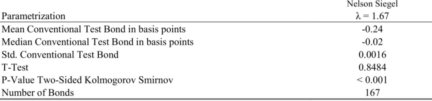
Nelson Siegel
Parametrization λ = 1.67
Mean Conventional Test Bond in basis points -0.24
Median Conventional Test Bond in basis points -0.02
Std. Conventional Test Bond 0.0016
T-Test 0.8484
P-Value Two-Sided Kolmogorov Smirnov < 0.001
Number of Bonds 167
Table 1 summarizes the results of our test procedure for the Nelson-Siegel specification. We run three different specifications, Siegel with flexible parameters, Siegel with constant parameters as suggested by Diebold and Li (2006) and Nelson-Siegel-Svensson parameters as suggested by Gilli, Große, and Schumann (2010).
The results of the parameter testing are summarized in Table 1. We find that the difference in-sample is not different from 0, according to the two-sided t-test. Additionally, we can reject the two-sided Kolmogorov Smirnov for the equality of the distribution between the subsample of test bonds and the computed ∆𝑦, of the green bonds to the 1% significance level. Both implicate that the fit of the Nelson-Siegel function is somehow accurate.
We proceed with specifications where 𝜆 =1.67 is fixed as suggested by Diebold and Li (2006) for two reasons. First, we find the average bond specific in-sample deviation from the market data is only -0.24bp and the median even smaller at -0.02bp, Second, the Svensson parameterization or other less restricted Nelson-Siegel parameterizations require larger computational resources. 𝛽 , 𝛽 and 𝛽 are restricted as suggested by Gilli, Große, and Schumann (2010).
For our sample of green bonds, 51,829 observations remain after eliminating the lowest and highest 5% percent. We recall that the yield gaps reflect the difference between the estimated yield for the green bond per the Nelson-Siegel curve and observed market data.
b. Stage 2: Fixed Effect Regression
In the second stage, we apply two different liquidity controls, ZTD and BAS and two different estimation methods, fixed effect with within heteroscedasticity and fixed effect with clustered heteroscedasticity and autocorrelation. To test whether we find autocorrelation and within cluster heteroscedasticity, we implement the following tests.
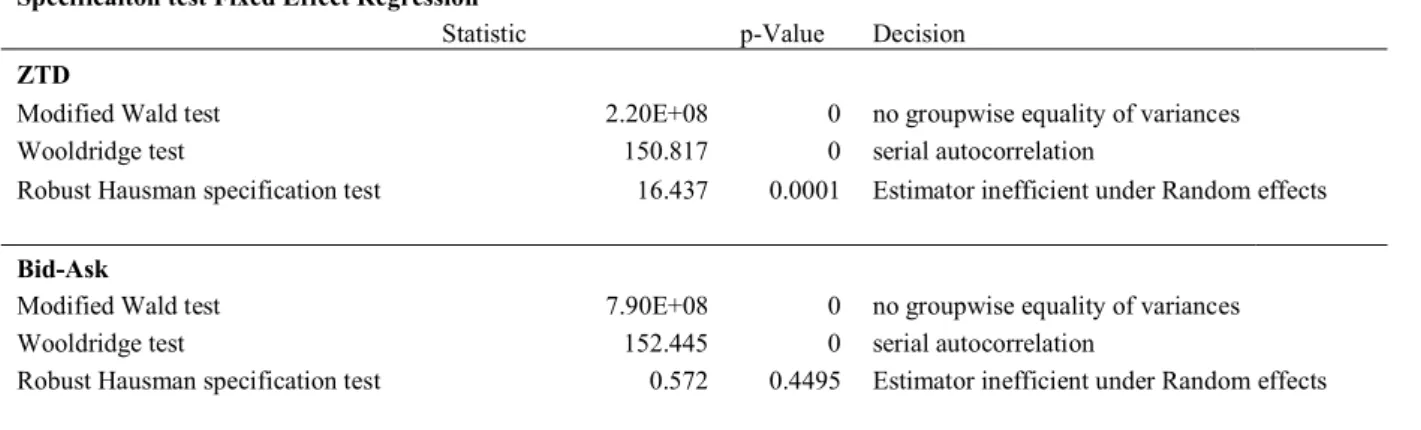
Specificaiton test Fixed Effect Regression
Statistic p-Value Decision
ZTD
Modified Wald test 2.20E+08 0 no groupwise equality of variances
Wooldridge test 150.817 0 serial autocorrelation
Robust Hausman specification test 16.437 0.0001 Estimator inefficient under Random effects
Bid-Ask
Modified Wald test 7.90E+08 0 no groupwise equality of variances
Wooldridge test 152.445 0 serial autocorrelation
Robust Hausman specification test 0.572 0.4495 Estimator inefficient under Random effects
Table 2 summarizes the results of the specification test we run to ensure that we establish the right fixed effect regression. We test for the efficiency of the fixed effect vs random effects with the robust Hausman test. The proxy ZTD is the difference between the number of period in the preceding 30 days, where the bond is not traded of the green bond and of the average of the conventional bond used to estimate the term structure of interest rates. The proxy BAS estimates the difference of the BAS spread of the green bond and the average of the conventional bonds used to estimate the yield curve.
The results of the test regression are summarized in Table 2. The Modified Wald tests for ZTD and for the BAS are rejected at the 1% significance level. Therefore, we can reject that the clustered variances are equal across the sample. The Wooldridge test for autocorrelation indicates that for the ZTD proxy and BAS we can reject the null at the 1% significance level as well. Thus, we do find autocorrelation in our sample and need to adjust the estimator accordingly.
We implement a Robust Hausman Test for Specification to decide whether fixed or random effect is the better fit for our model, to test whether our model accommodates for relationship between liquidity and premium. The results show that for the proxy ZTD the fixed effect with clustered standard errors is preferable to random effects with the same error term. This is not the case in the BAS regression. Therefore, we decide to proceed our analysis with the clustered estimator for within-heteroscedasticity, further only referred to as clustered, with the ZTD day indicator as a proxy for the difference in liquidity.
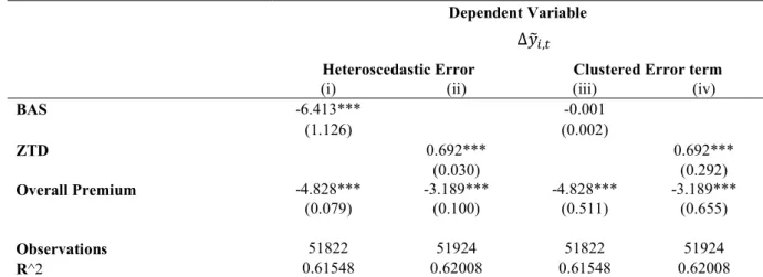
Dependent Variable
Heteroscedastic Error Clustered Error term
(i) (ii) (iii) (iv)
BAS -6.413*** -0.001 (1.126) (0.002) ZTD 0.692*** 0.692*** (0.030) (0.292) Overall Premium -4.828*** -3.189*** -4.828*** -3.189*** (0.079) (0.100) (0.511) (0.655) Observations 51822 51924 51822 51924 R^2 0.61548 0.62008 0.61548 0.62008
Table 3 summarizes the results of the fixed effect regression with the two liquidity proxies ZTD and BAS in basis points. Observation vary between the different models, because we drop observation, where we do not have market yields. The R^2 are reported as calculated in the regression with bond specific dummies. ‘*’, ‘**’, and ‘***’ denote values are significantly different from zero at 10%, 5%, and 1% respectively.
The estimation results from our fixed-effect regression are summarized in Table 3. We estimate BAS and ZTD with and without clustered error terms. The results for BAS suggest that an increase of 1bp in the difference in ZTD between the average of the conventional bonds and the green bond increases the premium by +0.692bp. Whereas the magnitude of the bid-ask spread dummy is small as well, the sign is the opposite and not significantly different from 0. However, we find that the size of the coefficient is relatively small in both cases.
The small impact of the liquidity variables might be driven by two effects. First, the screening of the bonds could filter large difference in liquidity. Second, the process of calculating the Nelson-Siegel curve could eliminate difference in liquidity, reducing the likelihood of being detected by the fixed effect regression.
In bps Min 1 Q Mean Median 3 Q Max Nr. Bonds Nr. of Days
ZTD -75.05 -15.54 -3.67 -1.86 8.47 72.82 160 51925
BAS -75.17 -15.84 -4.69 -2.53 8.37 72.08 160 51925
Table 4 summarizes the distribution of individual premiums in basis points estimated with ZTD and BAS accordingly. The choice of the error term structure, does not influence the estimation of the coefficient. 95.6% and 96,9% of the individual premiums are different from 0 at the 95% significance level, if the fixed income model is estimated with clustered error terms.
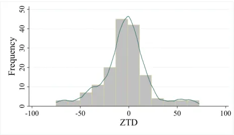
Figure 1 plots the bond specific premium results of ZTD with clustered error terms regression with the overlaid kernel density estimate in basis points. While the variance of the premiums seems high, the mean and median of the distribution are small, but negative. 0 10 20 30 40 50 Fr eq ue nc y 0 -100 -50 50 100 ZTD
Table 4 shows the estimated individual premiums. The mean of the estimation is -4bp and -5bp for the ZTD and BAS regression respectively. The premiums for the ZTD regression, after eliminating outliers, range between -74bp and +73bp, whereas 50% of the observations are in between -16bp and +8bp. The ZTD regression predicts that 60% of the individual premiums are negative. We note that the numbers of ZTD do not differ much from the BAS results. This can be used as an indication that both are subject to the above mention phenomena, the fact that the Nelson-Siegel eliminates larger differences in liquidity.
We test whether the bond specific premiums are significantly different than zero by implementing a constant-only regression. The computed test statistic, which can be found in the Appendix, suggests that the average bond specific premium using ZTD and BAS methodology respectively are different to 0 at the 10% and 5% significance level. From this evidence, we conclude that there is an indication about the existence of a 6small green bond premium. However, the high variance and the limited sample size of green bonds might misguide our conclusion. We proceed with the analysis of subsamples of the green bond estimates.
c. Stage 3: Determinants of the Green Bond Premium
As stated earlier, the researched sample is strongly heterogeneous. The sample includes different currencies, industrial and development markets as well as corporate and institutional issuers. Therefore, we aim to clarify the influence of geographical and sector specific factors on the estimated green bond premium. Additionally, we examine the development of the green bond premium on the size of the green bond premium.
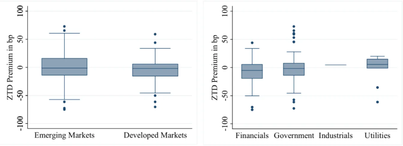
Figure 2 plots the distribution of green bond premiums by issuing market on the left side and by sector on the right side. We find that bonds issued in developed countries have a slightly higher
mean of green bond premiums than in emerging markets. The difference however is not significant as our test show.8
Figure 2 graphs the boxplot for the individual premiums sorted by currency. The boxplot indicates the upper adjacent value, 75% percentile, median, 25% and lower adjacent value. The markers indicate outside values.
The analysis regarding the sector does not provide us with further conclusion. Even though we find indication that financial issues receive with -7.25bp the highest premium, whereas governmental issuances, with 101 issues the biggest group, records a premium of -2.15bp, the differences are not significant. We conclude that within our sample, we do not find evidence that either the issuance markets or industries play an important role.
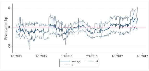
Additionally, we aim to analyze whether the green bond premium is constant over the observed period, or whether it changes significantly with time. Figure 2 plots the average difference in yield gap between January 2015 and May 2017 and the 95% confidence interval. The average yield gap9
8 Regression, which test for these determinants are found in the appendix. .
9 In this case, we ignore the liquidity impact. First, we may assume that the impact is constant over time. Second, we
assume that even if we estimate the premium without the liquidity, the size of the premium is somehow the same.
10 0 50 0 -5 0 -5 0 -1 00 -1 00 10 0 Z T D P re m iu m in b p
Emerging Markets Developed Markets
0 -1 00 50 -5 0 10 0 Z T D P re m iu m in b p
seems to have increased considerably within the last year. The estimated premium was smaller than 0 until the end of 2016, which is when it turned positive.
We can conclude that the premium is not constant over time. The regression result indicates that over the last 12 month the average premium increased from -17bp in the end of July 2016 to above +20bp in the end of our sample May 2017. Earlier issuances seem to have a higher premium than more recent recorded yields. After the expansion of the green bond market, this premium seems to diminish. A reason for this could be the declining difference in liquidity or the reduction of excess demand since supply increased strongly.
Figure 3 plots the average yield gap 𝑦 over our observed time-period. The black line indicates the average, whereas the dotted line plots the 95% confidence interval of the estimator. The lowest value -22.4bp is recorded in the beginning of Mid 2015 and the maximal value is recorded in end May 2017 with +26bp. The yield gap 𝑦 does not take in account the difference in liquidity.
V. Conclusion
This work introduces a method estimating the green bond premium. Instead of matching to the two closest bonds as Zerbib (2016), we extend this method and use up to twenty comparable bonds to
0 -5 0 50 P re m iu m in b p 1/1/2015 7/1/2015 1/1/2016 7/1/2016 1/1/2017 7/1/2017 average ul ll
estimate a term structure of interest rates, taking into consideration the different coupons paid on the conventional bonds. This implementation allows us to smooth through idiosyncratic yield variation and generate a price of a bond with the same characteristics and the same coupon as the green bond. This framework could be used in further research, which e.g. could use more elaborated measurements for liquidity to account for the difference in liquidity between the conventional and green bonds.
In our core estimation method, we find a green bond premium of -3.2bp. The estimated values are significantly different than 0, but smaller than prior research of Preclaw and Bakshi (2015) and Zerbib (2016) suggested. We conclude that investors trade green bonds on a slight premium. We find that leading up to the boom in issuances in 2016, our analysis indicates a larger negative premium up to -20bp at its maximum. We argue that this might be due to the excess demand in green bonds. After the supply of green bond increased, this premium seems to diminish as our estimates reach 0bp in the end of 2016 and turn positive in 2017.
We aim to support further quantitative and qualitative research in the field of green bonds, as we see a great potential in the bond market to finance the investment necessary to fight climate change. Future research may benefit from the larger available datasets to further understand the dynamics of the green bond pricing. An interesting question, which could be explored further, is whether the issuances of green bonds has beneficial impacts on all bonds of one issuer, instead of only the green bond itself.
Even though we do not find a strong premium, we conclude that green bonds have strong potential. We believe that with further development of market mechanism to ensure that the financed projects fulfill certain environmental standards, more extensive screenings and higher emphasis on external
valuation of included projects more standardization could be achieved. However, it should be taken into consideration that with more screening and valuation the benefits of the green bonds might outweigh the cost of diligence for the issuing company.
VI. References
Bauer, Rob and Daniel Hann. 2010. “Corporate environmental management and credit risk.” Available at SSRN 1660470.
BNEF. 2017. “Green Bonds: 2016 in Review. Research note.” Bloomberg New Energy Finance. Chava, Sudheer. 2014. “Environmental externalities and cost of capital.” Management Science,
60(9): 2223–47.
Diebold, Francis X. and Canlin Li. 2006. “Forecasting the term structure of government bond yields.” Journal of Econometrics, 130(2): 337–64.
Elton, Edwin J., Martin J. Gruber, Deepak Agrawal, and Christopher Mann. 2001. “Explaining the rate spread on corporate bonds.” The Journal of Finance, 56(1): 247–77. Fisher, Mark, Douglas W. Nychka, and David Zervos. 1995. “Fitting the term structure of
interest rates with smoothing splines.”
Gilli, Manfred, Stefan Große, and Enrico Schumann. 2010. “Calibrating the nelson-siegel-svensson model.”
Graham, Allan and John J. Maher. 2006. “Environmental liabilities, bond ratings, and bond yields.” Volume Advances in Environmental Accounting & Management, 3: 111–42. Graham, Allan, John J. Maher, and W. D. Northcut. 2001. “Environmental liability
Gürkaynak, Refet S., Brian Sack, and Jonathan H. Wright. 2007. “The US Treasury yield curve: 1961 to the present.” Journal of monetary Economics, 54(8): 2291–304.
ICMA. 2017. The Green Bond Principles 2017. Voluntary Process Guidelines for Issuing Green Bonds.
https://www.icmagroup.org/assets/documents/Regulatory/Green-Bonds/GreenBondsBrochure-JUNE2017.pdf (accessed August 6, 2017).
Longstaff, Francis A. and Eduardo S. Schwartz. 1995. “A simple approach to valuing risky fixed and floating rate debt.” The Journal of Finance, 50(3): 789–819.
McCulloch, J. H. 1975. “The Tax‐Adjusted Yield Curve.” The Journal of Finance, 30(3): 811– 30.
Nelson, Charles R. and Andrew F. Siegel. 1987. “Parsimonious modeling of yield curves.” Journal of business: 473–89.
Preclaw, Ryan and Anthony Bakshi. 2015. “The cost of being green.”
https://www.environmental-finance.com/assets/files/US_Credit_Focus_The_Cost_of_Being_Green.pdf.
Schneider, Thomas E. 2011. “Is environmental performance a determinant of bond pricing? Evidence from the US pulp and paper and chemical industries.” Contemporary Accounting Research, 28(5): 1537–61.
Sharfman, Mark P. and Chitru S. Fernando. 2008. “Environmental risk management and the cost of capital.” Strategic management journal, 29(6): 569–92.
Svensson, Lars E. O. 1994. “Estimating and interpreting forward interest rates: Sweden 1992-1994.” National Bureau of Economic Research.
VII. Annex
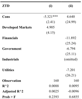
a. Green Bond Determinates
ZTD (i) (ii) Cons -5.321*** 4.640 (2.41) (24.99) Developed Markets 4.905 (4.15) Financials -11.892 (25.24) Government -6.794 (25.11) Industrials (omitted) Utilities -7.201 (26.21) Observation 160 160 R^2 0.0088 0.0095 Adjusted R^2 0.0025 -0.0096 Prob > F 0.2393 0.6855
Table 5 shows the regression resulting in the figure 2. ‘*’, ‘**’, and ‘***’ denote values are significantly different from zero at 10%, 5%, and 1% respectively.
b. Average Bond Specific Regression
ZTD BAS
Cons -4.695*** -3.666*
(1.89) (1.97)
Observation 160 160
Table 6 shows that the average of the bond specific constants are significantly different than 0. . ‘*’, ‘**’, and ‘***’ denote values are significantly different from zero at 10%, 5%, and 1% respectively.