DEPARTAMENTO DE FÍSICA
PROGRAMA DE PÓS-GRADUAÇÃO EM FÍSICA
DAVI SOARES DANTAS
EMERGENT VORTEX BEHAVIOR IN SUPERCONDUCTORS AND SUPERFLUIDS WITH SINGLE AND MULTICOMPONENT QUANTUM
CONDENSATES
EMERGENT VORTEX BEHAVIOR IN SUPERCONDUCTORS AND SUPERFLUIDS WITH SINGLE AND MULTICOMPONENT QUANTUM
CONDENSATES
PhD thesis presented to the Post-Graduation Course in Physics of the Federal University of Ceará as part of the requisites for obtaining the Degree of Doctor in Physics.
Advisor: Prof. Dr. Andrey Chaves.
Co-Advisor: Milorad V. Milošević.
Gerada automaticamente pelo módulo Catalog, mediante os dados fornecidos pelo(a) autor(a)
D211e Dantas, Davi Soares.
Emergent vortex behavior in superconductors and superfluids with single and multicomponent quantum condensates / Davi Soares Dantas. – 2017.
156 f. : il. color.
Tese (doutorado) – Universidade Federal do Ceará, Centro de Ciências, Programa de Pós-Graduação em Física , Fortaleza, 2017.
Orientação: Prof. Dr. Andrey Chaves. Coorientação: Prof. Dr. Milorad Milosevic.
1. Matéria de vórtice. 2. Interação vórtice-vórtice. 3. Supercondutores. 4. Condensados de Bose-Einstein. 5. Superfluidos. I. Título.
EMERGENT VORTEX BEHAVIOR IN SUPERCONDUCTORS AND SUPERFLUIDS WITH SINGLE AND MULTICOMPONENT QUANTUM CONDENSATES
Tese de Doutorado apresentada ao Programa de Pós-Graduação em Física do Departamento de Física da Universidade Federal do Ceará, como requisito parcial para obtenção do título de Doutor em Física. Área de concentração: Física da Matéria Condensada.
Aprovada em: 30/01/2017.
BANCA EXAMINADORA
_________________________________________________ Prof. Dr. Andrey Chaves (Orientador)
Universidade Federal do Ceará (UFC)
_________________________________________ Prof. Dr. Raimundo Nogueira da Costa Filho
Universidade Federal do Ceará (UFC)
_________________________________________ Prof. Dr. Carlos Alberto Santos de Almeida
Universidade Federal do Ceará (UFC)
_________________________________________ Prof. Dr. Milorad Milosevic
University of Antwerp
Science is never made alone. In fact, there is always a lot of social work behind every studied subject. Of course this was not different for me and therefore, there is a huge list of thanks. However, among all the people who supported me along this trajectory, it is easy to point out the one that was certainly the most important for the accomplishment of this work: my advisor, Andrey Chaves, who with patience and dedication gave me the background knowledge necessary for the conclusion of this thesis. Also, I will never forget the talks with Prof. Aristeu, which I had the pleasure of working with. Beyond their wise teachings on physics, I also consider them great friends of mine for their valuable time spent with me.
Standing over the shoulders of giants of science provided a shortcut for quality improvements of the work done in this thesis. For this reason, I will always feel indebted to my co-advisor, Prof. Milorad Milošević, who, with great wisdom and dedication, supported and taught me a lot along my doctorate and specially, during my staying in Belgium. In advance, I thank other members of the jury, Professors Clécio, Carlos Alberto and Raimundo, for the time spent reviewing this work, as well as for their very important comments, corrections and suggestions that made possible to improve the quality of the final version of this thesis.
In special, I warmly thank my friends of the undergraduate course at UFC and colleagues at GTMC and CMT research groups. Last but not least, I thank to my family: my mother, Lucia, my brother, Bruno and my wife Lorrayne for always being present in difficult moments that I passed by. Finally, I thank my father, who unfortunately could not witness this moment of achievement, but who would certainly be very proud of it.
Using a self-devised numerical approach, we developed a powerful tool to investigate vortex properties and interactions in mean-field theories for superconductors and superfluids, based on fixing the vortex phase distribution in the energy minimization process. The method was applied to (i) multi-component Bose-Einstein condensates (BECs) and (ii) superconductors with single- or multi-component superconducting condensates. In these systems, vortex-vortex interaction and other key vortex features are analytically described only in specific regimes, that do not account for a large part of vortex behavior observed experimentally. In multi-component BECs, for example, the vortex-vortex interaction is only known for inter-vortex distances much greater than the healing length, i.e. far from the vortex core. Under our approach, by assuming multi-vortex structures, within Gross-Pitaevskii theory, we report the vortex-vortex interaction in the full range of distances, capturing the mechanism behind unusual vortex conformations previously reported in literature, such as bound clusters with two or three vortices. Usually, these clusters emerge from a competition between intra- and inter-component vortex interaction, but we demonstrate they can also emerge from the phase-frustration between the components.
In superconductors, the description of vortex-vortex interaction is usually restricted to bulk or very thin films, and most of the key vortex features, such as the spatial magnetic field and current density profiles, are known only in the limit of London theory, i.e. for coherence length ξ negligible as compared to magnetic field penetration depthλ and other system dimensions. The parametric range outside this limit is actually relevant to many materials. We fill that gap by applying our method to Ginzburg-Landau theory. The vortex structure is investigated for single- and two-gap bulk superconductors, outside the London regime. This enables us to extend analytical expressions describing the condensate and magnetic profiles around the vortex available in literature by numerical calculations and suitable fitting functions. We expand our approach to account for films with finite thickness, to connect our findings to both bulk and Pearl’s description by adjusting the sample thickness. This also allowed us to describe how vortex configurations change for samples with intermediate thickness, where we observe the effective magnetic response of the superconductor changing between the textbook type-1 and type-2 behaviors, in a nontrivial manner, governed by the non-monotonic vortex interaction. As a result of a detailed analysis, we propose new critical parameters to define the crossover between different regimes and establish their relation with the superconducting critical fields.
Keywords: Vortex matter. Vortex-vortex interaction. Superconductors. Bose-Einstein
Usando uma abordagem numérica própria, desenvolvemos uma ferramenta poderosa para investigar propriedades e interações de vórtices na teoria do campo médio para supercondutores e superfluidos, baseada na fixação da distribuição de fase dos vórtices no processo de minimização da energia. O método foi aplicado a (i) condensados de Bose-Einstein (BECs) com múltiplas componentes e (ii) supercondutores com um ou mais condensados que super-conduzem. Nesses sistemas, a interação vórtice-vórtice e outras características chaves são analiticamente descritas apenas em regimes específicos, que não descrevem grande parte do comportamento dos vórtices observados experimentalmente. Em condensados de Bose-Einstein com múltiplas componentes, por exemplo, a interação vórtice-vórtice é conhecida apenas para distâncias muito maiores que o comprimento de coerência, i.e. longe do centro do vórtice. Sob nossa abordagem, assumindo estruturas com múltiplos vórtices, dentro da teoria de Gross-Pitaevskii, nós reportamos a interação entre vórtices em todo o domínio de distâncias, capturando o mecanismo por trás de conformações de vórtices não usuais previamente reportadas na literatura, como aglomerados ligados com dois ou três vórtices. Sabe-se que, geralmente, esses aglomerados emergem da competição entre interações de vórtices intra-componentes com interações inter-componentes, no entanto, nós demonstramos que essas também podem emergir da frustração de fase entre as componentes.
Palavras-chave: Matéria de vórtice. Interação vórtice-vórtice. Supercondutores.
Figure 1 – Classical and quantum regimes in the temperature-density plane. The rough dividing line isnλ3
T = 1, where λT is the thermal wavelength and n stands for the density of particles. . . 26 Figure 2 – The mean occupation number hnǫi of a single-particle energy state ǫ
in a system of non-interacting particles for Fermions (red line), Bosons (blue line) and classical particles (yellow line). Acronyms F.D., M.B. andB.E. respectively account for the Fermi-Dirac, Maxwell-Boltzmann and Bose-Einstein distributions governing particle’s statistics. . . 29 Figure 3 – Function g3/2 as a function of the gas fugacity represented by the blue
line. The yellow line show that g3/2 can be approximated by a linear function for low values of z. . . 30 Figure 4 – Phase diagram of Bose-Einstein condensation in the density-temperature
plane. . . 31 Figure 5 – Observation of Bose-Einstein condensation by means of absorption
imaging technique, where the absorption is illustrated as a function two spatial directions for temperatures above, just below and well below the critical temperature, respectively illustrated in pictures from the left-to right-hand side. Figure retrieved from Ref. (DURFEE; KETTERLE, 1998). . . 33 Figure 6 – Sketch of a normal fluid and a superfluid in a rotating vessel. Whereas
normal fluids experiment a rigid-body rotation, superfluids rotate by forming arrays of quantized vortices. . . 43 Figure 7 – Miscible and Imiscible conditions in the inter-particle interactions phase
diagram. . . 47 Figure 8 – Sketch of the phase diagram of an arbitrary superconducting material.
The superconducting phase is delimited by the critical values of current ~j, magnetic field H~ and temperature T. From a practical point of view, these critical values are in general very small, making it difficult for commercial applications. . . 48 Figure 9 – The electrical resistance of mercury as a function of temperature. Here,
Figure 11 – The expected experimental outcome from the perfect conductance the-ory: (a) The superconducting material is firstly subjected to an external magnetic field and then cooled down below its critical temperature, "freezing" the magnetic field inside the sample; and (b) The material is first cooled down below Tc and then, an external magnetic field is ap-plied. Since ˙B~ = 0, the magnetic field inside the sample should remains null. . . 52 Figure 12 – Magnetization as a function of the applied field for: (a) a type-I
super-condunctor and (b) a type-II superconductor. . . 54 Figure 13 – A singly connected surface S under and externally applied magnetic
field H~. . . 56 Figure 14 – Kinetic energy of superconducting electrons in a hollow cylinder as a
function of magnetic flux. . . 57 Figure 15 – The free energy density difference between superconducting and normal
states Fs0−Fn0 as a function of Ψ forβ = 1.0 and three different values of α: -1.0 (blue triangles), 0.0 (yellow squares) and 1.0 (red circles). . . 58 Figure 16 – The superconducting/normal metal interface: the illustration of the
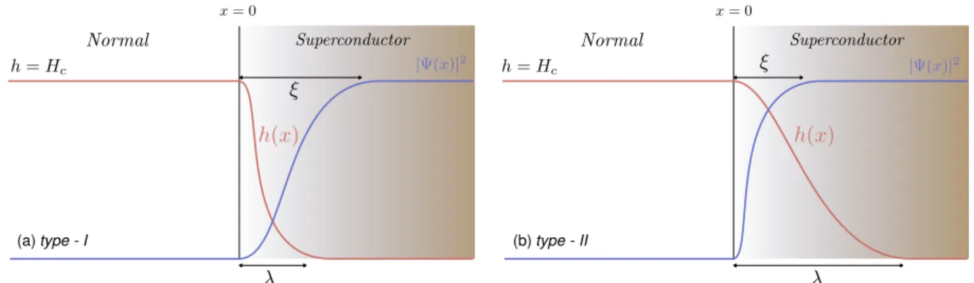
spatial dependence of the superconducting order parameter|Ψ|where b denotes the extrapolation length. . . 62 Figure 17 – Magnetization as a function of the applied field for: (a) a type-I
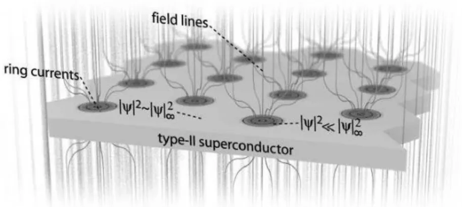
super-condunctor and (b) a type-II superconductor. . . 66 Figure 18 – Sketch of quantized vortices in a type-II superconducting sample. Figure
retrieved from Ref. (MOSHCHALKOV; FRITZSCHE, 2011). . . 67 Figure 19 – First image of Abrikosov vortex lattice in a dopped Pb sample using
Bitter decoration. Figure retrieved from Ref. (ESSMANN; TRÄUBLE, 1967). . . 68 Figure 20 – Mechanism behind electronic attraction in an ion lattice. Due to the
polarization cloud left by an electron traveling through the ion lattice, a second electron may experience a net attractive interaction. Figure made by the author, based on a Wikipedia image. . . 68 Figure 21 – Stirred Bose-Einstein condensation before vortex entry in panels (a)
and (c). First vortex observation image after exceed the critical rotation frequency in (b) and (d). This figure was retrieved from Ref. (MADISON et al., 2000a). . . 78 Figure 22 – Observation of Abrikosov vortex lattices in a stirred Bose-Einstein
Ref. (KUOPANPORTTI; HUHTAMÄKI; MÖTTÖNEN, 2012) . . . . 80 Figure 24 – Triangular conformation of vortex molecules obtained in coherently
coupled three-component Bose-Einstein condensate. Figure retrieved from Ref. (ETO; NITTA, 2012) . . . 81 Figure 25 – Vortex-vortex interaction potentials, considering M12 = 2.0, for
(a-b) two vortices in the same component and (c) vortices in different components. Colours and symbols denote different inter-component coupling strength: γ12 = −0.20 (blue circles); γ12 = −0.45 (yellow squares);γ12= −0.75 (red triangles); andγ12 =−0.98 (green downward triangles). . . 85 Figure 26 – The occupation number density contour plots for: (a) first component
with two vortices positioned at (−d/2,0) and (d/2,0) and (b) second component with a single vortex in the center of the mesh. Notice the depleted density in one component in the positions where the other component features a vortex. The investigation of the system energy with respect tod for this conformation enables us to identify possible bound states in a two-component Bose-Einstein condensate with mass ratio M12 = 2.0. . . 86 Figure 27 – (a) Total energy for three vortices configuration U21, characterizing a
binary system with M12 = 2. The vortex in the second component is fixed in the center of the mesh, whereas vortices in the first component are placed at symmetric positions separated by distanced. (b) A mag-nification of the particular case γ12=-0.98 shows that in the favored configuration, the two vortices in the first component are located on top of each other, and on top of the vortex in the second component. (c-f) Occupation number density of both components, considering vortices separated by 100 ξ, for all cases considered in (a), where the solid (dashed) line stands for the first (second) component. . . 87 Figure 28 – (a) Total energy of a three vortex structure in a two-component BEC,
forγ12=−0.90 (blue circles) and−0.92 (red squares). The curve bumps may lead to non-triangular lattices, despite the overall repulsive behavior. (b) Particular case of a triple-vortex structure with γ12=−0.95. The
minimum far from the origin allows for the formation of dimers for specific vortex densities. (c) Dimer configuration profile for γ12 =−0.95. 88 Figure 29 – Vortex core size as a function of the inter-component coupling, for
values of γ12. . . 90 Figure 31 – The occupation number density contour plots of: (a) first component
with a vortex positioned at (0,√3d/4); (b) second component with a vortex positioned at (−d/2,−√3d/4) and ; (c) third component with a vortex positioned at (d/2,−√3d/4). . . 91 Figure 32 – (a) Total energy U111, for the equilateral triangle vortex configuration
as a function of the side d for γ = 0.45 and for several values ofω. (b) Plot of the optimal side of the equilateral vortex triangle against ω for γ = 0.45. The red line represents a power law with exponent −0.3214 and coefficient 0.9265. (c) Same as (b) but for γ = 0.60. The red line represents a power law with exponent −0.3186 and coefficient 1.0746. . 92 Figure 33 – (a) Total energy U111 as a function of the displacement of the first
component vortex xv1 from S1 position in the x direction. (b) Total energy U111 as a function of the displacement of the first component vortex yv1 from the origin in the y direction. For both cases, we have considered γ = 0.45 and ω = 1.7× 10⁻⁴. The vertical dashed line represents the coordinates of first component vortex for the minimum energy equilateral triangle configuration. . . 93 Figure 34 – (a) Total energy U111, with vortices of the first and second components
pinned in the center of the mesh, as a function of the third component vortex distance d from the origin, for different values of the third component extra phaseφ3: 0 (solid blue line),π/6 (green dashed dotted line), π/3 (yellow dashed line) and π/2 (red dotted line), with ω12 = ω13 =−ω23= 1×10⁻². (b) Total energyU111 for the same conformation of (a), keeping φ3 = 0 and assuming different values of ω:ω = 1×10⁻² (blue circles),ω = 2×10⁻² (green squares),ω = 3×10⁻² (yellow upward
triangles) andω = 4×10⁻² (red downward triangles). . . 94 Figure 35 – (a) Sketch of the circulating current density distribution around the
(blue solid line), 2.0 (green dotted-dashed line), 4.0 (yellow dashed line) and 8.0 (red dashed-dashed-dotted line). (c) Vortex and magnetic core represented by gray circles and red squares respectively. The vertical black dashed line represents the transition point κc = 1/
√
2 between type-I and type-II regimes. . . 106 Figure 37 – (a) Angular current density for different κ values: 0.4 (blue solid line),
0.6 (green dotted-dashed line), 0.8 yellow (dashed line) and 1.0 (red dotted-dashed-dashed line). (b) Peak position of angular density current (red circles) as a function of κ, within an appropriate fitting function (solid gray line). (c) Magnetic field in vortex center as a function ofκ. For κ= 1/√2, the magnetic field in the vortex center is exactlyH(0) = 1Hc, which is the magnetic signature of type-I/type-II transition in single-band bulk superconductors. . . 107 Figure 38 – Magnetic field difference at vortex core between double and single vortex
conformations as a function of the inter-vortex distance d for different values of κ: 0.4 (black circles), 0.5 (red squares), 0.6 (green triangles), 0.7 (blue diamonds), 0.8 (yellow downward triangles), and 1.0 (pink rightward triangles). . . 108 Figure 39 – Vortex profile in a superconducting bulk for different values of
Ginzburg-Landau parameter κ: 0.2 (blue circles), 0.8 (yellow squares), 4.0 (yellow dashed line) and 8.0 (red triangles) and their respective fittings repre-sented by dashed lines . The inset provide the fitting parameter ν as a function of the Ginzburg-Landau parameter κ. . . 109 Figure 40 – (a-c) Magnetic profiles for superconducting bulk samples, with different
values of Ginzburg-Landau parameter κ: 2.0, 4.0 and 8.0 respectively. Red dashed lines represent fittings made from r ≥λ up to 80ξ using the function µ. Fitting parameters µ> and µ< as a function of the Ginzburg-Landau parameter in panels (d) and (e), respectively. . . 110 Figure 41 – The parameter µ0 as a function of κ is represented by blue squares,
whereas the gray dashed line stands for the fitting functionα+βκ−1, with α= 1.28 and β = 1.73 . . . 111 Figure 42 – Cooper pair density, angular current density and transverse component
dotted-dashed line), 2.0 (yellow dashed line) and 8.0 ( red dotted-dashed-dashed line). (c-d) Vortex and magnetic core radius as a function of thickness sizeδ for four different values ofκ: 0.4 (solid line), 0.6 (dashed line), 0.8 (dotted-dashed line) and 1.0 (dotted-dashed-dashed line). The corresponding horizontal red lines stand for asymptotic behavior of each curve, which was obtained through the bulk case solution. . . 113 Figure 44 – (a) Cooper pairs density for κ = 0.4 and different values of thickness
δ: 0.2 ( blue circles), 1.0 (yellow squares) and 12.0 (red triangles). Dashed lines stand for the corresponding fitting functions. (b) The fitting parameter ν as a function of the sample thickness δ for different values of Ginzburg-Landau parameter κ: 0.4 (solid line), 0.6 (dashed line) and 0.8 (dotted-dashed line). . . 114 Figure 45 – Long-range magnetic profile for κ= 1.0 and different values of sample
thickness δ: 0.20, 0.25, 1.0 and 2.0 respectively illustrated by circles in panels (a-d). Here, solid lines account for fitting functions that resembles Pearl’s prediction for the magnetic field. . . 115 Figure 46 – (a-c) Magnetic profiles and their corresponding fitting functions
re-spectively illustrated for three different values of κ = 0.6 , 0.8 and 1.0. Three different values of sample thickness δ are considered in each panel: 1.0 (circles), 2.0 (squares) and 8.0 (triangles). Short(long)-range fitting functions are expressed by blue(red) solid(dashed) lines. (d-g) Fitting parameters are plotted as a function of sample thickness for three different values of κ: 0.6 (plus symbol), 0.8 (x symbol) and 1.0 (stars). . . 116 Figure 47 – Average transverse component of the magnetic field peak and the peak
position of the angular density current as a function of sample thickness δ for different values of Ginzburg-Landau parameterκ: 0.4 (blue circles), 0.6 (green squares), 0.8 (yellow upward triangles) and 1.0 (red downward triangles) respectively illustrated in panels (a) and (b). Solid lines account for the fitting functions expressed in Eqs. 3.25 and 3.26 with parameters of Table 1. . . 117 Figure 48 – (a) Single and multi-quanta vortex profiles for δ = 2.0 and κ =
thickness were assumed: δ= 1.0 (blue solid line), δ= 2.0 (green dotted-dashed line), 4.0 (yellow dotted-dashed line) and 8.0 (dotted-dotted-dashed-dotted-dashed line). . . 119 Figure 50 – Stability test of giant-vortex states with n = 2,3 and 4 respectively
illustrated in panels (a), (b) and (c) for different values of thickness δ: δ = 1.0 (blue solid line),δ = 2.0 (green dotted-dashed line), 4.0 (yellow dashed line) and 8.0 (dotted-dashed-dashed line). . . 120 Figure 51 – (a) Magnetic profiles of giant-vortices (n = 3) forδ = 2.0ξ and different
values ofκ: 0.30 (blue solid lines), 0.35(yellow dashed-lines), 0.40 (red dashed-dotted lines). (b) Corresponding stability tests through the giant-vortex-vortex interaction calculation . . . 121 Figure 52 – Perpendicular component of magnetic field profile alongz direction with
vorticities n= 1,2,3 and 4 in panels (a-d), respectively. In each panel, three different sample thickness δ were consideredδ= 1.0,2.0 and 4.0ξ 121 Figure 53 – Vortex profiles of σ- and π- bands respectively exhibited in panels (a)
and (b) for a MgB2-like material with different values of the σ-band Ginzburg-Landau parameter κ1: 1.0 (blue solid line), 4.0 (red dotted-dashed line) and 8.0 (yellow dotted-dashed line) . The corresponding magnetic field profiles in (c). (d) The vortex and magnetic core radius as a function of κ1 parameter in (d), where the vortex core of σ and π bands are respectively designed by black circles and gray squares, whereas red triangles stands for the magnetic field core. . . 122 Figure 54 – Vortex-vortex interaction near transtion points. In panel (a) and (b),
the transtions attractive/non-monotonic and non-monotonic/repulsive are respectively investigated by assuming different values of κ1: 3.0 (blue circles), 4.0 (red squares), 6.0 (gray losangles), 8.0 (yellow upward triangles), 10.0 (violet downward triangles) and 14.0 (green rightward triangles). . . 123 Figure 55 – Vortex profiles of σ- and π- bands respectively exhibited in panels (a)
thickness δ = 4ξ and κ= 0.4. Inner (outter) surfaces represent regions with higher (lower) magnetic field. (b) Magnetic field profile along the z−direction, calculated in one of the vortex cores, for film thickness δ = 1 (blue solid line), 2 (yellow dashed line) and 4 ξ (red dotted-dashed line). The film limits in z in each case are illustrated by vertical lines. . 127 Figure 57 – Vortex-vortex interaction potential as a function of the vortex separation
for δ = 1.0 and different Ginzburg-Landau parameterκ in (a) and for κ= 0.4 and different film thicknessδin (b). In (c) Interaction potentials between a giant-vortices and vortices with vorticitiesn1 and n2 in the κ = 0.3 and δ = 1.0ξ case. The n1 = n2 = 1 case is shown again for comparison with the cases with different vorticities. . . 128 Figure 58 – Randomly nucleated giant vortices at 6.9 K after ZFC and then
pro-gressively increasing the magnetic field to (b) 10.3 Oe and (c) 10.5 Oe. (d) SHPM image taken after shaking the vortex pattern of (c) with
hac = 0.1 Oe for 30 s. This figure was retrieved from Ref. (GE et al., 2013). . . 129 Figure 59 – (a) κ vs. δ phase diagram illustrating different types of regimes in
superconducting films: II (red), giant-vortex state (gray) and type-I (blue). The black dashed line indicates whether the giant-vortex with n = 2 represents the ground state or not. (b) Redefined critical Ginzburg-Landau parameter (black circles), along with its corresponding fitting functions in both thin (red dashed line) and thick (blue solid line) limits, with α= 0.36,β = 0.39,γ = 0.57 and ζ = 1.07. . . 130 Figure 60 – (a) κ vs. δ phase diagram showing attractive (blue background) and
repulsive (red background) interaction regimes according to the energetic contribution inside the sample and (b) dividing line between both regimes with its correponding fitting function α√δ, for α= 0.54 (black solid line) and the expected coefficient α= 0.59 (orange dashed line). . 131 Figure 61 – (a) Energy difference between superconducting and normal domains as
squares) and 0.5 (red triangles); and their corresponding asymptotic values (dotted lines). Fitting functions Hc/Hc2 = ακ[1 −
q
(βκ/δ)] are represented by dashed lines, with fitting parameters (α0.3, β0.3) = (0.22,0.47), (α0.4, β0.4) = (1.71,0.38) and (α0.5, β0.5) = (1.38,0.24). (b)
Critical field near the film limit for κ= 0.5. Red and gray backgrounds account for the short-range repulsion and short-range attractive regimes. 133 Figure 63 – (a) Dividing line between short-range attractive and short-range
1 INTRODUCTION . . . . 25
1.1 Introduction to Bose-Einstein Condensates . . . 25
1.1.1 Thermal wavelength and quantum effects . . . 26
1.1.2 Ideal Bose gas . . . 27
1.1.2.1 Bose-Einstein distribution . . . 27
1.1.2.2 BEC in an ideal gas . . . 29
1.1.3 Path towards BECs . . . 32
1.1.4 Theoretical description of an interacting Bose gas . . . 35
1.1.4.1 Second quantization and the many-body Hamiltonian . . . 35
1.1.4.2 Bogoliubov approach . . . 39
1.1.4.3 Landau superfluidity criterion . . . 41
1.1.4.4 Vortex states . . . 42
1.1.4.5 The Gross-Pitaevskii equation . . . 44
1.1.4.6 Time-independent GPE . . . 45
1.1.4.7 GPE for two-component BECs . . . 46
1.2 Introduction to superconductivity . . . 48
1.2.1 Experimental background . . . 50
1.2.1.1 Meissner Effect . . . 52
1.2.1.2 Type-I and Type-II superconductivity . . . 53
1.2.2 London’s description . . . 54
1.2.2.1 Flux quantization . . . 56
1.2.3 The Ginzburg-Landau theory . . . 58
1.2.3.1 Boundary conditions . . . 61
1.2.3.2 Characteristic length scales . . . 63
1.2.3.3 Superconducting types according to GL theory . . . 64
1.2.4 Vortex states and Abrikosov flux lattice . . . 66
1.2.5 BCS theory . . . 68
1.2.5.1 Revisiting the non-interacting Fermi-gas atT = 0 . . . 69
1.2.5.2 Cooper pairs . . . 69
1.2.5.3 The BCS theory . . . 72
TICES IN MULTI-COMPONENT BECS: THE ROLE OF THE
VORTEX-VORTEX INTERACTION . . . . 76
2.1 Introduction . . . 76
2.2 Vortex states in BECs . . . 78
2.2.1 Single-component BECs . . . 78
2.2.2 Multi-component BECs . . . 80
2.3 Our theoretical approach . . . 81
2.4 Numerical Results . . . 84
2.4.1 Two-component BEC with contact interaction . . . 84
2.4.2 Vortex dimers and trimers in coherently coupled BECs . . . 90
II
SUPERCONDUCTORS
96
3 VORTEX CHARACTERIZATION IN SINGLE- AND TWO-GAP SUPERCONDUCTING BULK AND FILMS . . . . 973.1 Introduction . . . 97
3.2 Vortex structure . . . 99
3.2.1 On bulk samples . . . 99
3.2.1.1 Magnetic structure . . . 99
3.2.1.2 Cooper pairs . . . 100
3.2.2 On films . . . 101
3.3 Theoretical Model . . . 103
3.3.1 Double-gap superconductors . . . 104
3.4 Results . . . 105
3.4.1 Bulk . . . 105
3.4.2 Films . . . 111
3.4.2.1 Singly-quantized vortices . . . 111
3.4.2.2 Multi-quantized vortices . . . 118
3.4.3 Double-gap bulk superconductors . . . 122
4 NON-MONOTONIC VORTEX-VORTEX INTERACTIONS AT THE TYPE-I TO TYPE-II TRANSITION OF THIN SUPER-CONDUCTING FILMS. . . . 125
4.1 Introduction . . . 125
4.2 Results . . . 126
1 Introduction
In what follows, we present a brief introduction to both Bose-Einstein con-densation and superconductivity theories in order to bridge the gap between fundamental concepts and the current research presented in this thesis. Unfortunately, summarizing over a hundred years of research in just a single chapter within the didactic purpose of teaching is certainly not a conceivable task and lies outside the scope of this thesis. There-fore, only topics directly related to the research presented in this thesis will be carefully reviewed in this thesis. In this chapter, we shall make a brief return to the past, in order to provide an historical perspective of the progress made in both fields. Starting from their prediction/discovery, some of relevant achievements which contributed substantially to the condensed state description are briefly revisited. Whenever necessary, a deeper review may be presented in subsequent chapters.
1.1 Introduction to Bose-Einstein Condensates
matter to be exhibited in large scales (KETTERLE, 2007; PETHICK; SMITH, 2002). This collective behavior paved the way towards the discovery of a new state of matter usually masked by thermal motion of system particles, named Bose-Einstein condensation (BEC) in honor of its discoverers Satyendra Nath Bose and Albert Einstein. In this new state, the gas behaves as a superfluid, (FETTER, 2009a; DALFOVO et al., 1999) experiencing no flow resistance and, therefore, it no longer obeys the classical hydrodynamics description.
1.1.1 Thermal wavelength and quantum effects
Quantum effects arising from the wave nature of particles manifest themselves macroscopically only under very restricted conditions of density and temperature. To a first approximation, the critical temperature Tc might be derived as the emerging point of an identity crisis, where the spatial extension of wave packets associated with gas atoms becomes of the order of the inter-atom distances. According to the de Broglie conjecture (BROGLIE, 1924), the spatial extension of these wave-packets is governed by the de Broglie wavelength hλi=h/hpi, where hpi is the average momentum of particles in the gas. The wavelength is, therefore, closely related to the thermal motion of the system. At equilibrium, the energy equipartition law holds,
hpi2 2m =
3
2kBT, (1.1)
and the spatial extension of wave packets can be defined in terms of the gas temperature T, leading to the thermal wavelength definition λT = h/√3mkT. Because the average inter-particle distance is of the order of n1/3, where n is the gas density, the quantum regime emerge when the phase space density, D ≡ nλ3
T, approaches unity. A sketch of the phase transition is illustrated in Fig. 1, where quantum and classical regimes are respectively represented by the blue and red backgrounds.
n
T
Classical
Regime nλ
3=1
Quantum Regime
Figure 1 – Classical and quantum regimes in the temperature-density plane. The rough dividing line is nλ3
T = 1, where λT is the thermal wavelength andn stands for the density of particles.
In this regime, particles in a gas might be treated as billiard balls, obeying the Maxwell-Boltzman statistic (HUANG, 1963). On the other hand, whenever the temperature of a non-interacting gas becomes low enough and the density high enough such that the phase space density approaches unity, the quantum indistiguishability of system particles becomes relevant and must be taken into account in the theoretical description. Usually, the indistinguishability is expressed in quantum theory by imposing symmetry constraints on the state functions and on the observables, bringing consequences which deeply affect the physical nature of the system (LEINAAS; MYRHEIM, 1977). These constraints emerge from the invariance of measurable physical quantities with respect to a particle permutation. From the statistical point of view, the main difference between both regimes is the way that we count the number of different system states. Indeed, in the classical formalism, each identical system particle is treated as distinguishable, which implies that the permuting between any two identical particles of the system leads to different states. On the other hand, in the quantum mechanics description, this is no longer valid and a symmetry (anti-symmetry) between the N! permutations of bosonic (fermionic) particles appears for the same physical state. This redundancy, called exchange degeneracy, violates the state vector unicity for each physical state and then must be eliminated from the theoretical formalism by limiting the state vector space to a subspace that is invariant under the permutation of labels (SAKURAI; NAPOLITANO, 2011).
1.1.2 Ideal Bose gas
To statistically address elementary effects derived from the indistinguishability of quantum particles, Einstein firstly expanded upon Bose’s suggestion to a gas of N non-interacting quantum particles confined in a volume V and sharing a certain amount of energy E. Within their approach, named Bose-Einstein statistics, they predicted the novel state of matter by making no reference at all to the interaction between gas atoms. It is worth to mention that, at the time of Bose-Einstein condensation prediction, in 1924, some of the basic concepts of quantum mechanics were not yet discovered. For instance, strange as it may seem, the uncertainty principle of Heisenberg was derived only three years later. Actually, as pointed out in Ref. (DELBRUCK, 1980), the Bose-Einstein statistics may have arisen from an elementary “mistake" of Bose, which was subsequently reproduced by Einstein. The deep meaning of Bose’s assumptions could only be understood after the working out of quantum mechanics (DELBRUCK, 1980). In this section, the statistical prediction of Bose-Einstein condensation is briefly reviewed, but without going into further details on the cumbersome historical path.
1.1.2.1 Bose-Einstein distribution
along the system energy spectrum under macro-state constraints (N, V, E). From the principle of equal a priori probabilities, the distribution with the largest number of micro-states is more likely to occur and therefore should represent the system ground state (REIF, 1965). This requires the knowledge of the number of micro-states Ω(N, V, E), for each possible distribution. In the thermodynamic limit, where fluctuations around the average are negligible, the system total energy spectrum should be regarded as a continuum (PATHRIA, 1995; HUANG, 1963; REIF, 1965; ANNETT, 2004). Therefore, in order to to count accessible states, the energy spectrum might be divided into a large number of energy cells, indexed by k = 1,2,3.... Let ǫk denote the average energy of cellk and gk the number of states inside it. Each cell contain a large, but still arbitrary, number of states, which means that gk >> 1. Thus, the problem consists in finding how many different ways one can group n1 particles in the first cell, n2 particles in the second cell and so on, following the macro-state constraints of number of particles and total energy,
X
k
nk =N, (1.2a)
X
k
ǫknk =E. (1.2b)
Because exchanging of particles in different cells does not produce a new different state, the number of distinct microstates associated with each cell, w(k), may be calculated separately, as the number of ways to accommodatenk particles amonggk levels. The total number of microstates, Ω(N, V, E), associated with the set {nk}, results from
Ω(N, V, E) = Y
k
w(k), (1.3)
where, for bosons,w(k) can be achieved by counting the number of arrangements between nk balls and gk−1 walls separating energy cells, which is given by
w(k) = (nk+gk−1)!
nk!(gk−1)! . (1.4)
In the thermal equilibrium, the particles might distribute themselves such that the entropy S is maximized. Thus, the distribution of bosons may be obtained by maximizing the function S = kBlnΩ, where kB is the Boltzmann constant. Through straightforward calculations, the result first obtained by Bose and Einstein is found
nk = gk
e(ǫk−µ)/kBT −1, (1.5)
where µ is the chemical potential and T the temperature (HUANG, 1963; PATHRIA, 1995; ANNETT, 2004). Roughly, the Bose-Einstein distribution is the most random way to distribute particles among system’s micro-states under the constraints of fixed number of particles N and total energyE (INGUSCIO et al., 1999). The average number of particles occupying any single quantum state is given by the ratio ni/gi,
hnki= 1
1.1.2.2 BEC in an ideal gas
Unlike the classical ideal gas, or the Fermi-Dirac gas, the Bose-Einstein gas presents a very peculiar regime. In fact, as illustrated in Fig. 2, if the chemical potential µ becomes equal to the energy level ǫk, the average number of particles of thek-th states becomes infinitely high. The condensation of particles in a single state, however, can only occur for the lowest energy level, otherwise the occupation number of some states would assume negative values, which has no physical meaning. This macroscopic occupation of the lower energy state is reflected in the abrupt changes on thermodynamical properties, signed by a change of behavior in specific heat that closely resembles theλ-point transition observed in liquid helium (FEYNMAN, 1957).
-3 -2 -1 0 1 2 3
(ε
i-
µ)/
k
BT
0.0 1.0 2.0
<n
i
>
B. E.
M. B.
F. D.
Figure 2 – The mean occupation number hnǫi of a single-particle energy stateǫ in a sys-tem of non-interacting particles for Fermions (red line), Bosons (blue line) and classical particles (yellow line). AcronymsF.D.,M.B.andB.E.respectively ac-count for the Fermi-Dirac, Maxwell-Boltzmann and Bose-Einstein distributions governing particle’s statistics.
Making the chemical potential approach the ground state energy is probably the simplest way to observe the origin of Bose-Einstein condensation phenomenon. However, it is by no means something rigorous, since it provides no clue on the fraction of condensed particles or even the critical temperature required to define this new state of matter. The comprehensiveness of phase transition’s thresholds lies somehow on the total number of particles constraint and emerges as a pathology derived from the inability to count for ground-state particles in thermodynamic limit. In the thermodynamic limit, the sum over discrete quantum states of Eq. (1.2a) might be replaced by an integral over the continuum energy spectrum and the density of particles may be written
n =
Z ∞
0
g(ǫ)
e(ǫ−µ)/kBT −1dǫ, (1.7)
density of states becomes
g(ǫ) = m 3/2
√
2π2¯h3ǫ
1/2. (1.8)
Here, it is worth mentioning that, symmetry properties of particles are not included in the density of states. In fact, their quantum nature is completely contained on Bose-Einstein distribution, that governs allocation of particles among micro-states. The outcome of Eq. (1.7) enables writing down the particle density as a function of the temperature T and the
gas fugacity, defined by z = exp(µ/kBT),
n 2π¯h 2
mkBT
!3/2
=g3/2(eµ/kBT), or nλ3 =g3/2(z). (1.9)
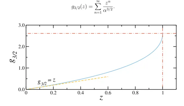
whereλ is the redefined de Broglie wavelength and the function g3/2(z) stands for the sum series
g3/2(z) = ∞
X
n=1 zα
α3/2. (1.10)
0 0.2 0.4 0.6 0.8 1
z
0.0 1.0 2.0 3.0
g
3/2
g
3/2≈
z
Figure 3 – Function g3/2 as a function of the gas fugacity represented by the blue line. The yellow line show that g3/2 can be approximated by a linear function for low values of z.
In Fig. 3, the g3/2(z) sum is plotted as a function of the gas fugacity and is represented by the blue solid line. For low values of z, which corresponds to the high temperature and low density limits, the g3/2 function presents an almost linear behavior and can be well approximated by g3/2 ≈z, as illustrated by the linear function designed by the yellow dashed line. As a consequence, in the classical regime, the chemical potential may be well described by
µ≈ −3
2kBT ln
mkBT 2π¯h2n2/3
!
. (1.11)
is represented by the interception of the red dashed-dotted lines in Fig 3. Although the right side of the Eq. (1.9) presents this bounding condition, the left side does not and thus, the limiting condition nλ3 ≤ζ(3/2) is not physical. This comes from the fact that the density of states g(ǫ) assigns zero weight to the ground state energy level and thus,n should be taken as the density of particles with non-zero momentum. Therefore, as the temperature (density) is decreased (increased) the left side of the former equation becomes higher, until it reaches its maximum value, g3/2(1) = 2.612. At this point, the chemical potential energy equates to the ground-state energy of an ideal gas, characterized by zero momentum ~k= 0. Beyond this limit, any excess of particles goes into the ground-state energy states macroscopically occupying it and therefore, giving rise to the BEC phase. The critical temperature follows from Eq. (1.9) for z = 1, where the right-hand side of Eq. (1.9) becomes equal to ζ(3/2) = 2.612,
Tc = 2πh¯2 kBm
n
2.612
2/3
. (1.12)
Below the critical temperature Tc, the condensed fraction of particles can be achieved by the particle conservation principle, where the total number of particlesN is a sum between all particles with zero momentum Nk=0 and those with non-zero momentum, which obeys expression Nk6=0 =V g3/2/λ3. The condensed fraction of particles of the system naturally follows from conservation of the total number of particles,
n0 n =
1−g3/2 λ3
=
"
1−T Tc
3/2#
, (1.13)
wheren0 andnaccounts for the condensed and uncondensed densities. A sketch of density-temperature phase diagram is shown in Fig. 4, where the blue background represents the condensed state and the red one stands for the gas phase. The origin of the Bose-Einstein
T
nT
3/2
=
c
ons
t
n
Condensed
Phase
Gas
Phase
Figure 4 – Phase diagram of Bose-Einstein condensation in the density-temperature plane.
and not by their inter-atomic interactions. Actually, one should expect interactions to spoil such phase transition, since under required temperature and density conditions, any set of particles would condense into solid state. Fortunately, current set of experiments has proved that such phase transition is robust enough so that, even in the presence of interactions and external confining potentials a gas can Bose condense (BURNETT MARK EDWARDS, 2008). However, a price has to be paid: in order to avoid the solid state of matter, the condensed phase must be achieved under the metastable phase of a very dilute gas, limiting, therefore, the visualization lifetime.
1.1.3 Path towards BECs
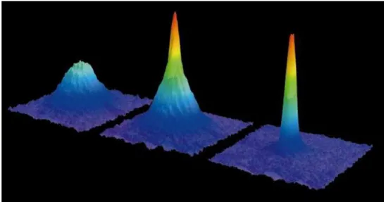
Because this was a theory without an experimental example at the time of its prediction, the BEC phenomenon did not received the proper and deserved attention. In fact, most physicists of that time, including Albert Einstein, took such idea as a mathematical pathology of non- interacting systems, which has nothing to do with the physical reality and, therefore, could never be realized experimentally. Moreover, except for 4He, at required densities and temperatures, all materials resides in its solid state and atoms are not delocalized as required by BEC theory. The closest evidence of Bose-Einstein condensation in nature was in the superfluid phase of helium isotope 4He (forT ≤2.17), found only later in 1937, which London tried to explain as a condensation phenomenon distorted by the presence of strong interactions between helium atoms (LONDON, 1938). London’s assumption was supported by a similar λ- point transition of the specific heat at an acceptable close critical temperature of 3.13 K, strengthening the link between BEC and superfluidity, (FEYNMAN, 1957; KAPITSZA, 1938; ALLEN, 1938). Further, more precisely in 1957, the BEC assumption was, again, taken as the main mechanism behind the microscopic explanation of superconductivity phenomena provided by Bardeen, Cooper and Schrieffer theory (BCS theory) (BARDEEN; COOPER; SCHRIEFFER, 1957). In BCS model, mediated by electron-phonon interactions, a weak effective attraction between electrons inside the superconducting material correlates electrons in pairs leading to the instability of Fermi sea. Because these pairs behave as bosonic particles, they could also Bose condense, exhibiting an electronic superfluidity (superconductivity) when subjected to sufficiently low temperatures. Subsequently, the BCS mechanism was used to explain the superfluid phase of the fermionic isotope of helium, 3He, which, despite presenting a half-integer spin, could also undergo through a Bose-Einstein phase transition by the same pairing mechanism (OSHEROFF; RICHARDSON; LEE, 1972; OSHEROFF et al., 1972; LEGGETT, 1972).
Figure 5 – Observation of Bose-Einstein condensation by means of absorption imaging technique, where the absorption is illustrated as a function two spatial directions for temperatures above, just below and well below the critical temperature, respectively illustrated in pictures from the left- to right-hand side. Figure retrieved from Ref. (DURFEE; KETTERLE, 1998).
al., 2009; LU et al., 2011), comprising different inter-particle interaction schemes, such as the contact, dipolar (LU et al., 2011) and even the spin-orbit coupling interactions(LIN; JIMENEZ-GARCIA; SPIELMAN, 2011). In fact, differently from the ideal Bose gas, alkali atoms in a magnetic trap do interact with each other, repelling (attracting) at short (large) interatomic distances. Usually, due to the gas diluteness, interactions are well described by a Lennard-Jones potential and theoretically modeled by a short-range contact interaction (HUANG; YANG, 1957; LEE; HUANG; YANG, 1957), governed by the s-wave scattering
length a (PETHICK; SMITH, 2002),
Vi(~r−~r′) = 4π¯h 2
a
m δ(~r−~r
′). (1.14)
The interaction strength can be experimentally tunned by means of an externally applied magnetic field, in a Feshbach resonance process, where quasibound molecular states share the same energy as an unbound state and thus couples resonantly to the free state of the colliding atoms (INOUYE et al., 1998; CHIN et al., 2010). The closer this molecular level lies with respect to the energy of two free atoms, the stronger the interaction between them. In fact, this resonance mechanism has strong influence on elastic collisions and because incoming atoms and quasibound states have different spin arrangements, the magnetic field becomes a powerful tool in order to control such interactions.
on the hyperfine spin states structure, have allowed the realization of multi-component BECs, where the macroscopic occupation occur in multiple spin substates (MYATT et al., 1997; HALL et al., 1998). Further, multi-component BEC was also observed to occur in mixtures of different isotopes of the same(PAPP; PINO; WIEMAN, 2008) and different atomic species (FERRARI et al., 2002; MODUGNO et al., 2002; THALHAMMER et al., 2008). As we shall see further in this thesis, multi-component BECs have a much richer physics and are far from being just a trivial extension of the single-component case.
1.1.4 Theoretical description of an interacting Bose gas
The collective behavior of particles lies in the heart of condensation phenomenon. In fact, for inherent quantum effects to be observed in a macroscopic scale, a large number (usually between 104 −106 atoms) of particles is required (ANNETT, 2004). Therefore,
a complete description of physical properties of realistic BECs would then require the solution of, at least, thousands coupled Schrödinger’s equations, which is numerically challeging nowadays. Then we must be satisfied with only an approximate understanding of how the Schrödinger equation could lead to solutions that would indicate a similar behavior to those observed experimentally. Fortunately, an approximate understanding might be achieved under the assumption of mean-field theory for weakly interacting systems, which yields to a Schrödinger-like equation, known as the Gross-Pitaevskii equation.
1.1.4.1 Second quantization and the many-body Hamiltonian
In the single-particle wave mechanics, the quantum mechanical formalism is usually developed over the eigenstates of position ˆx and momentum ˆpoperators. However, expanding up the formalism in order to account for many-body quantum objects leads to an ambiguity of eigenstates as a result of the exchanging degeneracy. Because it violates the state vector unicity, restrictions might be imposed on vector space, limiting it to a subspace that is invariant under the permutation of labels (SAKURAI; NAPOLITANO, 2011). At the end, the resulting basis might not contain individual information of each system particle, since, even in theory, this information is lost during the time evolution of the system (MERZBACHER, 1998).
One of the most elegant ways to avoid ambiguity on many-body quantum space proceeds by means of the introduction of a linear operator ˆψ(~r), which resembles the annihilation operator ˆa commonly used in quantum harmonic oscillator formalism (ROBERTSON, 1973). The quantum fieldψ depends on vector position~r and obeys, as the only requirement, the symmetry properties of particles, which is done by imposing the following (anti-) commutation relation that ˆψ(~r) and its hermitian conjugate ˆψ†(~r) must
obey,
ˆ
ˆ
ψ†(~r) ˆψ†(~r′)∓ψˆ†(~r′) ˆψ†(~r) = 0, (1.15b)
ˆ
ψ(~r) ˆψ†(~r′)∓ψˆ†(~r′) ˆψ(~r) =δ(~r−~r′), (1.15c)
where δ(~r−~r′) is the Dirac delta function and the upper (lower) signal stands for bosonic
(fermionic) particles. Operators ˆψ(~r) and ˆψ†(~r) provide a convenient and useful basis for
representing many-particle states and many-body operators. In fact, it leads to a less superfluous notation than symmetrized and anti-symmetrized wave functions. The analogy between ˆψ and ˆa becomes clear by defining an hermitian operator
ˆ N ≡
Z
d3rψˆ†(~r) ˆψ(~r), (1.16)
where, the employment of ˆψ must guarantee the existence of at least one non-trivial eigenstate |φi, with a corresponding eigenvalue nφ defined by ˆN|φi=nφ|φi. Through the application of commutation relations [N,ψˆ(r)] =−ψˆ(~r) and [N,ψˆ†(r)] = ˆψ†(~r) on state
|φi, one may derive
ˆ
Nψˆ(~r)|φi= (nφ−1) ˆψ(~r)|φi, (1.17a)
ˆ
Nψˆ†(~r)|φi= (nφ+ 1) ˆψ†(~r)|φi. (1.17b) States ˆψ(~r)|φi and ˆψ†(~r)|φi are, therefore, identically zero or new nontrivial eigenstates
of operator ˆN with eigenvalues nφ−1 and nφ+ 1 respectively. The expected value of operator ˆN in the state |φi establish a lower bound for eigenvalues, nφ ≥ 0, and then, from the existence of an arbitrary nontrivial eigenstate |φi of N, a nontrivial eigenstate
|0i of ˆN must exist, satisfying the equation ˆ
ψ(~r)|0i= 0. (1.18)
The decreasing sequence of eigenvalues has integral spacing and must have zero as the lower bound value, making non-negative integers the only accessible numbers: nφ= 0,1,2,3.... In turn, the creation operator ψ†(~r) may be used to remove almost completely the need of
state vector, allowing to retain only the special state |0i. In fact, any other eigenstate of ˆN can be achieved by successive applications of ψ† on |0i:|0i, ˆψ†(~r
1)|0i, ˆψ†(~r2) ˆψ†(~r1)|0i, etc. This enable to use operators rather than vector states to describe the physics, which is advantageous since operators ψ† andψ carry the symmetry properties of particles. In fact,
eigenfunctions are highly degenerate, indeed, statesψ†(~r)|0iandψ†(~r′)|0iare, for example,
associated with the same eigenvalue n= 1, even if~r6=~r′. The orthogonality of these states
is satisfied under two circumstances:(i) If their corresponding eigenvalue ofN are different or (ii) if their corresponding eigenvalues are the same, but their arguments~r1, ~r2, ..., ~rn are not all the same. The last condition can be expressed mathematically, in the two-particle context, as
h0|ψˆ(~r1) ˆψ(~r2)...ψˆ†(~r′2) ˆψ†(~r′1)|0i=δ(~r1−~r1′)δ(~r2 −~r2′)±δ(~r1−~r2′)δ(~r2 −~r1′). (1.19)
Except for state |0i, eigenstates of ˆN can not be normalized, since Dirac delta function diverge at the origin. Still, following a similar procedure of free-particles in the standard wave mechanics formalism, normalized states might be achieved. For instance, through an educated guess, the single-particle non-normalized state may be written as
|Ψ1i= ˆψ†(~r1)|0i. (1.20)
Actually, this is exactly the same process of adding one quantum of energy in the case of a harmonic oscillator. However, as we shall see further, it now means an addition of one particle in space at position ~r1. The norm,hΨ1|Ψ1iis not well defined, since
hΨ′1|Ψ1i=h0|ψˆ(~r′1) ˆψ†(~r1)|0i= =δ(~r1−~r′1),
(1.21)
diverges when Ψ = Ψ′. However, with the experience provided by the standard formalism, a
general single-particle state may be contructed as a linear spatial superposition of position eigenfunctions
|Ψ1i=
Z
d3r1Ψ(~r1) ˆψ†(~r1)|0i, (1.22) where Ψ(~r1) is a weight factor. Substituing last equation in the time-dependent Schrödinger equation, it turns out that Ψ(~r1) is actually the wave function of a free particle in the wave conjecture of quantum mechanics. Similarly, the N-particle state may be defined as
|Ψni= 1
√
n!
Z
d3r1...
Z
d3rnΨ(~r1, ..., ~rn) ˆψ†(~rn)...ψˆ†(~r1)|0i. (1.23)
The meaning of such assumption becomes clear when the state|ΨNiis subjected to the application of operator ˆN. In fact, recalling the commutation that [ ˆN ,ψˆ†(~r)] = ˆψ†(~r),
or similarly ˆNψˆ†(~r) = ˆψ†(~r)( ˆN + 1), it is possible to derive from direct application of ˆN
on |Ψni the eigenvalue equation ˆ
N|Ψni=n|Ψni, (1.24)
ˆ
N as a number operator, where the special state |0i plays the role of a vacuum state, characterized by the absence of particles. It also turns out, through direct application on |Ψni, that operators ˆψ†(~r) and ˆψ(~r) may create a particle or destroy a partice at ~r, leading to a new eigenstate of ˆN and justifying the educated guess for then-particle state. Because the application of ˆψ(~r) and ˆψ†(~r) to any linear combitation of eigenstates of ˆN
always generate a vector inside this same subspace, the closure condition is satisfied and subspace vectors |0i, ˆψ†(~r
1)|0i, ˆψ†(~r2) ˆψ†(~r1)|0i, ..., ˆψ†(~rN)...ψˆ†(~r2) ˆψ†(~r1)|0iindeed form a basis in Fock space.
By repeated applications of the annihilation operator in the state |Ψni and using the normalization rule for the vacuum state, it is possible to derive the state in the wavefunction formalism Ψn(~r1, ..., ~r2) in terms of Fock state|Ψni
Ψn(~r1, ..., ~rn) = 1
√
n!h0| ˆ
ψ(~r1)...ψˆ(~rn)|Ψni, (1.25) which carries permutation (anti-)symmetry in (anti-)commutation relations obeyed by creation and annihilation operators. Despite we are avoiding to work with Ψn(~r1, ..., ~rn), due to the ambiguity of the wavefunction description, the former equation allows one to prove the equivalence between the field operator and wavefunction formalisms (ROBERTSON, 1973). This means that the transformation that takes a Hamiltonian from wavefunction space to the Fock space preserves the physical result. In a many particle system, where particles are subjected to an external potential Ve(~r) and interact with each other through the potential Vi(~r, ~r′), the Fock-space Hamiltonian may be defined by (ROBERTSON,
1973)
ˆ
H =Z d3rψˆ†(~r)
"
−¯h
2 2m∇
2+Ve(~r)
#
ˆ
ψ(~r) + 1 2
Z
d3rd3r′ψˆ†(~r) ˆψ†(~r′)Vi(~r, ~r′) ˆψ(~r) ˆψ(~r′).
(1.26)
The first and second terms account for all single-particle processes that might occur and operate on a many particle state. In fact, both operators represent a sum over all spatially avaiable process in which a particles is removed from position~r, submitted to the single-particle matrix element and then replaced at position~r. In turn, the last term represents the energy associated with the atom-atom interaction, where the coefficient 1/2 avoid double counting pairwise interactions. The equivalence between theses operators and operators in wave mechanics formalism may be derived from their direct application on the n-particle state |Ψni. As previously pointed out, for evaporatively cooled gases, like in mixtures of rubidium and caesium, the de Broglie wavelength of atoms is very large compared with length scales of interatomic forces and are mainly described by two-body scattering, which, under low-energy condition, may be modeled by contact interactions, Vi =gδ(~r−~r′), whereg is proportional to the s-wave scattering length as and is defined by
g = 4π¯h 2
In fact, this is a good approach for the most cases of BECs and it is of the main interest for the work presented in this thesis.
1.1.4.2 Bogoliubov approach
Because, the condensation occur in a single state of momentum space, it is advantageous to perform a change of basis and write operators ˆψ(~r) and ˆψ†(~r) in terms of
operators which annihilate and create particles in momentum space, designed by ˆa~k and ˆ
a~k† (LANCASTER; BLUNDELL; BLUNDELL, 2014). The basis change can be performed under a Fourier transform of momentum space operators, which leads to
ˆ
ψ(~r) = √1
V
X
~k
ei~k·~ra~k, (1.28)
ˆ
ψ†(~r) = √1
V
X
~k
e−i~k·~ra~k†. (1.29)
After straightfoward calculations, the ~k-space hamiltonian describing Bose particles in absence of external potential and interacting with each other through contact mechanism becomes,
ˆ H =X
p ˆ p2 2maˆ
†
pˆap+ g 2V
X
kpq ˆ
a†p−qˆa†k+qˆakˆap, (1.30)
where the sum goes over all momentum states. Despite it provides a general way to discuss many-body systems in a much more simplified picture than in usual wave mechanics formalism, solving Eq. (1.30) for macroscopic samples is still an impossible task and then requires subsequent approximations. In fact, diagonalizing the interaction contribution term is still very tricky when a large amount of particles is considered. To overcome difficulties provided by the Hamiltonian interaction term, Bogoliubov proposed to explore the consequences of the macroscopic occupation of the ground state. Instead of using exact properties obeyed by ˆa† and ˆa when applied to the ground-state |Ωi,
ˆ
a~k=0|ΩN0i=
q
N0|ΩN0−1i, (1.31)
ˆ a~k†
=0|ΩN0i=
q
N0+ 1|ΩN0+1i. (1.32)
condensate fraction represents only 8% of the total number of particles (PENROSE; ONSAGER, 1956), which explains nonconformities between experimental observations and the present microscopic theory. Therefore, under sufficiently low temperatures, it would be reasonable to state that
ˆ
a~k=0|ΩN0i=
q
N0|ΩN0i, (1.33)
ˆ a~k†
=0|ΩN0i=
q
N0|ΩN0i. (1.34)
The error associated with Bogoliubov’s prescription is of the order of the commutator [ˆa0,ˆa†0] = 1 and is much smaller than the avarage values of creation and annihilation in macroscopically occupied ground-state and therefore, may be neglected. Within this approach, a spontaneous global symmetry break occur. In fact, the U(1) symmetry is lost and consequently the particle number is not conserved. However, the hamiltonian could be reduced to its simplest form
ˆ
H ≈ gN 2 0 2V +
X
p6=0 p2 2m +
2gN0 V
!
ˆ
a†pˆap+ gN0 2V
X
p6=0
ˆ
a†paˆ†−p + ˆapˆa−p
= 1 2gn
2 +X
p6=0 p2 2m +ng
!
ˆ
a†pˆap+1 2
X
p6=0
ngˆa†paˆ†−p+ ˆapˆa−p
.
(1.35)
Here, n=N/V stands for the total density of particles and the total number of particles N was taken as the sum of ground state particles N0 and all the rest occupying excited states,
N =N0+
X
p6=0 ˆ
a†pˆap. (1.36)
The Hamiltonian of Eq. (1.35) may be exactly diagonalized by means of a canonical trans-formation, where creation and annihilation particle operators are replaced by Bogoliubov quasiparticle operators ˆα†k and ˆαk, defined by
ˆ
αk =fkˆak+gka†−k and ˆα−†k=gkˆak+fka†−k. (1.37)
where fk and gk are real functions and must be such that preserve commutation relations originally obeyed by creation and annihilation operators, [ˆαk,αˆ†−k] =f2
k −gk2 = 1. ˆαk and ˆ
α†−k actually account for exchanging particles with the system ground-state and provide, under an unitary transformation, a proper basis where the Hamiltonian may be exactly diagonalized. The ground-state of such approximated Hamiltonian enabled Bogoliubov to describe the energy dispersion of quasi-particle excitations for weakly interacting set of bosonic particles, named Bogolons. The energy dispersion may be expressed as following
ǫ(~p) =
v u u t p2 2m p2
2m + 2ng
!
, (1.38)