www.ann-geophys.net/27/2491/2009/
© Author(s) 2009. This work is distributed under the Creative Commons Attribution 3.0 License.
Annales
Geophysicae
Numerical simulations of thermospheric dynamics: divergence as a
proxy for vertical winds
S. L. Cooper1, M. Conde2, and P. Dyson1
1Department of Physics, La Trobe University, Melbourne, Victoria, Australia 2Department of Physics, University of Alaska, Fairbanks, AK, USA
Received: 20 June 2008 – Revised: 14 May 2009 – Accepted: 1 June 2009 – Published: 22 June 2009
Abstract. A local scale, time dependent three-dimensional model of the neutral thermosphere was used to test the appli-cability of two previously published empirical relations be-tween thermospheric vertical wind and velocity divergence, i.e., those due to Burnside et al. (1981) and Brekke (1997). The model self-consistently solves for vertical winds driven by heat and momentum deposited into the neutral atmosphere by high latitude ion convection. The Brekke condition accu-rately mimicked the overall “shape” of the three-dimensional model vertical wind field although, as written, it consistently overestimated the vertical wind magnitude by a factor of ap-proximately 5/3, for the heating scenarios that we consid-ered. This same general behavior was observed regardless of whether the forcing was static or rapidly changing with time. We discuss the likely reason for the Brekke condi-tion overestimating the magnitude of our vertical winds, and suggest an alternative condition that should better describe vertical winds that are driven by local heating. The appli-cability of the Burnside condition was, by contrast, quite variable. During static heating, both the magnitude and the sign of the model vertical winds were predicted reliably at heights above those of maximum energy and momentum de-position per unit mass. However, below the thermal forc-ing, the Burnside condition predicted vertical winds of the wrong sign. It also introduced significant artefacts into the predicted vertical wind field when the forcing changed sud-denly with time. If these results are of general applicabil-ity (which seems likely, given the way these relations are derived) then the Burnside condition could usually be used safely at altitudes abovehmF2. But it should be avoided
be-low this height at all times, and even at high altitudes during periods of dynamic forcing. While the Brekke condition (or our modified version of it) could likely be used in all
circum-Correspondence to:S. L. Cooper ([email protected])
stances, there are few experimental scenarios for which this would be useful. This is because evaluation of the Brekke condition would not usually be possible unless the vertical wind was already known in advance.
Keywords. Atmospheric composition and structure (Pres-sure, density, and temperature) – Ionosphere (Ionosphere-atmosphere interactions) – Meteorology and atmospheric dy-namics (Thermospheric dydy-namics)
1 Introduction
The most difficult wind component to measure in Earth’s thermosphere is the vertical, for two reasons. First, verti-cal winds have smaller speeds than horizontal winds. Sec-ond, ground-based remote sensing of thermospheric verti-cal wind is usually restricted to viewing solely in the zenith, which yields limited geographic coverage. These difficulties have motivated various attempts to infer thermospheric ver-tical winds indirectly from other data. For example, Burn-side et al. (1981) describe a simple relation between verti-cal wind and the divergence of the two-component horizon-tal wind field. However, mathematical derivation of this re-lation requires a number of assumptions that may not hold in the real atmosphere. Brekke (1997) presents an alterna-tive relation, in this case between the total divergence of the three-component wind field and its vertical component.
wind parallel to their look direction, a single ground-based Doppler spectrometer can unambiguously measure vertical wind only when observing directly overhead. Furthermore, to derive all three wind components, an FPI must observe in at least two additional linearly independent off-zenith direc-tions. In a common scenario, narrow-field observations are taken in a total of five directions: zenith, plus north, east, south and west at a 20◦to 30◦ elevation angle. Subject to some assumptions, all three wind components can then be derived, together with an estimate of horizontal divergence. Alternatively, a number of all-sky imaging FPIs have been developed (Rees and Greenaway, 1983; Biondi et al., 1995; Conde and Smith, 1997; Ishii et al., 2002), however most of these cannot measure vertical winds directly in the zenith because the dispersion of wavelength with zenith angle is in-finite at the center of the Fabry-Perot ring pattern. The ex-ception to this is the all-sky instrument described by Conde and Smith (1997), which measures spectra from all portions of the sky by scanning the etalon gap over time.
When observing the 630 nm emission from atomic oxygen at around 240 km altitude, a five-direction observing scheme would sample thermospheric regions that are horizontally separated by around 500 km. Despite the thermosphere’s very high kinematic viscosity, all-sky imaging FPI observa-tions (Conde and Smith, 1998, for example) have observed relatively small scale structure in the wind field. Using a Doppler Imaging Fabry-Perot spectrometer Batten and Rees (1990) reported observations of structures in the F-region wind field at spatial scales as short as∼50 km, with
tempo-ral scales as short as∼10 min. They concluded that a spatial resolution much better than 500 horizontal km is required to resolve the smallest scale wind features that occur. The goal of the present study is to model thermospheric dynam-ics with adequate resolution to study features at these spatial and temporal scales which, until now, has not usually been feasible.
The vertical component of the thermospheric wind field is the one expected to exhibit most structure over small spa-tial scales. Smith (1998) reviewed the recent understanding of such vertical winds. Whilst he noted that thermospheric vertical wind speeds in excess of 100 m s−1 have been ob-served by a number of groups, the mechanisms that produce such large speeds are not well understood. Deng et al. (2008) have completed some modelling regarding the generation of such vertical winds and present a possible mechanism. How-ever, the current study is concerned only with more common vertical wind speeds up to about 10 ms−1, which are an
or-der of magnitude smaller than typical horizontal winds, and are well within the speed range for which possible gener-ation mechanisms are known. The typical 1−σ uncertainty of FPI wind measurements is around 5 ms−1which is 50% of the vertical wind speeds of interest here. Such large relative errors are obviously undesirable for observations; an alter-native experimental procedure for measuring vertical winds would be very appealing. Two possible alternative methods
have been tested in this study, the “Burnside” and “Brekke” conditions, which are defined below.
There are two components of vertical winds that persist in the thermosphere and contribute to the total vertical wind. The first component is the “barometric” component which is driven by the expansion and contraction of the thermosphere due to solar heating, effectively the atmosphere’s “breath-ing” motion. The second is everything else that drives ver-tical winds, this includes the “divergence” component that arises from diverging and converging horizontal winds. Due to the solar heating pressure gradients will drive horizontal winds and to preserve mass continuity vertical winds will arise (Rishbeth et al., 1969). Upwelling can also be driven by intense local heating, such as Joule heating or particle pre-cipitation. The present study is concerned with Joule heating and the subsequently driven winds, in fact tidal motions are not included in the model.
The atmosphere’s horizontal divergence and vertical wind are coupled through the requirement to conserve mass, a con-dition described by the continuity equation:
∂ρ
∂t + ∇ ·(ρu)=0 (1) where t is time, ρ is the mass density and u is the 3-component neutral wind velocity vector. Using this and as-suming hydrostatic equilibrium, it is straightforward to de-rive the “tendency equation” (Hess, 1959):
uz(z)= 1 ρ (z) 1 g ∂p(z) ∂t +
Z ξ=∞
ξ=z
∇h·[ρ (ξ )uh(ξ )]dξ
(2) wherep(z)is the pressure at heightz,ξ is a dummy variable for integration over altitude,uh is the horizontal wind, and
∇h= ∂
∂xbx+ ∂
∂ybyis the horizontal del operator.
Equation (2) does not in general produce a simple and uni-versal relationship between vertical wind and horizontal di-vergence. This is partly because the time derivative of pres-sure and the horizontal gradient of density are also involved in the coupling. But even if we simplify Eq. (2) by assuming that ∂p∂t =0 and ∇h·ρ=0, knowledge of horizontal diver-gence at one location is not in general adequate to predict the vertical wind there. However, by introducing two further assumptions, Burnside et al. (1981) obtained the following simple approximation, referred to here as the “Burnside con-dition”:
uz=H ∂ux ∂x + ∂uy ∂y
=H∇h·u (3) whereHis the scale height.
The two additional assumptions used by Burnside et al. (1981) in deriving Eq. (3) from Eq. (2) are:
– The horizontal divergence of the horizontal wind is in-dependent of height: ∂z∂ (∇h·uh)=0
– The atmosphere is isothermal at heights abovez: ∂T
The Burnside condition has been tested in several obser-vational studies – with differing conclusions. These in-clude comparisons with observational data at mid-latitudes (Biondi, 1984; Sipler et al., 1995) and at high latitudes (Crickmore, 1993; Smith and Hernandez, 1995). Biondi (1984) used an FPI to observe the two-dimensional horizon-tal wind field and the corresponding overhead vertical wind. It was found that vertical winds were indeed associated with horizontally divergent flows but the Burnside condition over-estimated the vertical winds. By contrast, Sipler et al. (1995) determined that average vertical winds during geomagnet-ically quiet times were larger than the Burnside condition would suggest. At high latitudes Crickmore (1993) observed that the Burnside condition underestimated the magnitudes of the measured winds by a factor of approximately two. Smith and Hernandez (1995) compared the vertical winds observed within the polar cap to those predicted by the Burn-side condition and also found that the magnitude of the ac-tual vertical winds were double those predicted. However, they found that the sign of the observed vertical wind was opposite to that predicted by applying the Burnside condi-tion to the observed horizontal divergence – which is a much more serious discrepancy. Nevertheless, there was at least a correlation between the two quantities. However, it was con-cluded by Smith (1998) that the Burnside condition appears inappropriate at high latitudes.
An alternative relation between vertical wind and velocity divergence is given by Brekke (1997, p. 260) and referred to here as the “Brekke condition”:
uz=γ H∇ ·u (4)
whereγis the adiabatic constant,cp/cv. Unlike the Burnside condition, the Brekke condition uses the total divergence in the neutral wind field to infer vertical wind speed.
The Brekke condition can be derived from the mass con-servation equation (Eq. 1), subject to some approximations. First, it is assumed that the atmosphere is quasi-static allow-ing the time derivative of density to be removed. Further ap-proximations used include assuming the horizontal gradients in density are zero, the ideal gas law holds, hydrostatic equi-librium holds, and that the vertical wind displaces air parcels adiabatically. All but the last of these approximations are reasonable over most spatial and temporal scales of interest. The adiabatic assumption may or may not be reasonable – depending of course on whether the vertical motion is driven by local heating.
The existence of some relationship between divergence and vertical wind has been observationally verified by the studies cited above, but the best form for this relation re-mains unclear. There is thus considerable practical motiva-tion to determine which condimotiva-tion best describes the actual behavior of the real atmosphere. This was the objective of the present study, in which we used a high spatial resolution and fully self-consistent numerical model of the neutral
thermo-sphere to compare model vertical winds with those predicted by both the Burnside and Brekke conditions.
Numerous global-scale general circulation models of the atmosphere have been developed, Fuller-Rowell and Rees (1980), Dickinson et al. (1981), Richmond et al. (1992), Har-ris (2001) and Ridley et al. (2006) for example. In one such study, Rees et al. (1984a) applied a global scale model to sim-ulate the thermospheric vertical wind field on specific days, and compared the results to corresponding observational data (Rees et al., 1984b). A major problem with this approach is that the global nature of these models precludes them from resolving dynamics on the scales that are likely to be impor-tant for driving vertical winds that are the focus of the work reported here. One global model that can potentially address dynamics at high resolution is the nested grid model of Wang et al. (1999). This model allows a region of higher spatial resolution to be nested into the global-scale model. The ini-tial Thermosphere-Ionosphere Nested Grid (TING) model of Wang et al. (1999) contained only a one way coupling be-tween the global and nested model domains, with the coarse grid model affecting the nested model. The TING model now incorporates two-way coupling between the nested grid and the global grids (Wang et al., 2005). However, the externally specified fields usually do not have adequate resolution to match the scales being studied here.
More recently, Ridley et al. (2006) reported the de-velopment of the Global Ionosphere-Thermosphere Model (GITM) which can have very flexible spatial resolution, al-lowing for higher spatial resolution than previous global scale models. This model solves on an altitude based grid rather than a pressure based grid, which means that hydro-static equilibrium need not be enforced. This is an important feature of both the GITM and our model, however the GITM remains a global scale model. Deng and Ridley (2006) used the GITM with a spatial resolution of 2.5◦in latitude, 5◦in longitude and 0.25 of a scale height vertically to investigate various influences on the high latitude neutral winds. Al-though a similar region of the atmosphere was considered the neutral vertical winds were not the focus of this study.
be quite inappropriate. Deng and Ridley (2007) ran mod-els with varying spatial resolution in a study investigating possible reasons for the underestimation of Joule heating in global scale models. Sub-grid dynamics affected the strength and the positioning of the Joule heating in the low resolution models.
Some modelling of smaller scale structures has also been undertaken using 2-D models (Fuller-Rowell, 1985; Walter-scheid et al., 1985; WalterWalter-scheid and Lyons, 1992). Fuller-Rowell (1985) modelled the neutral wind response to forcing from electrodynamic features, both narrow and broad. The resolution of the nested regions of this model were similar to the resolution used in our current work. However, be-ing only a 2-D transient model most likely limited this study from capturing all the processes included in the present work. It is worth noting that the neutral wind and temperature re-sponses of both models do appear reasonably consistent. The temperature changes seen in both models are a few Kelvin in amplitude, and in both cases the vertical wind response is strongest about 10 min after a change in the forcing. Simi-lar responses were also observed in 2-D modelling work by Walterscheid et al. (1985), Walterscheid and Lyons (1992) and Chang and St.-Maurice (1991). Chang and St.-Maurice (1991) determined that advection of momentum and energy can dominate over local scales near the small scale forcing features.
The neutral wind response to a stable auroral arc was sim-ulated by Walterscheid et al. (1985). One interesting result was a region of cooling that arose near the arc soon after its appearance. Chang and St.-Maurice (1991) used a 2-D model of the upper atmosphere and compared results between an extreme case of forcing and a moderate case. In each case wave motions in vertical winds were observed, with the re-sponse to extreme forcing being much more pronounced, as expected. Non-linear terms in the governing equations were found to dominate in the extreme case, but play a lesser role in the moderate case.
More recently Sun et al. (1995) used a 3-D time dependant model to simulate the thermospheric response to diffuse au-rora. The resolution of the model was 170 km longitudinally, 75 km latitudinally and 5 km vertically. A 2-D version of the model was also run and the results showed that the 3-D model was more accurate in simulating the neutral wind response. The 2-D models were shown to generate zonal winds that were about twice the strength of the 3-D zonal winds, with the 3-D zonal winds being more representative of the realistic atmospheric response.
2 The model
The model used in this study employs the finite volume method (FVM) to solve a set of time dependent, non-linear coupled three-dimensional partial differential equa-tions. The model domain extends 1000 km in the zonal
direc-tion, 600 km meridionally and 300 km vertically. (The actual height range represented is 100 km to 400 km.) The resolu-tion of the model is 20 km zonally, 15 km meridionally and 750 m vertically. The reason for the high vertical resolution is that the model does not enforce hydrostatic equilibrium, which allows small scale waves to develop with short verti-cal wavelengths. Such waves are often observed, especially during the early time steps of a model run, before minor nu-merical inconsistencies associated with the boundaries have damped out.
Although the spatial resolution of the model is higher than previous 3-D studies, the authors cannot exclude the pos-sible existence of structures at even smaller spatial scales in the real atmosphere. The structure that we actually ob-serve in our simulations does not approach the model’s grid size, which suggests to us that the spatial resolution currently used is adequate for the phenomena that we are considering. Higher spatial resolution may well be required to model the response to even more localised forcing fields, but we have not yet studied behaviour at such scales.
There are five main equations that define the model: the three components of the momentum equation, the energy equation and the mass continuity equation. These are the familiar Navier-Stokes equations; the versions that are used in the model are listed below. Earth’s curvature is assumed to be unimportant over the limited spatial extent of the model domain, which allows a simple Cartesian co-ordinate system to be used. Effects of Earth’s rotation are included, by reten-tion of the Coriolis term in our momentum equareten-tion. 2.1 Momentum equation
The momentum equation used is: ∂(ρu)
∂t = − ∇ ·(ρuu)+ ∇
2(µu)
−ρνni(u−v)+ρg
−2ρ (×u)− ∇p (5) witht representing time,ρbeing the neutral mass density,u
is the neutral velocity vector,µis the co-efficient of viscosity, νnithe neutral-ion collisional frequency,vthe ion convection velocity vector, g the gravity vector, is Earth’s angular velocity vector andpis pressure.
The momentum equation (Eq. 5) describes the time rate of change of velocity, via terms that describe advection, viscos-ity, ion drag, gravviscos-ity, Coriolis and the pressure gradient. 2.2 Energy equation
The Energy equation is: ∂(ρe)
∂t = − ∇ ·(ρue)+ ∇
2(κe)+ρνni 2 (u−v)
2
The energy equation (Eq. 6) describes the time rate of change of energy, using terms describing advection, thermal diffusivity, Joule heating, work and viscous heating. Tem-perature is retrieved by dividing the energyeby the specific heat capacity at constant volumecv.
2.3 Mass continuity equation
The requirement for mass conservation is used to close the set of equations (Eq. 1). Terms in this equation correspond to the time rate of change of density and divergence of mass flux.
2.4 Predefined fields
Initial temperature and pressure fields are implemented from empirical fits to MSIS model fields (Hedin, 1991). This ver-sion of the model was used as we already had access to a working version of this code. While newer versions of the model are available this model is adequate for our purposes since our interest is in the changes produced by additional heating rather than trying to exactly match the atmospheric conditions at a particular time or location. The density field is obtained from these using the ideal gas law. These fields then evolve self-consistently as the model proceeds. The ion density and velocity fields are externally specified at all time steps. For the runs shown here, ion density peaked at 2×10¹¹m−3at an altitude of 300 km, and was specified with
a Chapman-like profile for convenience. The ion velocity (convection) field drives the neutral dynamics in the model, and is varied according to the problem of interest but there is only a one-way coupling of the ion convection with the neutral atmosphere. Ion velocity is purely horizontal, and is constrained to be (predominantly, due to discrete sampling) non-divergent. Thayer and Killeen (1993) showed that the ion convection is non-divergent to first order, although it is acknowledged that observations of divergent ion convection do exist (Andr´e et al., 2003). The ion convection used is a narrow channel flowing predominantly in the zonal (west-ward) direction and peaking at a speed of 800 ms−1, with a
kink partway along the channel. It has a similar geometry to the convection pattern used in an earlier model (e.g. Fig. 1 of Cooper and Conde, 2006), however it now extends up to 400 km in altitude and tails off below an altitude 130 km. The meridional width of the channel is approximately 150 km.
The model is based on differential equations whose so-lution only becomes unique when constrained by boundary conditions. However, inconsistent boundary conditions can introduce artefacts or worse, they can cause the model to fail. The boundary conditions used in the current study are as fol-lows: the normal derivatives of all parameters are set to zero on the side boundaries. On the bottom boundary the pres-sure and temperature are kept constant at their MSIS values, whilst the normal derivatives of the velocity components are each set to zero. On the top boundary the normal
deriva-tives of all quantities are set to zero except for pressure, the gradient of which is set to ensure hydrostatic equilibrium. Inconsistencies (such as discontinuous second spatial deriva-tives) initially occur at the boundaries, launching waves and other small artefacts. Because of this, the model is initialised by running it for a few hours of model time with no forc-ing, which allows the artefacts to dampen out. The resulting fields, with neutral velocities of only fractions of ms−1, are then used as starting conditions for subsequent model runs, with the forcing of interest being turned on a few time steps later.
We have investigated the performance of the Burnside and Brekke conditions, with high spatial and temporal resolu-tion, by driving the neutral dynamics with ion convection and comparing the resulting vertical winds with those pre-dicted by the two conditions. Specifically, the ion convec-tion pattern was initially started with a kink 300 km from the eastern end of the model where it was maintained for 5400 model seconds after which time it was moved (instanta-neously) some 400 km westward, where it remained for all of the following 5400 model seconds. The instantaneous move-ment of the ion convection kink was implemove-mented to allow an assessment of the impulse reaction of the model. This al-lows a comparison between a “static” convection pattern and a time-varying, disturbed pattern.
The time step used in the model was 1 model second, however the fields were written out every 60 model seconds (the current temporal resolution of the model output). It was found that time steps larger than 1 model second could yield unacceptably large acoustic Courant numbers, which would cause the model to become unstable and fail. A similar pro-cess was identified by Chang and St.-Maurice (1991); the time step taken by their model was half a model second.
3 Results and discussion
Ion convection is the only external momentum source in the model. It also deposits energy by Joule heating. For the cur-rent model runs, the ion convection was simply turned on at time zero. Since the initial fields were obtained from a steady state model run with no convection, this meant the model essentially experienced an instantaneous step change in convection, rather than a gradual build up in speed. 3.1 Zonal wind and temperature responses
Neutral wind speeds near the convection channel began in-creasing as soon as the ion-drag forcing was turned on. As expected, the largest wind response appeared in the zonal component, because this is the direction parallel to the major ion-drag forcing. It is interesting to note that the maximum zonal velocity, after 3 model hours, was 291 ms−1westward which is∼36% of the ion convection speed. An example of
Fig. 1. The time evolution of the zonal component of the neutral wind field at an altitude of 300 km. The position of the data used in this figure is shown as a circle in Fig. 2.
similar to the results obtained by Walterscheid et al. (1985) who observed the maximum velocity was some∼40% of the
zonal electric field drift velocity. The winds are negative here because the ion convection is moving in the westward di-rection. It must be noted that the zonal winds may increase further but the model run was concluded after 3 model hours, however modelling by Deng and Ridley (2006) indicated that it took 3 h for the neutral winds at an altitude of 300 km to approach their final values or 4 h at 200 km. Our simula-tions show that it is the viscosity term that mostly limits the steady-state neutral winds at∼40% of the ion speed.
After 5400 model seconds the temperature change at an altitude of 300 km had a magnitude of∼19 K, as shown in Fig. 2. The “convection channel” can be seen and there is some heating in the convection channel prior to the kink and interestingly there is some cooling in the channel after the kink. Large temperature changes occurred near side bound-aries of the model domain, but these are presumed to be a consequence of imperfect boundary conditions, rather than real physical processes in the atmosphere. Of specific inter-est to this study is the change in the temperature in or near the ion convection. Heating occurred in the channel upstream of the convection kink. This is expected, as Joule heating should be strongest at the location of greatest ion-neutral ve-locity difference. However, just downstream of the kink the temperature was actually lower than it was at the start of the model. This region of cooling coincided with a region of large (total) divergence in neutral wind, which is the likely cause of the cooling. If the work term in the energy equation (Eq. 6) was large enough this would cause the region to cool, as appears to be the case in this region. Regions of cooling have also been observed by Walterscheid et al. (1985). In their case these regions were thought to be due to either
ver-Fig. 2.A plot of the difference (from time equals zero) in temper-ature at an altitude of 300 km after 5400 model seconds. The zonal direction spans 1000 km and the meridional direction spans 600 km as shown. The black circle represents the position of the data used in Fig. 1 whilst the convection channel is outlined by the black lines.
tical displacements of air parcels or from dynamics resulting from acoustic disturbances.
3.2 Vertical wind response
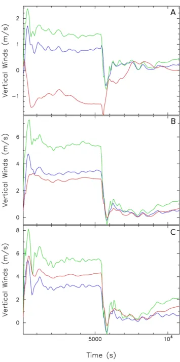
We focus here on three altitudes at which we examine the applicability of the Burnside and Brekke conditions. These are 225 km, 275 km and 325 km. These three altitudes span the height range over which momentum forcing maximized. Upward wind commenced in our model as soon as forcing was initiated. Vertical speeds maximized 6–7 min after the start of the forcing, before settling down. This rapid re-sponse has been noted previously by others. Walterscheid et al. (1985) observed that the vertical winds maximised af-ter 8 min of forcing, while plots from Fuller-Rowell (1985) show that the vertical wind was largest after 10 min (when compared to plots after 60 and 180 min). Both of these stud-ies used two-dimensional models. This characteristic tem-poral response is understood to be an indication of the time scale over which the atmosphere reasserts hydrostatic equi-librium following the initial shock from the forcing. There was another spike in vertical wind following the move of the convection kink at 5400 model seconds. Vertical winds once again maximised 6–7 min after this perturbation, then gradu-ally settled down.
3.3 The Burnside and Brekke conditions
runs (not presented here) with larger ion densities and con-vection speeds have generated substantially stronger vertical winds, but the conditions simulated in the present model run were intentionally modest. The key point in panel (a) is that the Burnside condition predicts downward winds at 225 km altitude, when the model vertical wind was flowing upward. This discrepancy is not too surprising; the Burnside condi-tion only allows upward vertical wind to be associated with divergent horizontal flow, whereas a convective upwelling cell would include horizontal divergence of both signs – con-vergent at the base and dicon-vergent at the top. As described earlier, instances of anti-correlation between observed ver-tical winds and the corresponding Burnside prediction have been verified by observation (Smith and Hernandez, 1995).
Panels (b) and (c) (of Fig. 3) show that the Burnside ver-tical winds above 225 km are, for the most part, quite ac-curate. They mimic the variations in the vertical wind field with a slightly reduced magnitude during the period of forc-ing. This is in contrast to panel (a) in which the Burnside and the model winds were in opposite directions. Panel (c) shows that the Burnside winds have a slightly larger magnitude than the vertical winds at this height.
Considering the Brekke winds in these plots it can be seen that in each case the Brekke condition overestimates the wind magnitude relative to that actually occurring. For example, at 225 km the Brekke winds are 75% larger, 62% larger at 275 km and 69% larger at 325 km. It is important to note that it is only the magnitude of the Brekke winds that are inconsistent with the model vertical winds; the Brekke con-dition predicts the sign of the vertical winds correctly in all cases. Unfortunately, the Brekke condition is of little use in observational studies, if one had adequate data to determine all three divergent gradients the vertical wind itself would al-most certainly be known already.
However, the model results do illustrate an important prin-ciple: the vertical winds are more directly related to the total divergence in the neutral wind field than just the horizontal divergence. It is also evident that the Burnside vertical winds are a smoother function of time than the model vertical wind field; many of the small scale oscillations in the model ver-tical winds do not reveal themselves in the Burnside predic-tion. The Brekke condition does seem to show these small oscillations more clearly. This further illustrates the better reliability of the Brekke condition, with the overestimation of the wind speed being the only issue. A possible reason for this error is discussed later.
3.4 Static and dynamic responses
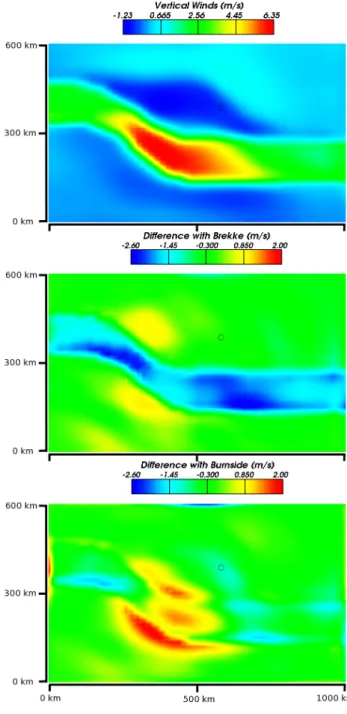
The results at three points within the modelling domain show how the vertical wind and the Burnside and Brekke condi-tions vary with time. Figures 4 and 5 show how the two conditions behave spatially at two separate times. These two figures have the following format: The vertical winds are plotted in the top panel, the middle and bottom panels are
Fig. 4. The top panel shows the vertical wind from the model at a height of 325 km after 5400 model seconds. The model extends 1000 km zonally and 600 km meridionally, the length and width of the plot respectively. The differences between the Brekke and Burnside conditions predictions and the model vertical wind (verti-cal wind less prediction) are shown in the middle and lower panels. The latitudinal and longitudinal position of the data used in Figs. 3 and 6 is represented by the circles.
plots of the vertical winds minus the Brekke and Burnside predictions respectively. Figure 4 is a slice plot at an alti-tude of 325 km after 5400 model seconds. At this stage the ion convection has been in the same place for the entirety
Fig. 5. Same format as Fig. 4 but after 5760 model seconds. The ion convection has moved to its new position and has been there for 360 model seconds. The latitudinal and longitudinal position of the data used in Figs. 3 and 6 is represented by the circles.
vertical winds speeds observed in the real atmosphere, they are at times a large percentage (up to∼40%) of the prevailing model vertical winds. The middle panel shows that although the Brekke condition winds are too large in magnitude, it does predict the correct location for these winds relative to the flow channel. The bottom panel shows the differences between the vertical winds and the Burnside condition. This plot shows that although the Burnside condition is on aver-age closer in magnitude to the model vertical wind, the dif-ferences are not as systematic as the Brekke condition. The important errors in the Brekke condition at 325 km altitude are due to an overestimation of the winds whereas the seri-ous errors in the Burnside condition are not the magnitude, but in the position and sign of the winds. Of course, these are more serious concerns.
Figure 5 presents the same quantities 360 model seconds after the ion convection has changed position, i.e., at 5760 model seconds into the simulation. These panels show the more “dynamic” forcing scenario. As before, the difference from the Brekke condition (middle panel) is larger than the Burnside condition (bottom panel) however the differences are more systematic. The Brekke winds are in the appropri-ate positions, but are overestimappropri-ated in magnitude. The Burn-side winds are quite accurate within the convection pattern, but not in some regions bordering the ion convection. This is a serious concern as it means the Burnside condition will predict vertical winds where none exist.
It must also be remembered that the Burnside condition does not perform as well at the lower heights. This can be seen in Fig. 3, showing instances where the Burnside con-dition predicts winds in the opposite direction. The results also indicate that both conditions are more accurate when the forcing has been in place for an extended period of time. 3.5 The Brekke condition overestimation problem
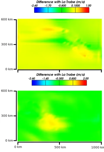
The plots show that the Brekke condition better describes the shape of the vertical wind field than the Burnside condition. The remaining concern with the Brekke condition is the ver-tical wind magnitude. It is interesting to note that at all three heights presented in Fig. 3 the Brekke condition overesti-mates the vertical winds by roughly∼67% – which is
sus-piciously similar to the factor ofγ that appears in the condi-tion. Indeed, we propose here a variation on the Brekke con-dition (that we will refer to as the “La Trobe concon-dition”) in which the adiabatic gas constantγ is simply dropped. Since the Brekke condition otherwise behaves so well spatially, it is worth considering whether there is theoretical justification for this modification.
The approximations made in deriving the Brekke condi-tion were listed earlier. The key problem for the winds stud-ied here is the assumption that vertical motion occurs adia-batically – which is obviously inappropriate for our model in which vertical winds are driven by Joule heating. It has been seen from other model runs that upwelling dampens
out quickly when the heating source is removed. This in-dicates that the upwelling can only continue if heat is con-stantly being added to the air parcel which, obviously, is not an adiabatic process. The parcels then rise at a rate such that they remain slightly positively buoyant with temperature just slightly higher than the background atmosphere at each altitude. If there is little or zero vertical temperature gradi-ent in the background atmosphere then, the rising gas parcels would represent an isothermal process rather than an adia-batic one. Rederiving the Brekke condition for an isothermal process leads to the La Trobe condition that:
uz=H∇ ·u (7)
The only difference between the Brekke condition and the La Trobe condition in their final forms is the absence of the adiabatic gas constant in the La Trobe condition.
Line plots of the La Trobe condition and vertical winds are presented in Fig. 6 which has a similar format to that of Fig. 3. This figure allows a comparison of the vertical winds (blue line) and the La Trobe condition (green line) for the en-tire time history of the model although we are going to focus on the period after 5400 model seconds. It shows that the La Trobe condition does still over estimate the vertical wind a little. Of course it retains the Brekke condition’s ability to predict the spatial structure of the model vertical wind field, because the two relations differ only by a constant. The La Trobe condition is 17% larger than the model wind at an al-titude of 225 km, 8% larger at 275 km and 13% at 325 km. Perfect agreement is of course not expected, as the actual atmosphere is not isothermal. But we do obtain a vast im-provement on the overestimations of the Brekke condition mentioned earlier.
Fig. 6. The model vertical wind is plotted (blue lines) as is the La Trobe condition predictions (green lines). As with Fig. 3 the line plots present the conditions after 5400 model seconds at altitudes of 225 km(A), 275 km(B)and 325 km(C), respectively. Again, the vertical scales are different for each plot. Circles in Figs. 4 and 5 show where data were taken from.
4 Conclusions
A local scale 3-D time dependent model has been developed to study thermospheric dynamics. Although the model has not been used to simulate a particular event it has been used to model the likely atmospheric response to a given
forc-Fig. 7. The top panel shows the difference between the vertical wind and the La Trobe condition prediction at an altitude of 325 km after 5400 model seconds. The same scale as the difference plots in Fig. 4 has been used. The bottom panel has the same format as the difference slice plots from Fig. 5 presenting the differences, after 5760 model seconds, between the model winds and the predictions using the La Trobe condition. Note that a different color scale is applied in the top and bottom panels, see text for explanation.
1. There is a relationship between divergence in the neutral wind field and vertical winds. However, it was found that the total divergence was generally a better proxy than just the horizontal divergence.
2. For this reason, the Brekke condition was able to pre-dict the correct position and direction of vertical winds, whereas the Burnside condition only predicted vertical winds of the correct sign above the height of maximum heating per unit mass (about 280 km in this case). Be-low this height, the Burnside condition predicted verti-cal winds with the opposite direction to those that actu-ally prevailed.
3. A new prediction, the La Trobe condition, retains the spatial accuracy of the Brekke condition whilst going a long way to correct the overestimation error.
4. Both the Brekke and Burnside conditions are more ac-curate under the “static” forcing regime.
5. Most importantly, this study shows that the Burnside condition is not applicable for predicting vertical winds at high latitudes below the F-Region peak, under the forcing regimes considered here. However, providing the forcing is not changing rapidly with time, it is likely to be useable above the F-region peak. Since the Burn-side condition can be evaluated from commonly avail-able experimental data, this latter result is likely the most useful practical outcome of this work.
Acknowledgements. The modelling was completed by using an open source CFD code called OpenFoam which can be obtained from http://www.opencfd.co.uk/. The models were run on a com-puter owned and operated by the Geophysical Institute, University of Alaska, Fairbanks. This research has been supported by the Aus-tralian Research Council’s Discovery Project DP0557369 and by the Australian Antarctic Science Program.
Topical Editor M. Pinnock thanks A. Aylward and J. Meriwether for their help in evaluating this paper.
References
Andr´e, R., Hanuise, C., Villain, J.-P., and Krasnoselskikh, V.: Tur-bulence characteristics inside ionospheric small-scale expanding structures observed with SuperDARN HF radars, Ann. Geophys., 21, 1839–1845, 2003,
http://www.ann-geophys.net/21/1839/2003/.
Aruliah, A. L.: The trouble with thermospheric vertical winds: geo-magnetic, seasonal and solar cycle dependence at high latitudes, J. Atmos. Terr. Phys., 57, 597–609, 1995.
Batten, S. and Rees, D.: Thermospheric winds in the auroral oval: observations of small scale structures and rapid fluctuations by a doppler imaging system, Planet. Space Sci., 38, 675–694, 1990. Biondi, A. M.: Measured vertical motion and converging and
di-verging horizontal flow of the midlatitude thermosphere, Geo-phys. Res. Lett., 11, 84–87, 1984.
Biondi, M. A., Sipler, D. P., Zipf, M. E., and Baumgardner, J. L.: All-sky doppler interferometer for thermospheric dynamics stud-ies, Appl. Optics, 34, 1646–1654, 1995.
Brekke, A.: Physics of the upper atmosphere, Praxis Publishing, 1997.
Burnside, R. G., Herrero, F. A., Meriwether Jr., J. W., and Walker, J. C. G.: Optical observations of thermospheric dynamics at Arecibo, J. Geophys. Res., 86, 5532–5540, 1981.
Chang, C. A. and St.-Maurice, J.-P.: Two-dimensional high-latitude thermospheric modeling: A comparison between moderate and extremely disturbed conditions, Can. J. Phys., 69, 1007–1031, 1991.
Conde, M. and Smith, R. W.: “Phase Compensation” of a separation scanned, all-sky imaging Fabry-Perot Spectrometer for auroral studies, Appl. Optics, 36, 5441–5450, 1997.
Conde, M. and Smith, R. W.: Spatial structure in the thermospheric horizontal wind above Poker Flat, Alaska, during solar mini-mum, J. Geophys. Res., 103, 9449–9471, 1998.
Cooper, S. L. and Conde, M.: Origins of horizontal divergence in the auroral thermosphere: A modelling study, Geophys. Res. Lett., 33, L21111, doi:10.1029/2006GL027601, 2006.
Crickmore, R. I.: A comparison between vertical winds and di-vergence in the high-latitude thermosphere, Ann. Geophys., 11, 728–733, 1993.
Crickmore, R. I., Dudeney, J. R., and Rodger, A. S.: Vertical ther-mospheric winds at the equatorward edge of the auroral oval, J. Atmos. Terr. Phys., 53, 485–492, 1991.
Deng, Y. and Ridley, A. J.: Dependence of neutral winds on convection E-field, solar EUV, and auroral particle pre-cipitation at high latitudes, J. Geophys. Res., 111, A09306, doi:10.1029/2005JA011368, 2006.
Deng, Y. and Ridley, A. J.: Possible reasons for understanding Joule heating in global models: E field variability, spatial res-olution, and vertical velocity, J. Geophys. Res., 112, A09308, doi:10.1029/2006JA012006, 2007.
Deng, Y., Richmond, A. D., Ridley, A. J., and Liu, H.-L.: Assess-ment of the non-hydrostatic effect on the upper atmosphere us-ing a general circulation model (CGM), Geophys. Res. Lett., 35, L01104, doi:10.1029/2007GL032182, 2008.
Dickinson, R. E., Ridley, E. C., and Roble, R. G.: A three-dimensional general circulation model of the thermosphere, J. Geophys. Res., 86, 1499–1512, 1981.
Dyson, P. L., Davies, T. P., Parkinson, M. L., Reeves, A. J., Richards, P. G., and Fairchild, C. E.: Thermospheric neutral winds at southern mid-latitudes: A comparison of optical and ionosonde hmF2 methods, J. Geophys. Res., 102, 27189–27196, 1997.
Fuller-Rowell, T. J.: A two-dimensional, high-resolution, nested-grid model of the thermosphere 2. Response of the thermosphere to narrow and broad electrodynamic features, J. Geophys. Res., 90, 6567–6586, 1985.
Fuller-Rowell, T. J. and Rees, D.: A three-dimensional time-dependent global model of the thermosphere, J. Atmos. Sci., 37, 2545–2567, 1980.
Greet, P. A., Innis, J. L., and Dyson, P. L.: Thermospheric vertical winds in the auroral oval/polar cap region, Ann. Geophys., 20, 1987–2001, 2002, http://www.ann-geophys.net/20/1987/2002/. Harris, M.: A new coupled atmosphere and thermosphere
photo-chemical coupling, PhD thesis, University College London, Lon-don, 2001.
Hedin, A. E.: Extension of the MSIS thermosphere model into the middle and lower atmosphere, J. Geophys. Res., 96, 1159–1172, 1991.
Hess, S. L.: Introduction to theoretical meteorology, Holt, Rinehart and Winston, 1959.
Innis, J. L., Greet, P. A., and Dyson, P. L.: Fabry-Perot spectrometer observations of the auroral oval/polar cap boundary above Maw-son, Antarctica, J. Atmos. Terr. Phys., 58, 1973–1988, 1996. Ishii, M., Oyama, S., Nozawa, S., Fujii, R., Sagawa, E., Watari, S.,
and Shinagawa, H.: Dynamics of neutral wind in the polar re-gion observed with two Fabry-Perot interferometers, Earth Plan-ets Space, 51, 833–844, 1999.
Ishii, M., Okano, S., Sagawa, E., Murayama, Y., Watari, S.-I., Conde, M., and Smith, R. W.: Development of CRL Fabry-Perot interferometers and observation of the thermosphere, Communi-cations Research Laboratory Review, 48, 155–164, 2002. Price, G. D., Smith, R. W., and Hernandez, G.: Simultaneous
mea-surements of large vertical winds in the upper and lower thermo-sphere, J. Atmos. Terr. Phys., 57, 631–643, 1995.
Rees, D. and Greenaway, A. H.: Doppler imaging system; An op-tical device for measuring vector winds. 1: General principles, Appl. Optics, 22, 1078–1083, 1983.
Rees, D., Smith, M. F., and Gordon, R.: The generation of vertical thermospheric winds and gravity waves at auroral latitudes – II. Theory and numerical modelling of vertical winds, Planet. Space Sci., 32, 685–705, 1984a.
Rees, D., Smith, R. W., Charleton, P. J., McCormac, F. G., Lloyd, N., and Steen, A.: The generation of vertical thermospheric winds and gravity waves at auroral latitudes – I. Observations of vertical winds, Planet. Space Sci., 32, 667–684, 1984b. Richmond, A. D., Ridley, E. C., and Roble, R. G.: A
thermo-sphere/ionosphere general circulation model with coupled elec-trodynamics, Geophys. Res. Lett., 19, 601–604, 1992.
Ridley, A. J., Deng, Y., and T´oth, G.: The global ionosphere-thermosphere model, J. Atmos. Solar-Terr. Phys., 68, 839–864, 2006.
Rishbeth, H., Moffett, R. J., and Bailey, G. J.: Continuity of air motion in the mid-latitude thermosphere, J. Atmos. Terr. Phys., 31, 1035–1047, 1969.
Sipler, D. P., Biondi, A. M., and Zipf, M. E.: Vertical winds in the midlatitude thermosphere from Fabry-Perot interferometer mea-surements, J. Atmos. Terr. Phys., 57, 621–629, 1995.
Smith, R. W.: Vertical winds: A tutorial, J. Atmos. Solar-Terr. Phys., 60, 1425–1434, 1998.
Smith, R. W. and Hernandez, G.: Vertical winds in the thermo-sphere within the polar cap, J. Atmos. Terr. Phys., 57, 611–620, 1995.
Sun, Z.-P., Turco, R. P., Walterscheid, R. L., Venkateswaran, V., and Jones, P. W.: Thermospheric response to morningside dif-fuse aurora: High-resolution three-dimensional simulations, J. Geophys. Res., 100, 23779–23793, 1995.
Thayer, J. P. and Killeen, T. L.: A kinematic analysis of the high-latitude thermospheric circulation pattern, J. Geophys. Res., 98, 11549–11565, 1993.
Walterscheid, R. L. and Lyons, L. R.: The neutral circulation in the vicinity of a stable auroral arc, J. Geophys. Res., 97, 19489– 19499, 1992.
Walterscheid, R. L., Lyons, L. R., and Taylor, K. E.: The perturbed neutral circulation in the vicinity of a symmetric stable auroral arc, J. Geophys. Res., 90, 12235–12248, 1985.
Wang, W., Killeen, T. L., Burns, A. G., and Roble, R. G.: A high-resolution, three-dimensional, time dependent, nested grid model of the coupled thermosphere-ionosphere, J. Atmos. Solar-Terr. Phys., 61, 385–397, 1999.