Comput. Appl. Math. vol.25 número1

ISSN 0101-8205 www.scielo.br/cam

Wave sequences for solid fuel adiabatic in-situ

combustion in porous media

A.J. DE SOUZA1, I.Y. AKKUTLU2 and D. MARCHESIN3 1_{Departamento de Matemática e Estatística, Universidade Federal de Campina Grande}

Av. Aprigio Veloso, 882, 58109-970 Campina Grande, PB, Brazil

2_{Department of Civil and Environmental Engineering}

University of Alberta, Edmonton, Canada, T6G 2W2

3_{Instituto Nacional de Matemática Pura e Aplicada, Estrada Dona Castorina, 110}

Jardim Botânico, 22460-320 Rio de Janeiro, RJ, Brazil

Emails: [email protected] / [email protected] / [email protected]

Abstract. We study the Riemann problem with forward combustion due to injection of air into a porous medium containing solid fuel. We neglect air compressibility and heat loss to the rock formation. Given initial reservoir and injection conditions, we prove that there is a unique time asymptotic wave sequence for combustion with complete oxygen consumption. The sequence consists of a region of unburned air at injection temperature, a warming discontinuity, a hot region with unburned air, a combustion wave and a region with burned air and unburned fuel at the initial reservoir temperature. The waves have very different speeds, and therefore they cannot be detected in laboratory experiments that focus on the combustion wave. However, they should occur in field scale.

By introducing a cut-off in Arrhenius’ law, the reaction rate vanishes at reservoir temperature, and two types of wave sequences are possible. One was already described. The other occurs for incomplete oxygen consumption. In this case, the wave sequence contains another wave, i.e., there is another region ahead of the combustion wave containing incompletely burned air at reservoir temperature, and a gas composition discontinuity that moves fast. However, instead of a unique solution for each Riemann data, there is a one parameter family of wave speeds and strengths. This multiplicity of solutions may to be due to the cut-off.

Mathematical subject classification: 80A25, 76S05.

Key words: coflow filtration combustion, porous media, Riemann solution.

1 Introduction

Air injection and in-situ combustion have long been considered as a potential technique for displacement and recovery of heavy oil reserves [7, 22]. Opera-tional advantage of this thermal recovery technique is the abundance of injection gas independently of location. It utilizes heavy and immobile components of the crude oil as fuel producing in-place heat necessary for the recovery of upgraded crude oil.

Despite the advantages and a long history, only a small fraction of the total thermal recovery utilizes this technique. Some reasons are technical, such as the possibility of front extinction and the necessity of (re-)ignition for sustained propagation within in-situ combustion in the presence of external heat losses [1]. Thus mathematical analysis of this problem is important to predict these events. A large number of studies on the structure of the combustion front have been reported since 1950s, see [1, 2, 3, 4, 5, 6, 8, 20, 21, 23, 26], for instance. These studies did not take into account other waves that occur in the combustion problem. As there is interaction between the combustion wave and other waves, this paper focuses on the solution of the Riemann problem with combustion taking into account all possible waves.

The paper is subdivided as follows. In Section 2 we present the mathematical model. Theory on systems of conservation laws suggests that, besides the com-bustion front, there could be rarefaction, shock or contact waves. In Section 3 we determine the characteristic speeds and prove that in this model there are neither rarefaction nor shock waves, only contact discontinuities. In fact, an examination of the Rankine-Hugoniot conditions shows that all noncombustion discontinuities are just the contact waves already found. In Section 4 we intro-duce the combustion front as a traveling wave of the evolution system derived in Section 2. In this section we also discuss the Rankine-Hugoniot jump conditions for the combustion wave. In Section 5 we prove that for the physical parameters considered in this paper, there are no resonances between waves, as opposed to the case analyzed by Aldushin et al. in [4]. As a consequence of the absence of resonances, we obtain two distinct temperature relationships for the combustion front, which we call thehot upstreamand thehot downstreamcombustion cases. In Section 6 we determine the ranges of parameters in which these combustion waves may exist. In Section 7 we present our main results. For the hot upstream combustion we prove in Theorem 7.1 that the wave sequence of the Riemann solution is uniquely determined in case of complete consumption of oxygen. In Theorem 7.2 we prove that, for incomplete consumption of oxygen (using a modified version of the Arrhenius’ law), there is another wave sequence as a solution. However, this solution is not unique, rather it is a one-parameter fam-ily of solutions. We also show that the hot downstream case does not occur in this model. In Appendix A we present tables with typical values of parameters, constants and nomenclature used through the paper.

2 Formulation of the problem

We assume that air is injected at the leftmost part of a porous rock cylinder containing solid fuel, so that all wave propagation is one dimensional. Balance equations are written for the total energy, the total gas mass, the oxygen mass and the fuel mass. For the latter, we define the fuel density per total volumeρf and

introduce the extent of conversion depth,η(x˜,t˜)=1−ρf(x˜,t˜)/ρof (ρ o

f is the

latter may occur because the fuel was never present or because it was completely consumed). The primary dependent variables are the temperature,T˜(x˜,t˜), the oxygen concentration in terms of mass fraction,Y˜(x˜,t˜)and the fuel conversion depthη(x˜,t˜). The gas densityρg(T˜,p˜)is expressed by the ideal gas equation

of state in terms of temperature and total gas pressure p˜(x˜,t˜).

In formulating the conservation equations we make the following assump-tions: the pore space and the solid matrix are in thermal equilibrium so that a one-temperature model is used for the energy balance; heat transfer by radiation, energy source terms due to pressure increase, and work from surface and body forces are all negligible; the ideal gas law is the equation of state for the gas phase; thermodynamic and transport properties, such as conductivity, diffusiv-ity, heat capacity of the solid, heat of reaction, etc., all remain constant. We also neglect heat loss to the surrounding rock formation. We assume that gas heat capacity is negligible with respect to the rock heat capacity. The heat loss will be taken as zero as we study only the adiabatic case in this work. We assume that the pressure changes within any wave are negligible compared to the pres-sure drop across the system, so that in the ideal gas law and in other physical properties the pressure appears as a constant. Under these assumptions the di-mensional form (indicated by the superscript tilde) of the energy balance, the oxy-gen mass balance, the gaseous phase mass balance and the combustion kinetics equations are:

(1−φ)∂(csρs ˜

T) ∂t˜ +

∂(cgρgv˜T˜) ∂x˜ = ˜λ

∂2_T˜ ∂x˜2 +Qρ

o

fW, (2.1)

φ∂(ρg ˜

Y) ∂t˜ +

∂(ρgv˜Y˜) ∂x˜ =DM

∂ ∂x˜

ρg ∂Y˜

∂x˜

− ˜µρo_fW, (2.2)

φ∂(ρg) ∂t˜ +

∂ρgv˜

∂x˜ = ˜µgρ o

fW, (2.3)

∂η

∂t˜ =W, (2.4)

rate of the gas phase. In the above,ci denotes the average specific heat capacity

of speciesi (gas or solid) at constant pressure,ρi is the volumetric density of

speciesi,λ˜ is the effective thermal conductivity (λ˜s=λ˜g),Qis the heat released

due to reaction (per unit mass of solid). Changes in the porosityφare considered to be negligible so that φ is constant. DM is an effective diffusion coefficient

in the gas phase (D=DM/φ, where D is the molecular diffusion coefficient),

whileµ˜ = ˜γMo/Mf andµ˜gp = ˜γgpMgp/Mf are mass-weighted stoichiometric

coefficients for oxygen and for combustion gaseous products, respectively. Mo,

Mf and Mgp are the molecular weight of oxygen, fuel and gaseous products,

respectively. The net gas mass production is determined fromµ˜g = ˜µgp − ˜µ,

so that positive or negative sign for µ˜g correspond to net gaseous phase mass

production or consumption, respectively. We will assumeµ˜g >0. For the rate

of reaction, we use the second order law of mass action and the Arrhenius’ Law:

W =k0e−E/R ˜

T_{Y˜(1−η) , (2.5)}

with activation energy Eand pre-exponential factorko.

We use the ideal gas equation of statep M˜ g =ρgRT˜, whereRis the universal

gas constant, whileMgandρgare the effective molecular weight and the effective

density of the gas phase, respectively. We neglect the effect of changes of Mg

due to the reaction by approximating Mgby a constant.

Non-dimensionalized combustion equations. We introduce dimensionless space and time variables. To bring out the internal structure of the combus-tion wave, we introduce convenient variables and parameters that are defined in Appendix A. We scale the length byl∗=αs/vi and the time usingt∗=l∗/vi, where vi_{is the injection velocity andα}

s the effective thermal diffusivity. We introduce

the scaled temperatureθ = ˜T/T˜0, which means that the reservoir temperature

corresponds toθ0 = 1; we also introduce the nondimensional gas density ρ,

which is the gas density divided by the gas density at reservoir temperature. Thus the equations (2.1)–(2.4) are transformed into four dimensionless balance equations (2.6)–(2.9), while the dimensionless ideal gas law becomes Eq. (2.10):

∂θ ∂tˆ +

∂(aρvθ ) ∂xˆ =

∂2_θ

∂(φYρ) ∂tˆ +

∂(ρvY) ∂xˆ =

1 Le

∂ ∂xˆ

ρ∂Y ∂xˆ

−µ , (2.7)

φ∂ρ ∂tˆ +

∂(ρv)

∂xˆ =µg , (2.8)

∂η

∂tˆ = , (2.9)

ρθ =1, (2.10)

where

=αe−γ /θY(1−η) . (2.11)

The domain of the dependent variables is given by

θ >0, 0≤Y ≤1, 0≤η≤1, v >0. (2.12)

From now on, we writetˆ→t,xˆ →x.

The values of the parametersa,q,φ,Le,µ,µg,α andγ are given in Table 1

of Appendix A.

3 Non-combustion waves for the model in hyperbolic framework

In the absence of combustion, the source terms representing mass transfer or sensible heat generation containing the factor vanish on the right hand sides of system (2.6)–(2.10). Of course vanishes forY ≡ 0 orη ≡ 1. We focus in the waves for large times and long distances for which the second derivative terms are negligible. Let us first consider smooth solutions, so we can expand the derivatives in the remaining terms in Eqs. (2.6-2.9), manipulate Eqs. (2.7), (2.8), use Eq. (2.10) to eliminateρ, obtaining:

∂θ ∂t +a

∂v

∂x =0, (3.1)

φ∂Y ∂t +v

∂Y

∂x =0, (3.2)

θ

a +φ

∂θ ∂t +v

∂θ

∂η

∂t =0. (3.4)

The characteristic speeds of system (3.1)–(3.4) in increasing order and the corresponding characteristic vectors are:

λη =0, (0,0,1,0)T, (3.5)

λθ =a v

θ+aφ,

1,0,0, v θ +aφ

T

, (3.6)

λY = v

φ, (0,1,0,0)

T_{. (3.7)}

It is easy to see that all characteristic speeds are constant along the integral curves defined by the corresponding characteristic vector fields, which means that all of them are associated to contact discontinuities, hence they satisfy the Rankine-Hugoniot conditions for (3.1)–(3.4), [25]. The characteristic speedλη corresponds to an immobile discontinuity along which onlyηvaries,λθ corre-sponds to a thermal discontinuity along whichθ andvvary andλY corresponds to a gas composition discontinuity along which onlyY varies.

4 The combustion wave

We proceed next with the study of combustion wave propagation. The combus-tion wave encountersunburned statesahead and leavesburned statesbehind it. We look for combustion fronts as steady traveling waves of system (2.6)–(2.11) with propagation speedV >0 by settingx = ˆx−Vtˆandt = ˆt. In these moving nondimensional coordinates, after using Eq. (2.10) to eliminateρ, the equations (2.6)–(2.9) read, after writingxˆ →x:

d

d x (av−Vθ )= d2_θ

d x2 −q

d(Vη)

d x , (4.1)

d d x

1

θ(v−φV)Y

= 1

Le

d d x

1 θ

dY d x

+µd(Vη)

d x , (4.2)

d d x

1

θ(v−φV)

= −µg

d(Vη)

d(Vη)

d x = − . (4.4)

In the adiabatic case studied here, reaction at the back of the combustion zone ceases due to complete lack of fuel, i.e., ηb=1 at −∞. This is fuel-deficient combustion. (Thus, there can be no second combustion wave behind the first one.) Since gas is injected we haveYb _{= 1. The temperature and the velocity}

behind the combustion need to be calculated. Thus the boundary conditions behind this combustion front are generically given by:

θ =θb>0, Y =Yb =1, η=ηb=1, v=vb>0; x → −∞, (4.5)

where the superscriptbmeansburned.

Ahead of the combustion zone we consider that there is abundant fuel, i.e., ηu=0 at+∞, under two distinct conditions surrounding the combustion front. The first condition is thecomplete oxygen consumption casewhere we setYu₌₀

at +∞. The second condition is the temperature-controlled case where we set θu = 1 at+∞, andYu _{have to be determined. The study of this second}

case is of special interest in petroleum applications, as it represents a situation where oxigen advances faster than the combustion wave, and the breakthrough of oxigen at the producing well causes safety hazards and other operational difficulties. These conditions can be summarized in (4.6) and (4.7), respectively:

θ =θu >0, Y =Yu=0, η=ηu =0, v=vu >0; x → +∞, (4.6)

θ =θu =1, Y =Yu >0, η=ηu =0, v=vu >0; x → +∞. (4.7)

where the superscriptumeansunburned.

Integrating equations (4.1)–(4.3) fromxto+∞once, taking into account that ηu _{=0 atx = +∞and re-ordering, we get:}

dθ

d x =a(v−v

u_{)−V(θ −θ}u_{)+qη, (4.8)}

dY d x =Leθ

1

θ(v−φV)Y − 1 θu(v

u_−φV)Yu_−µVη

, (4.9)

1

θ(v−φV)− 1 θu(v

u₋

Vdη

d x = − . (4.11)

Next, we substitute the value ofvgiven by equation (4.10) into (4.8) and (4.9), and substitute the value of given by Eq. (2.11) into (4.11) to obtain the reduced system:

dθ

d x =a

vuθ θu −

θ θu −1

φ+µgηθ

V −vu

−V(θ−θu−qη), (4.12)

dY d x =Leθ

vu θu −

φ

θu +µgη

V

Y −µVη− 1 θu

vu−φVYu

, (4.13)

dη

d x = −

α

VY(1−η)e

−γ /θ_{. (4.14)}

We warn the reader that the temperature-dependent exponential on the right hand side of equation (4.14) will be modified when the temperature-controlled case given by the boundary condition (4.7) is studied.

The existence of solutions of system (4.12)–(4.14) for the boundary conditions (4.5) and (4.6), or (4.7), connecting the burned stateUb ≡ (θb,Yb, ηb;vb)at x → −∞to the unburned stateUu_≡(θu_,Yu_{, η}u_;vu_{)andx → +∞is studied}

in a separate work, [9, 10]. Such solution represents the profile of a traveling wave connecting the burned state to the unburned state. For large times, this traveling wave is regarded as a thin combustion shock, [11, 15]. The Rankine-Hugoniot condition relating the burned and unburned states is studied in the next subsection.

4.1 The Rankine-Hugoniot equations for the combustion wave

For the boundary conditions given in (4.5) at−∞and in (4.6), or (4.7), at+∞, taking into account that∂θ/∂x, ∂Y/∂x and∂η/∂x tend to zero as x tends to

±∞, the R.H.S. of equations (4.12)–(4.13) become:

a

vuθb θu −

θb θu −1

φ+µgθb

V −vu

−V(θb−θu−q)=0, (4.15)

Leθb

vu θu −

φ

θu +µ+µg

V − 1 θu(v

u_−φV)Yu

and Eq. (4.14) becomes a trivial identity. Taking x → −∞in Eq. (4.10) we obtain a separate equation forvb:

vb−φV =

1 θu(v

u_−φV)−µ gV

θb. (4.17)

The solutions of the Rankine-Hugoniot equations (4.15)–(4.17) together with the equation =0 determine all pairs of left and right states that are equilibria of system (4.12)–(4.14), i.e., that have the potential of representing burned and unburned states associated to a combustion wave.

4.2 Geometric analysis of the Rankine-Hugoniot equations

Since λY _{is the particle speed of gas it is convenient to introduce the scaled}

combustion wave speedVu(V, vu)≡V/λY(Uu)given by:

Vu = φV

vu . (4.18)

Here the superscriptuinVu_{reminds the reader thatV was scaled byv}u_.

Equa-tions (4.15) and (4.16) giveθbandYu in terms ofV,vu andθu, or in terms of Vu_andθu_{as follows:}

θb = ((θ

u_{+q+aφ)V −av}u_{) θ}u

(1+aµg)θu+aφ

V −avu , or

θb = ((θ

u_+q+aφ)Vu_{−aφ) θ}u

(1+aµg)θu+aφ

Vu_−aφ,

(4.19)

Yu = v u₋

φ+(µg+µ)θu

V

vu_−φV , or

Yu = φ−

φ+(µg+µ)θu

Vu

φ(1−Vu₎ .

(4.20)

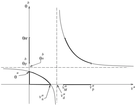
For a fixed value ofθu, Eq. (4.19b) representsθbin terms ofVuas a hyperbola drawn schematically in Fig. 4.1, constructed for parameter values given in Ap-pendix A. The hyperbola has vertical and horizontal asymptotes respectively at:

V_du = aφ

(1+aµg)θu+aφ

, θ_ab= (θ

u_+q+aφ)θu

(1+aµg)θu+aφ

d θ

θ

a

n p

θ

p θM

θ

M u

b

b

b

Vu V

u

Vu

Vu Vu

Figure 4.1 –θbas a function ofVu_{given by (4.19b).}

The intersections of this hyperbola with the horizontal and vertical coordinate axes occur at:

θb=θu, and V_nu= aφ

θu_+q+aφ. (4.22)

Since aµg < q notice that Eqs. (4.21) and (4.22) lead toθab > θ

u _andVu n <

V_du <1, respectively.

Remark 4.1. The constants Vu

p andθbp = θb(Vpu) in Fig. 4.2 are related to

Eq. (4.20b) and will be explained in the text. The constant θM is defined by

Eq. (5.1) andV_Mu =Vu_(θ

M)is obtained from (4.27).

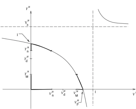
Now let us consider Eq. (4.20b) for a fixed value ofθu. This equation represents Yu_{in terms ofV}u_{as another hyperbola, which is drawn schematically in Fig. 4.2.}

This hyperbola has vertical asymptote Vu = 1 and horizontal asymptote at Yu

a = φ+θu(µ+µg)/φ, which has no physical meaning; see the horizontal

1 Y

Y_a

1

p d Y

d

Y

n Y

n

M M

u

u

u

u

u

Vu Vu Vu Vu

Vu

Figure 4.2 –Yuas a function ofVugiven by (4.20b).

The intersections of this hyperbola with the horizontal and vertical coordinate axes occur at:

V_pu= φ

φ+(µ+µg)θu

and Yu=1. (4.23)

Knowing the value ofV_puwe define the scaled temperature value:

θ_pb=θb(V_pu), where the expression ofθbis defined in Eq. (4.19b). (4.24)

Notice thatV_pu =1/Y_au<1.

Remark 4.2. For the quantities in Fig. 4.1 and 4.2, corresponding to the pa-rameters in Table 1, the inequalities 0<V_nu <V_du <V_Mu <V_pu <1 hold.

We have expressedθbandYu in terms ofVu. Now, let us also expressθbin terms of the scaled combustion speed:

here the superscriptbinVb_{reminds the reader thatV was scaled byv}b_.

Using Eq. (4.17) we obtain:

vu= 1 θb

θuvb+

(θb−θu)φ+µgθuθb

V

. (4.26)

Alternatively, instead of obtaining an expression forθbas a function ofVu_and θuas in (4.19b), Eq. (4.15) could be utilized to findVuas function ofθbandθu:

Vu= aφ (θ

u_−θb₎

(θu₎2₋

(θb_{−q)−a(φ−µ} gθb)

θu_−aφθb . (4.27)

SimilarlyVbcan be written in terms ofθb:

Vb= aφ(θ

b_−θu₎

(θb₎2₋

(θu_{+q)−a(φ+µ} gθu)

θb_−aφθu. (4.28)

θ2 θ

1

θp p

θ1 θ θM

M

b 0 u b b b

Vb Vb

Vb

Figure 4.3 –Vb θb

defined by equation (4.28).

Fig. 4.3 shows schematically Vb_(θb_{). The denominator in Eq. (4.28) is}

θb _{= θ}b

1 andθb = θ b

2. The graph possesses also a horizontal asymptote given

byVb =0.

We recall that we are interested in forward combustion, so we restrict our attention to the caseV >0. From Eqs. (4.18) and (4.25) it follows thatVu>0 and Vb _{> 0. Thus, only the portions in the first quadrant of the graphs in}

Figs. 4.1, 4.2 and 4.3 are considered.

We conclude that the geometric analysis performed in this section yields the following restrictions relating burned and unburned states:

0<Vu<V_nu, or V_du <Vu≤ V_pu, (4.29)

0≤θb< θu, or θb≥θb_p> θu, (4.30)

0<Vb<1, (4.31)

where Vu_{, V}u

d, Vnu, Vpu,θbp and Vb are defined by equations in (4.18), (4.21),

(4.22), (4.23), (4.24) and (4.25), respectively.

5 Wave resonances

We can expect that changes of wave structure in the combustion Riemann pro-blem occur whenever two wave speeds coincide, either in the burned or in the unburned regions. In this way we could have an interchange of the relative position of two waves. For the parameter values in Table 1 such changes are ruled out for physically interesting temperature range by the following theorem about absence of resonances:

Theorem 5.1. LetθM be defined by

θM =

q aµg

. (5.1)

Then in the physical domain defined by Eq.(2.12):

(a) the non-combustion waves have distinct speeds;

(c) consider a combustion wave following a thermal wave, i.e., V < λθ_(Uu_).

In the limit as they tend to have equal speed, the temperature at the left of the superposed waves isθb_=θ

M.

(d) consider a thermal wave following a combustion wave, i.e.,λθ_(Ub_{) <V .}

In the limit as they tend to have equal speed, the temperature at the right of the superposed waves isθu _=θ

M.

Proof.

(a) From equations (3.5)–(3.7) we obtain explicitly that

λη < λθ < λY everywhere, (5.2)

which means that there are no speed equalities among non-combustion waves.

(b) Since we are considering forward combustion there is no resonance bet-ween the combustion and the immobile wave.

From Eqs. (4.29) and (4.31), we have that 0<Vu _{<1 and 0<V}b _<1,

respectively. Since Vu = V/λY(Uu) and Vb = V/λY(Ub), it follows respectively that

V < λY(Uu) andV < λY(Ub) . (5.3)

(c) From Eqs. (3.6), (4.18) and (4.27), the combustion wave following a ther-mal wave tend to have the same speed if, and only if,Vu =aφ/ (θu+aφ), or

(θu−θb)

(θu₎2₋

(θb_{−q)−a(φ−µ}

gθb)θu−aφθb

= 1

θu_+aφ, or

θu(aµgθb−q) = 0 or θb = θM.

(5.4)

Direct calculations with the value of the parameters in Table 1 yield θM ≈

24.21264641. This corresponds to an extremely large temperature value above 6000 K that is beyond physical interest in our case; even at temperatures lower than 6000 K we may expect that heat losses to the surrounding reservoir can-not be neglected. This valueθM defines a maximum temperature value, below

which there are no speed coincidences. Thus we focus our attention to the tem-perature range 0< θ ≪θM.

So one conclusion of this section is that for physical values of temperature there are no resonances between waves in this model.

Remark 5.2. The case where the thermal wave speed coincides with the com-bustion wave speed yields high temperatures and therefore maximal comcom-bustion efficiency. It is called superadiabatic combustion, which is desirable in other practical applications. The structure of such a combustion wave was analyzed in [4].

Since Vu _{and V}b _{are both positive, by analyzing the first denominator in}

Eq. (5.4) one can see that the sign of(θb−θu)determines ifV < λθ _{orV > λ}θ_. Thus, our final conclusion in this section is that the following two temperature relationships for the combustion front are possible:

(A) Hot upstream (left)

θb> θu >0, for V > λθ(Ub) and V > λθ(Uu); (5.5)

(B) Hot downstream (right)

0< θb < θu, for V < λθ(Ub) and V < λθ(Uu) . (5.6)

6 The admissible Rankine-Hugoniot locus for the combustion wave

Cases (A) and (B) in (5.5) and (5.6) yield distinct possibilities for the ranges of θb_{, V}b_{, V}u _{and Y}u _{corresponding to distinct portions of the branches in}

Figs. 4.1, 4.2 and 4.3. Such ranges are called the admissible states for combustion waves. In the next two subsections we will obtain the admissible ranges, which are fully characterized by the value ofVu: the first one is V_Mu < Vu ≤ V_puand the second one is 0<Vu_≤Vu

6.1 Hot upstream

Since θb > θu (see Fig. 4.1) it follows that Vu > V_du. As 0 ≤ Yb ≤ 1 (see Fig. 4.2) it follows thatVu_{≤ V}u

p.

Let us define

V_Mu =Vu(θM) , (6.1)

represented in Fig. 4.1 and obtained from Eq. (4.27), whereθM is the maximum

value for the nondimensionalized temperatureθ defined in (5.1). Let us also define

V_Mb =Vb(θM) , and Vpb =V b

(θb_p) , (6.2)

represented in Fig. 4.3, where the expressionVbis defined in Eq. (4.28). Finally, letYu

M in Fig. 4.2 be defined as

Y_Mu =Yu(V_Mu), where the expression forYuis defined in Eq. (4.20b). (6.3)

By comparing the graphs in Figs. 4.1, 4.2 and 4.3, and taking into account the inequalities obtained through the previous sections we arrive at the following Lemma, which characterizes the admissible Hugoniot locus for hot upstream combustion waves:

Lemma 6.1. Let θu be a fixed value of the scaled temperature in the range 0< θu _{< θ}

M. Then the inequalities

V_Mu <Vu ≤V_pu,

(see Figs. 4.1, 4.2 and definitions in (6.1), (4.18), (4.23)), (6.4)

hold if, and only if all of the following inequalities hold:

θ_pb ≤ θb< θM, (see Figs. 4.1, 4.3 and definitions in (4.24), (5.1)); (6.5)

0 ≤ Yu <Y_Mu , (see Fig. 4.2 and definition in (6.3)); (6.6)

VMb <V b _≤

Vpb, (see Fig. 4.3 and definitions in (6.2) and (4.25)). (6.7)

6.2 Hot downstream

Since 0< θb < θuwe see that 0 <Vu ≤ V_nu, where V_nuwas defined in (4.22). See Fig. 4.1. LetYu

n in Fig. 4.2 be defined as

Y_nu = Yu(V_nu) , (6.8)

where the functionYu_{is defined by Eq. (4.20b).}

As 0 < Vu ≤ V_nu and 0 ≤ θb < θu it follows that Y_nu ≤ Yu < 1 and 0<Vb_{≤1. See Figs. 4.2 and 4.3, respectively.}

As in the previous case, by comparing the graphs in Figs. 4.1, 4.2 and 4.3, and taking into account the inequalities obtained throughout the previous sections we arrive at the following Lemma, which characterizes the admissible Hugoniot locus for hot downstream combustion waves:

Lemma 6.2. Let θu _{be a fixed value of the scaled temperature in the range}

0< θu < θM. Then the inequalities

0<Vu ≤V_nu,

(see Figs. 4.1, 4.2 and definitions in (4.18) and (4.22)), (6.9)

hold if, and only if all of the following inequalities hold:

0 < θb < θu, (see Figs. 4.1, 4.3), (6.10)

Y_nu ≤ Yu < 1, (see Fig. 4.2 and definition in (6.8)), (6.11)

0 < Vb < 1, (see Fig. 4.3 and definition in (4.25)). (6.12)

7 Wave sequences in the Riemann solutions

describe the wave sequence in the Riemann solution under the conditions (4.6) and (4.7) surrounding the combustion front, where the waves satisfy an extension of Lax speed inequalities.

7.1 Hot upstream combustion case

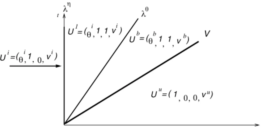
In the hot upstream combustion case the thermal wave precedes the combustion wave (λθ(Ub) < V), there is no temperature change ahead the combustion wave, which means thatθu =1 (reservoir temperature) andθb> θu =1. Thus, generically the wave sequence in the Riemann solution consists of a (perhaps trivial) immobile fuel shock, a thermal shock with speedλθ, a combustion front with speedV and a gas composition wave with speedλY_{. We denote this}

se-quence of waves by means of the following convention:

Ui λ

η

−→U1 λ

θ

−→Ub−→V Uu λ Y

−→U0. (7.1)

The stateUi _=(θi_{,1,0, v}i_{)denotes the injection conditions,U}1_=(θi_{,1,1, v}i₎

denotes an intermediate state in the burned region, while Ub = (θb,1,1, vb) andUu = (1,Yu,0, vu) are the burned and the unburned states surrounding the combustion front and U0 _{= (1,0,0, v}0_{) denotes the reservoir conditions}

at production. The values of θi andvi are given as boundary conditions, the values ofθu_andYu_{are given by condition (4.6) or (4.7), but the speedsλ}θ_,V, λY and the values ofθb,vb,vuandv0have to be determined.

7.1.1 The hot upstream combustion in the oxygen deficient case

As discussed above, we have thatθu =1 and according to the condition (4.6), which characterizes the oxygen deficient case,Yu =0. We have the following theorem, which provides formulae for all the states as well as speeds for com-bustion and noncomcom-bustion waves in the wave sequence (7.1) for the Riemann solution in this case:

Ui _{= (θ}i_{, 1, 0, v}i_{), withθ}i _{> 0andv}i _{> 0, then the constant states and the}

speeds of all waves in the wave sequence(7.1)are uniquely determined.

Proof. Inspecting Fig. 7.1 we see that the speeds and the intermediate states in the wave sequence (7.1) are determined as follows.

SubstitutingYu _{=0 in Eq. (4.20b) it follows thatV}u_=Vu

p, whereVpuis given

in (4.23) withθu _{= 1 (see Figs. 4.1 and 4.2). From Eq. (3.6) and Eq. (4.19b)}

withθu =1 andVu =Vpu, it follows that:

λθ = av i

θi_+aφ and θ

b₌ 1+q−a(µ+µg)

1−aµ .

Taking into account that the thermal wave is a contact discontinuity and Eq. (4.28) withθu =1 it follows that:

vb= θ b_+aφ

θi _+aφ v

i _{and V}b₌ aφ (θ

b₋₁₎

(θb₎2₋

1+q−a(φ+µg)

θb_−aφ.

From Eq. (4.25) we obtain the combustion speedV; then we obtainvu _from

Eq. (4.18):

V = v b_Vb

φ , v

u₌ φV

Vu .

SinceYu _{=0, the strength of the gas composition wave is zero, which explains}

why this wave is discarded in the wave sequence (7.1) as represented in Fig 7.1. Thus the proof of Theorem 7.1 is complete.

7.1.2 The hot upstream combustion in the temperature-controlled case

According to condition (4.7) we haveθu_{=1, butY}u_{have to be obtained.}

First of all we notice that the condition (4.7) cannot be analyzed as (4.6) since the unburned state Uu is not an equilibrium of system (4.12)–(4.14), because does not vanish. However the exponential factor in (2.5) is extremely small at prevailing temperatures, so we use the following modified version of the Arrhenius’ law, [27]:

W(T˜)=k0e−E

b_/(R(T˜_{− ˜T}

0))_Y˜_{(1−η) , for T}˜ _>T˜

0, and

W(T˜)=0, for T˜ ≤ ˜T0,

V

x t

(_{θ ,}i1_{, ,0} vi) Ui=

η

θ

b

θb_{, , ,}1 1 _vb

( ₎

(_{θ ,}i1_{, ,}1 vi) U =1

U =

(1_{, 0 0, ,}v ) =

Uu u

λ λ

Figure 7.1 – Regions separated by immobile, thermal wave and combustion waves in the Riemann solution. Values ofθ,Y,ηandvin each region.

whereEb=E(T˜b− ˜T0)/T˜b.

This modification on the denominator in the exponential factor ensures that the reaction rate is equal to zero below the reservoir temperatureT˜0, which is a

good approximation of the original formula in the Arrhenius’ law. The value of Ebis chosen so that at the burned state above reservoir temperature the exponent assumes the same values as in the original Arrhenius’ formula. Thus in the scaled temperature variable the function in (2.11) is replaced by the approximation

=αe−γ (1−1/θ b₎

θ−1 _Y(1−_{η) , for θ >1 and} =_{0 for θ} ≤_1.

With the above modified version of Arrhenius’ law, the unburned state Uu becomes an equilibrium of system (4.12)–(4.14) and the existence of traveling wave solutions can be obtained, [9].

Now we notice that sinceθu=1 the range forVuin Eq. (6.4) can be restricted further to

V_Mu ≤Vu ≤V₁u, where V₁u= φ φ+µ+µg

(7.3)

is obtained from Eq. (4.23) withθu _{=1. Consequently we get}

θ₁b≤θb≤θM, 0≤Yu <YMu , V b M ≤V

b_{≤ V}b 1 ,

We can prove the following theorem in this case:

Theorem 7.2. Assume that in the wave sequence for the Riemann solution of

(2.6)-(2.11)there is a hot upstream combustion wave governed by version(7.2)

of Arrhenius’ law with left and right states satisfying conditions(4.5)and(4.7), andθb _{> θ}u _{= 1. Given the injection conditions U}i _{= (θ}i_{, 1, 0, v}i_{), with} θi >0,vi >0and any positive value of the scaled combustion wave speed Vu in the interval[Vu

M, V1u]given in(7.3), then all the constant states and speeds

of all waves in the wave sequence(7.1)is uniquely determined.

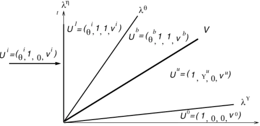
Proof. Inspecting Fig. 7.2, we see that if the injection ratevi, the temperature θi _{and the value of V}u _{are given, then the speedsλ}θ_{, V andλ}Y _{as well as the}

values ofθb,vb,Yu,vuandv0are determined as follows. From Eq. (3.6) and Eq. (4.19) withθu_{=1, we have:}

λθ = av i

θi _+aφ and θ

b₌ (1+q +aφ)Vu−aφ

1+aµg+aφ

Vu_−aφ .

Taking into account that the thermal wave is a contact discontinuity and Eq. (4.28) withθu =1 it follows that:

vb = θ b_+aφ

θi _+aφ v

i _{and V}b₌ aφ (θ

b₋₁₎

(θb₎2₋

(1+q)−a(φ+µg)

θb_−aφ.

From Eq. (4.25) we obtain the combustion speed V; then we obtain vu from Eq. (4.18). From Eq. (4.20b) withθu_{=1, we obtainY}u_{and from Eq. (3.7) with} v=vu, we obtain the value ofλY:

V = v b_Vb

φ , v

u ₌ φV

Vu , Y

u ₌ φ−

φ+µg+µ

Vu

φ (1−Vu₎ , λ Y ₌ v

u

φ .

V

( _{, 0 0, ,}v )

b

θ

Y

θb_{, , ,}1 1 _vb

( ₎

1_{, , ,}v

( Yu )

x t

(_{θ ,}i1_{, ,}1vi)

0

1 U =1

η

U =

U =u

U =0 0

(_{θ ,}i1_{, ,0} vi) Ui=

u

λ

λ _λ

Figure 7.2 – Regions separated by immobile, thermal, combustion and gas composition waves in the Riemann solution. Values ofθ,Y,ηandvin each region. The latter region is actually very thin.

Remark 7.3. We notice that, due to the fact that the combustion and the ther-mal waves are very slow, it takes a long time for these waves to separate from each other, while the gas composition wave (the extremely fast wave) separates from the others immediately. This should explain why such phenomena have not been detected in laboratory experiments, where transient rather than asymp-totic behavior is detected.

Remark 7.4. As we have seen in Theorem 7.2, in this case the injection con-ditions together with the initial data are not sufficient to determine the Riemann solution uniquely, but they determine a family of Riemann solutions depending on the parameter Vu. This strange multiplicity of solutions for the Riemann problem may to be related to the modification of the exponential factor (7.2) in Arrhenius’ law.

7.2 Hot downstream combustion

Recall that in the hot downstream combustion case we have to restrict the pa-rameters to the ranges defined by Eqs. (6.9)–(6.12). Since 0 < Yu

n < Yu < 1

the complete oxygen consumption case defined by Eq. (4.6) is impossible.

Remark 7.6. We conclude that this model does not support case (b) of Aldushin et al. [4] that they call the reaction trailing structure.

In the temperature-controlled case defined by (4.7), under the standard Arrhe-nius’ law (2.5) the state ahead the combustion front is not an equilibrium of the system of ordinary differential equations (4.12)–(4.14). This fact can be verified by a procedure analogous to that employed in Subsection 7.1.2. Thus the travel-ing wave technique is not applicable. On the other hand, if we use version (7.2) of Arrhenius’ law we must setθu _{=1 and therefore we should haveθ}b _{<1 in}

the downstream combustion case. Thusdη/d x is alway zero, i.e., there is no fuel consumption near the unburned stateUb_{and there is no connection between}

the equilibriaUb_andUu_.

8 Discussion

We have seen that the original formulation of the Arrhenius’ law allows us to describe mathematically the combustion front as a traveling wave for hot upstream combustion with complete oxygen consumption ahead the combustion front. In this situation we have proved that the wave sequence in the Riemann solution is uniquely determined by the injection conditions together with the initial data.

intermediate constant states and the wave speeds form a family depending on one parameter.

It is hard to establish the existence of traveling waves, which is assumed in this work. Very often we are led to non hyperbolic equilibria of the associated system of ordinary differential equations in high dimensional spaces. Even in cases where the analysis can be done by the invariant manifold theory, we establish the existence, but without explicit formulas, which would be very useful [13, 17, 19]. Of course, an alternative approach to be used together the inva-riant manifold theory is the singular perturbation theory, also called “matched asymptotic expansion”, in which explicit approximations of the traveling wave solution can be obtained, [9, 12 14, 16, 24]. This is the subject of a separate work, [10].

Acknowledgments. We thank José Koiller, Grigori Chapiro, Yannis Yortsos and the Referees for their valuable contributions to this paper.

This work was supported in part by CNPq under Grants 300204/83-3, 523258/ 95-0, 306609/2004-5, and CNPq/PADCT 620017/2004-0; FINEP under CT-PETRO Grant 21.01.0248.00 and CNPq/IM-AGIMB.

Appendix A. Typical values, nomenclature and constants

In Eqs. (2.6)–(2.12), we introduced the following variables and parameters

ˆ

x = x˜

l∗, tˆ = ˜

t

t∗, θ = ˜

T

˜

T0

, Y = Y˜

Yi,

p = p˜−po

pi n j −po

, ρ = ρg

ρi g

, v = v˜ vi,

(A.1)

µ = µρ˜ o f ρi

gYi

, µpg = ˜ µpgρof

ρi gYi

, µg =

˜ µgρof

ρi g

,

a = cgρ

i g (1−φ)csρs

, = W t∗,

q = Qρ

o f

(1−φ)csρsT˜0

, κ = ηgl

∗_vi

K(pi n j −po)

, h =

˜

ht∗ (1−φ)csρsT˜0H

, (A.3)

αs =

˜

λ (1−φ)csρs

, Le =

αs

DM

, γ = E

RT˜0

, α = koYipot∗, (A.4)

wherepocorresponds to the initial gas pressure and is typically much larger than

the pressure drop across the system.

Physical quantity Symbol Value

Total heat content of the porous medium q 1.0121

dimensionless stoichiometric coefficients for oxygen µ 205.8 dimensionless stoichiometric coefficients for gaseous products µg 68.19

Lewis number (ratio of thermal and molecular diffusion) Le 0.214

Arrhenius number (dimensionless activation energy) γ 23.69

dimensionless reaction coefficient α 0.027

volumetric heat capacity ratio of the filtrating gas and matrix a 6.13E-4

porosity of the medium φ 0.3

Table 1 – Typical values of dimensionless parameters.Source:[1], [2].

REFERENCES

[1] I.Y. Akkutlu,Dynamics of Combustion Fronts in Porous Media, Ph. D. Thesis, Department of Chemical Engineering, University of Southern California, 2002.

[2] I.Y. Akkutlu and Y.C. Yortsos, The Effect of Heterogeneity on In-situ Combustion: The Propagation of Combustion Fronts in Layered Porous Media, J. Pet. Tech.,54(6) (2002), 56–56.

[3] I.Y. Akkutlu and Y.C. Yortsos,The Dynamics of In-situ Combustion Fronts in Porous Media, J. of Combustion and Flame,134(2003), 229–247.

[4] A.P. Aldushin, I.E. Rumanov and B.J. Matkowsky, Maximal Energy Accumulation in a Superadiabatic Filtration Combustion Wave, Combustion and Flame,118(1999), 76–90. [5] H.R. Baily and B.K. Larkin, Conduction-convection in Underground Combustion, Petroleum

Trans. AIME,217(1960), 321–331.

Physical quantity Symbol Value Unit

heat release due to reaction Q 39542 kJ/kg fuel

activation energy E 7.35*104 kJ/kmole

universal gas constant R 8.314 kJ/kmole-K

pre-exponential factor ko 498 kW-m/atm-kmole

initial reservoir temperature T˜o 373.15 K

initial total gas pressure po 1.0 atm.

inlet oxygen mass concentration Yi 0.23 (kg/kg) effective molecular diffusion coefficient DM 2.014*10−6 m2/s

characteristics speeds of the system λ 8.654*10−4 kW/m-K volumetric heat capacity of the gas cgρgi 12.338 kJ/m3-K

initial fuel concentration ρo_f 19.2182 kg/m3 volumetric heat capacity of the matrix (1−φ)csρs 2.012*103 kJ/m3-K

mass of oxygen/unit mass of fuel µ˜ 3.018 (Kg/Kg) mass of gaseous products/

˜

µg 1.000 (Kg/Kg)

unit mass of fuel

Table 2 – Typical values of dimensionless parameters.Source:[1], [2].

[7] T.C. Boberg,Thermal Methods of Oil Recovery, An Exxon Monograph Series (1988). [8] I.S. Bousaid and H.J. Ramey Jr.,Oxidation of Crude Oil in Porous Media, Soc. Pet. Eng. J.,

8(2) (1968),137–148.

[9] G. Chapiro,Singular Perturbation Applied to Combustion Waves in Porous Media (in Por-tuguese), MSc Thesis, IMPA (2005).

[10] G. Chapiro, D. Marchesin, A.J. Souza and A.A. Mailybaev,Singular perturbation of com-bustion waves in porous media, In preparation (2005).

[11] R. Courant and K. Friedricks,Supersonic Flow and Shock Waves, John Wiley & Sons, New York, NY (1948).

[12] F. Dkhil,Travelling Wave Solutions in a Model for Filtration Combustion, Nonlinear Analysis,

58(2004), 395–415.

[13] N. Fenichel,Persistence and Smoothness of Invariant Manifolds for Flows, Indiana Univ. Math.,21(1971), 193–226.

[14] N. Fenichel,Geometric Singular Perturbation Theory for Ordinary Differential Equations, J. Diff. Eq.,31(1979), 53–98.

[15] I. Gelfand,Some Problems in the Theory of Quasi-linear Equations, Uspekhi Mat. Nauk,

[16] P.V. Gordon,An Upper Bound of the Bulk Burning Rate in Porous Media Combustion, Nonlinearity,16(2003), 2075–2082.

[17] M. Hirsch, C. Pugh and M. Shub,Invariant Manifolds, Springer-Verlag, Lectures Notes in Math.,583(1976).

[18] J.C. Mota, D. Marchesin and W.B. Dantas,Combustion Fronts in Porous Media, SIAM Journal on Applied Mathematics,62(6) (2002), 2175–2198.

[19] J.C. Mota, A.J. Souza, R.A. Garcia and P.W. Teixeira,Oxidation Fronts in a Simplified Model for Two-Phase Flow in Porous Media, Matemática Contemporânea,22(2002), 67–82. [20] M. Kumar and A.M. Garon,An Experimental Investigation of the Fireflooding Combustion

Zone, Soc. Pet. Eng. Res. Eng.,6(1) (1991), 55–61.

[21] W.L. Martin, J.D. Alexander and J.N. Dew,Process Variable of In-situ Combustion, Petroleum Trans.,213(1958), 28–35.

[22] M. Prats,Thermal Recovery, SPE Monograph Series SPE of AIME (1982).

[23] W.L. Penberthy and H.J. Ramey Jr., Design and Operation of Laboratory Combustion Tubes, Soc. Pet. Eng. J.,6(2) (1966), 183–198.

[24] D.A. Schult, A. Bayliss and B.J. Matkowsky, Traveling Waves in Natural Counterflow Filtration Combustion and Their Stability, SIAM J. Appl. Math,58(3) (1998), 806–852. [25] J. Smoller, Shock Waves and Reaction-Diffusion Equations, Springer-Verlag, Second Edition

(1994).

[26] L.A. Wilson, R.A. Reed, D.W. Reed and R.R. Clay,Some Effects of Pressure in Forward and Reverse Combustion, Soc. Pet. Eng. J.,3(2) (1963), 127–135.