ISSN 0101-8205 www.scielo.br/cam
Classification of homogeneous quadratic
conservation laws with viscous terms
JANE HURLEY WENSTROM1 and BRADLEY J. PLOHR2
1Division of Science and Mathematics, Mississippi University for Women
Columbus, MS 39701
2Complex Systems Group, MS-B213, Theoretical Division
Los Alamos National Laboratory, Los Alamos, NM 87544 E-mails: [email protected] / [email protected]
Abstract. In this paper, we study systems of two conservation laws with homogeneous quadratic flux functions. We use the viscous profile criterion for shock admissibility. This cri-terion leads to the occurrence of non-classical transitional shock waves, which are sensitively dependent on the form of the viscosity matrix. The goal of this paper is to lay a foundation for investigating how the structure of solutions of the Riemann problem is affected by the choice of viscosity matrix.
Working in the framework of the fundamental wave manifold, we derive a necessary and suffi-cient condition on the model parameters for the presence of transitional shock waves. Using this condition, we are able to identify the regions in the wave manifold that correspond to transitional shock waves. Also, we determine the boundaries in the space of model parameters that separate models with differing numbers of transitional regions.
Mathematical subject classification: 35L65, 35L67.
Key words:nonlinear non-strictly-hyperbolic conservation laws, Riemann problems, viscous profiles.
1 Introduction
In this paper, we study the Riemann initial-value problem for a class of systems of two conservation laws
Ut+F(U)x =0, (1.1)
the initial data being
U(x,0)=
UL ifx <0,
UR ifx >0.
(1.2)
We assume that the flux functionFis a homogeneous quadratic function that is strictly hyperbolic away from the origin,i.e.,F′(U∗)has distinct real eigenval-uesλ1(U∗) < λ2(U∗)for all statesU∗ 6=0. The origin is therefore an isolated
umbilic point (a point at which the Jacobian is a multiple of the identity matrix). The present and previous studies [18, 19, 22, 10, 11, 12, 21, 7] have been mo-tivated by the observation that a general system of two conservation laws can be approximated by such a quadratic system in the neighborhood of an isolated umbilic point.
We seek scale-invariant weak solutions of Riemann problems comprising (continuous) centered rarefaction waves and (discontinuous) centered shock waves (see,e.g., Ref. [23] for a general discussion of Riemann problems). In or-der for solutions to be unique, shock waves are required to satisfy an admissibility criterion. One criterion is the characteristic criterion of Lax [13], which imposes certain inequalities relating shock and characteristic velocities. An alternative is the viscous profile criterion of Gelfand [5], which requires each shock wave to be the limit, asǫ →0+, of traveling wave solutions of a particular family of
parabolic systems
Ut+F(U)x =ǫ[Q(U)Ux]x, (1.3)
There exist shock waves satisfying the Lax criterion but not the viscous profile criterion, as well as shock waves satisfying the viscous profile criterion but not the Lax criterion. Among the latter are transitional [9] (or undercompressive [22]) shock waves. Transitional shock waves are constrained by one more condition than are Lax shock waves, and their end states must lie in special regions of state space. Moreover, the set of transitional shock waves is sensitively dependent on the viscosity matrix Q appearing in system (1.3). As a result, Q and its associated transitional waves play a key role in solving Riemann problems. In fact, the arrangement of transitional regions determines the qualitative structure of solutions of Riemann problems for quadratic models [6, 25]. The main results of the present paper are (1) a characterization of the set of transitional waves in terms of model parameters and coefficients of viscosity and (2) a corresponding classification of models.
In keeping with the view of quadratic models as approximations to general models near umbilic points, we limit our investigation to viscosity matrices that are constant. Furthermore, the discussion in Section 2 motivates our assumption thatQ be symmetric and strictly positive definite when the quadratic model is put in the normal form of Schaeffer-Shearer [18]. To characterize the set of transitional waves for such a model, we first construct its fundamental wave manifold [8], which parameterizes all shock wave solutions, and we determine various important subsets (see Section 3). Then, in Section 4, we derive a condition, involving the parameters of the model and the coefficients of viscosity, that determines whether, and where, transitional shock waves occur. Finally, in Section 5, we use this condition to classify quadratic models according to the occurrence of transitional shock waves.
2 Shock wave admissibility criteria
A centered shock wave is a discontinuous solution of the form
U(x,t)=
U− if x <st, U+ if x >st,
(2.1)
Rankine-Hugoniot condition
−s[U+−U−] +F(U+)−F(U−)=0. (2.2)
As is well known, not all shock waves represent physically relevant solutions. We therefore impose an admissibility criterion to select appropriate solutions.
2.1 The characteristic and entropy criteria
The Lax characteristic criterion [13] was developed for weak shock waves in systems of conservation laws that are strictly hyperbolic and genuinely nonlinear. This criterion guarantees that the initial-value problem for the linearization of the conservation laws around the shock wave solution (2.1) is well-posed [23].
For the system of two conservation laws (1.1), the Lax criterion requires that, of the four characteristics on the two sides of a shock wave, precisely three impinge on the wave. This means that one of the following sets of inequalities is satisfied:
s< λ1(U−), λ1(U+) <s < λ2(U+), (2.3)
or
λ1(U−) <s < λ2(U−), λ2(U+) <s. (2.4)
A shock wave satisfying inequalities (2.3) (respectively, inequalities (2.4)) is called aLax 1-shock wave(resp.,Lax 2-shock wave).
Because genuine nonlinearity fails for system (1.1) at certain states, the admis-sibility criterion must allow for composite waves, which consist of shock waves adjoining rarefaction waves of the same family (see,e.g., Ref. [15]). Therefore we regard the Lax criterion as allowingsonicLax 1-shock waves (respectively, 2-shock waves), for which one or both of the inequalitiesλ1(U+) <s < λ1(U−)
(resp.,λ2(U+) <s < λ2(U−)) is replaced by an equality.
Lax also introduced the entropy criterion [14]. Anentropyηfor system (1.1) is a smooth real-valued function such thatη′F′ =q′for someq, called theentropy flux. Because a smooth solutionU of the parabolic system (1.3) satisfies
η(U)t +
q(U)−ǫη′(U)Q(U)Ux
x = −ǫη
′′(U)(U
x,Q(U)Ux), (2.5)
for all statesU∗; when Q(U) ≡ I, this means that ηis strictly convex. A so-lutionU for the conservation laws isadmissible with respect to the entropyη
provided that
η(U)t +q(U)x ≤0 (2.6)
in the sense of distributions. For the shock wave solution (2.1), this condition reduces to
−sη(U+)−η(U−)+q(U+)−q(U−)≤0. (2.7)
2.2 The viscous profile criterion
The viscous profile criterion [5] for viscosity matrixQrequires a shock wave to be the limit, asǫ →0+, of a traveling wave solution of the parabolic equation (1.3). This criterion is appropriate when parabolic terms model physical effects that have been neglected in the hyperbolic system (1.1).
A traveling wave solution takes the form
U(x,t)=Ub x
−st ǫ
, (2.8)
whereUb(ξ )→U±asξ → ±∞. To be a solution of Eq. (1.3),Ubmust satisfy the ordinary differential equation
−s[Ub(ξ )−U−] +F(bU(ξ ))−F(U−)= Q(Ub(ξ ))bU′(ξ ). (2.9)
The stateU−is automatically an equilibrium point for the dynamical system (2.9), and, by the Rankine-Hugoniot condition (2.2), the stateU+is too. A shock wave
is said to have aviscous profileif there exists an orbit for system (2.9) that leads fromU−toU+; a shock wave with a viscous profile is said to beadmissible. For a system of two conservation laws, the question of shock wave admissibility is resolved by studying the family (2.9) of planar dynamical systems.
The properties of the viscosity matrix remain to be specified. Majda and Pego [16] introduced a criterion which, in the context of strictly hyperbolic systems of two conservation laws, reduces to the following: a viscosity matrix
Qisstrictly stablefor system (1.1) at a stateU∗when
(b) ℓj(U∗)Q(U∗)rj(U∗) >0 for j=1,2.
Hererj(U∗) andℓj(U∗), for j = 1,2, are right and left eigenvectors,
respec-tively, of F′(U∗) corresponding to the eigenvalueλj(U∗), normalized so that ℓj(U∗)rj(U∗)=1. Strict stability implies that the initial-value problem for the
linearization
Vt+F′(U∗)Vx =ǫQ(U∗)Vx x (2.10)
of Eq. (1.3) aroundU∗is uniformly well-posed inL2asǫ →0+.
A homogeneous quadratic model with an isolated umbilic point is strictly hyperbolic except at the origin, so we require Q to be strictly stable at each stateU∗ 6=0. Bearing in mind that the models considered in this paper arise as approximations to general models near umbilic points, we also approximate Q
by its value at the origin and thereby assume thatQis constant. In Section 3.4 we prove the following result:
Proposition 2.1. Suppose that system(1.1) is written in the normal form of Schaeffer-Shearer[18] and equipped with a constant viscosity matrix Q that has eigenvalues with positive real parts. Then the following statements are equivalent.
(1) The viscosity matrix Q is strictly stable for system (1.1) at each state U∗6=0.
(2) The symmetric part of Q is strictly positive definite.
(3) The functionη(U)= 12|U|2is an entropy for system(1.1)that is compat-ible with Q.
Therefore we assume that the symmetric part of Qis strictly positive definite. Motivated by Theorem 4.1 below, we also requireQto be symmetric.
2.3 Types of shock waves
Shock waves can be classified in various ways. One natural way is accord-ing to the signs of the velocities of the characteristic families for the statesU−
λ1(U−)−s,λ2(U−)−s,λ1(U+)−s, and λ2(U+)−s. For example: a Lax
1-shock wave has signs(+,+,−,+); a Lax 1-shock wave that is sonic on the right has signs(+,+,0,+); and a crossing shock wave, through which both families of characteristics cross, has signs(−,+,−,+).
Alternatively, shock waves can be classified in a manner related to the viscosity matrixQ. To this end, letμj(U∗,s), j =1,2, denote the eigenvalues of
Q(U∗)−1[−s I +F′(U∗)], (2.11) labeled so that Reμ1(U∗,s) ≤ Reμ2(U∗,s). IfU∗is an equilibrium point for
system (2.9), thenμ1(U∗,s)andμ2(U∗,s)are the eigenvalues of the
lineariza-tion of system (2.9) around the solulineariza-tionUb(ξ ) ≡ U∗. Moreover, the signs of Reμ1(U∗,s)and Reμ2(U∗,s)determine thetypeof the equilibrium pointU∗:
• repellerif 0<Reμ1(U∗,s);
• saddle pointif Reμ1(U∗,s) <0<Reμ2(U∗,s);
• attractorif Reμ2(U∗,s) <0;
• repeller-saddleif Reμ1(U∗,s)=0<Reμ2(U∗,s);
• saddle-attractorif Reμ1(U∗,s) <0=Reμ2(U∗,s).
(As a consequence of Proposition 2.2 below, these are the only possibilities. Also, the names repeller-saddle and saddle-attractor might not reflect the topo-logical type of an equilibrium that is degenerate.) A shock wave can be classified by the signs of Reμ1(U−,s), Reμ2(U−,s), Reμ1(U+,s), and Reμ2(U+,s), or
equivalently by the equilibrium types ofU−andU+.
Of course, ifQ(U)≡I and the statesU−andU+are strictly hyperbolic, these two classification schemes coincide. From the perspective of the latter scheme: for a Lax 1-shock wave,U− is a repeller andU+ is a saddle point; for a Lax 1-shock wave that is sonic on the right,U−is a repeller andU+ is a repeller-saddle; and for a crossing shock wave,U−andU+are saddle points. This is the classification used systematically in Ref. [20].
More generally, the two classification schemes coincide when the statesU−
andU+are strictly hyperbolic and the viscosity matrixQis strictly stable atU−
Proposition 2.2. Suppose that the state U∗ is strictly hyperbolic and the vis-cosity matrix Q is strictly stable at U∗. Then the signs of Reμ1(U∗,s) and
Reμ2(U∗,s)coincide with the signs ofλ1(U∗)−s andλ2(U∗)−s, respectively.
Proof. LetR(U∗)denote the matrix with columns being the right eigenvectors r1(U∗) andr2(U∗), and let L(U∗) denote the matrix with rows being the left
eigenvectorsℓ1(U∗)andℓ2(U∗). ThenL(U∗)= R(U∗)−1. Consider the matrix
obtained by multiplying the matrix (2.11) on the right byR(U∗)and on the left byL(U∗). Taking its trace and determinant yields the following identities:
μ1(U∗,s)+μ2(U∗,s) = ℓ1(U∗)Q(U∗)−1r1(U∗)[λ1(U∗)−s]
+ℓ2(U∗)Q(U∗)−1r2(U∗)[λ2(U∗)−s],
(2.12)
μ1(U∗,s) μ2(U∗,s)=detQ(U∗)−1[λ1(U∗)−s][λ2(U∗)−s]. (2.13)
Notice that
ℓ1(U∗)Q(U∗)−1r1(U∗)=detQ(U∗)−1ℓ2(U∗)Q(U∗)r2(U∗), (2.14) ℓ2(U∗)Q(U∗)−1r2(U∗)=detQ(U∗)−1ℓ1(U∗)Q(U∗)r1(U∗). (2.15)
By assumption, λ1(U∗) and λ2(U∗) are real and distinct, and detQ(U∗), ℓ1(U∗)Q(U∗)r1(U∗)andℓ2(U∗)Q(U∗)r2(U∗)are positive. Also,μ1(U∗,s)and μ2(U∗,s)are complex conjugates if they are not real. Now by considering the
several possibilities, one easily verifies, using identities (2.12) and (2.13), that Reμ1(U∗,s)and Reμ2(U∗,s)have the same signs asλ1(U∗)−sandλ2(U∗)−s,
respectively.
Remark. The coincidence of the shock classification schemes is proved for non-sonic Lax shock waves inn-component conservation laws in Ref. [16, The-orem 2.4] using a different argument; as pointed out to us by Prof. K. Zumbrun, this argument can be augmented to cover sonic waves.
2.4 Non-classical shock waves
possess viscous profiles. Moreover, there are shock waves that do not satisfy the Lax criterion and yet have viscous profiles. Suchnon-classical shock waves, especially transitional shock waves, play an important role in the construction of solutions of Riemann problems.
Atransitional[9], or undercompressive [22], shock wave is one with a viscous profile that joins two saddle points. According to Proposition 2.2, a transitional shock wave is an admissible crossing shock wave. In contast to a Lax shock wave, a transitional shock wave is not associated with a particular characteristic family. By the Wave Structure Theorem of Ref. [20], a transitional wave group can only appear in a solution of a Riemann problem situated between the 1- and 2-family wave groups. (In addition to strict hyperbolicity, Ref. [20] assumes that
Q(U) ≡ I, but by virtue of Prop. 2.2, the Wave Structure Theorem extends to the situation where, for each stateU∗in the Riemann solution,Q(U∗)is strictly stable.) The appearance of transitional shock waves is one of the distinguishing features of viscous profile solutions of Riemann problems. The occurrence of these shock waves in homogeneous quadratic models is discussed in detail in Section 4.
Another type of non-classical shock wave, an overcompressive shock wave [22, 3], has a viscous profile that leads from a repeller to an attractor. Conse-quently all characteristics impinge on it: λ2(U+) < s < λ1(U−). For generic
quadratic models, overcompressive waves appear in Riemann solutions only for a subset of Riemann data(UL,UR)of codimension one. In this context, over-compressive waves do not play the important role in solving Riemann problems that transitional waves do.
3 Homogeneous quadratic models
3.1 Schaeffer-Shearer normal form
Using the notationU =(u, v)T, we can write any system of two conservation laws with a homogeneous quadratic flux as
ut+12(a1u2+2b1uv+c1v2)x =0,
vt+12(a2u2+2b2uv+c2v2)x =0.
(3.1)
This system has six free parameters,a1, b1, c1,a2, b2, andc2. Schaeffer and Shearer [18] showed that if the origin is an isolated umbilic point, then such a system can be transformed, by means of invertible linear transformations of state space and the(x,t)-plane, into a system of the form
ut +12(au2+2buv+v2)x =0,
vt +12(bu2+2uv)x =0.
(3.2)
This normal form has only two free parameters,aandb, subject to the condition that
a 6=b2+1. (3.3) A defining feature of the normal form (3.2) is that the Jacobian F′ is
sym-metric, and therefore FT equals the gradient, C′, of a homogeneous cubic polynomialC.
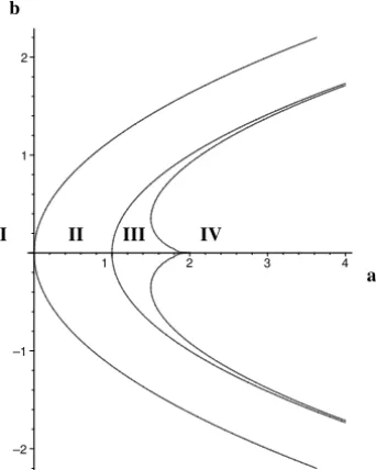
Schaeffer and Shearer classified quadratic models with isolated umbilic points by dividing the(a,b)-plane into four regions. This classification of models into Cases I-IV is based on the structure of rarefaction curves through the origin. The division of the parameter plane is illustrated in Figure 1. In detail, the curves separating the regions are as follows:
• Case I/II boundary: 4a−3b2 =0.
• Case II/III boundary: a−b2
−1=0.
• Case III/IV boundary:−32b4
+27+36(a−2)−4(a−2)2b2
+4(a−
–2 –1 1 2
1 2 3 4
a b
IV III
II I
Figure 1 – The Schaeffer-Shearer(a,b)-plane and case boundaries.
3.2 Fundamental wave manifold for homogeneous quadratic models
Many of the computations presented in this paper are based on the construc-tion of the fundamental wave manifoldW, which was introduced for quadratic models by Marchesin and Palmeira [17] and extended to general systems of con-servation laws in Ref. [8]. Points ofW represent shock wave solutions of the conservation laws. To each point inW is associated a dynamical system,viz., Eq. (2.9); whether or not a connection exists determines whether or not the shock is admissible.
The wave manifoldW is constructed by considering solutions(U−,U+,s)of the Rankine-Hugoniot condition (2.2). Although the solution set has a singularity at each point whereU− =U+, this singularity can be removed by introducing a new set of variables(U,R, ϕ,s). HereU =(u, v)T is the midpoint12(U−+U+)
is mapped to(U−,U+,s)through the relationships
U±=U± 1
2R cosϕ
sinϕ !
. (3.4)
This map remains smooth if each point (U,R, π/2,s) is glued to the point
(U,−R,−π/2,s), so we regard its domain asR2
×M2×R, whereM2is the Möbius strip parameterized by R andϕ. Expressed in terms of (U,R, ϕ,s), the Rankine-Hugoniot condition contains an explicit factor R, corresponding to trivial solutionsU+ = U−, which we eliminate. The remaining equation definesW.
For homogeneous quadratic models, the Rankine-Hugoniot condition is equiv-alent to
R −s I +F′(U) cosϕ
sinϕ !
=0, (3.5)
withF′being linear. Solutions satisfy either R=0 or
α(ϕ)u+β(ϕ)v=0, (3.6)
˜
α(ϕ)u+ ˜β(ϕ)v=s, (3.7)
whereα,β,α˜, andβ˜are homogeneous quadratic polynomials in cosϕand sinϕ
defined by
α(ϕ)u+β(ϕ)v=(−sinϕ,cosϕ)F′(U) cosϕ
sinϕ !
, (3.8)
˜
α(ϕ)u+ ˜β(ϕ)v=( cosϕ,sinϕ)F′(U) cosϕ
sinϕ !
. (3.9)
The wave manifold W comprises points (u, v,R, ϕ,s) satisfying Eqs. (3.6) and (3.7).
For the normal form (3.2), we have
α(ϕ)=bcos2ϕ+(1−a)cosϕsinϕ−bsin2ϕ, (3.10)
β(ϕ)=cos2ϕ−bcosϕsinϕ−sin2ϕ, (3.11) ˜
α(ϕ)=acos2ϕ+2bcosϕsinϕ+sin2ϕ, (3.12) ˜
The vector(α(ϕ), β(ϕ))never vanishes, by virtue of condition (3.3); indeed, the resultant ofαandβis−(a−b2
−1)2. Therefore Eqs. (3.6) and (3.7) are solved by
u = −β(ϕ)κ, (3.14)
v = α(ϕ)κ, (3.15)
s = De(ϕ)κ, (3.16)
whereκ ∈Rand
e
D(ϕ)=α(ϕ)β(ϕ)˜ −β(ϕ)α(ϕ).˜ (3.17)
For the normal form (3.2),
e
D(ϕ)=(b2−a)cos2ϕ+bcosϕsinϕ+sin2ϕ. (3.18) In summary, for a homogeneous quadratic model with an isolated umbilic point, points in the wave manifold can be parameterized by the variables
(R, κ, ϕ) ∈ R×R×(−π/2, π/2], with each point (R, κ, π/2) glued to the point(−R, κ,−π/2). The shock wave corresponding to(R, κ, ϕ)is obtained in the following way:
u± = −β(ϕ)κ±12Rcosϕ, (3.19)
v± = α(ϕ)κ±12Rsinϕ, (3.20)
s = De(ϕ)κ. (3.21)
Equations (3.19) and (3.20) define two projections fromW to state space: the
U−-projectionπ−:(R, κ, ϕ)7→ (u−, v−)and theU+-projectionπ+:(R, κ, ϕ)
7→(u+, v+).
We now define some additional expressions that will be used later:
D(ϕ)=α(ϕ)β′(ϕ)−β(ϕ)α′(ϕ), (3.22)
μ(ϕ)=(−sinϕ,cosϕ)F′′(0)∙ cosϕ
sinϕ !2
, (3.23)
˜
μ(ϕ)=(cosϕ,sinϕ)F′′(0)∙ cosϕ
sinϕ !2
, (3.24)
For the normal form (3.2),D(ϕ)≡a−b2
−1 is a nonzero constant,
μ(ϕ)=bcos3ϕ+(2−a)cos2ϕsinϕ−2bcosϕsin2ϕ−sin3ϕ, (3.26) ˜
μ(ϕ)=(acos2ϕ+3bcosϕsinϕ+3 sin2ϕ)cosϕ, (3.27) andB(ϕ)is simply(a−b2−1)μ(ϕ)˜ .
Remark. Even for general quadratic models,DandDeare homogeneous cubic polynomials, andBis a homogeneous quadratic polynomial, in cosϕand sinϕ.
3.3 Subsets of the fundamental wave manifold
3.3.1 Characteristic manifold
The characteristic manifold, denoted by C, is the R = 0 slice of the wave manifold. For a point inC,U−=U+=Uandsis an eigenvalue ofF′(U)(see
Eq. (3.5) with the factorRremoved). If a stateUis such that the eigenvalues of
F′(U)are real and distinct, then there are two different points inCthat project toU. In this case,Cis a two-fold covering of a sufficiently small neighborhood ofU.
3.3.2 Sonic loci
Theright sonic locus,SR, is the closure inWof the set of nontrivial shock waves such thatλi(U+)=s,i=1 or 2; theleft sonic locus,SL, is defined analogously by the conditionλi(U−)= s,i =1 or 2. For homogeneous quadratic models,
the right sonic locus (respectively, left sonic locus) consists of points(R, κ, ϕ)
that satisfy
∓1
2De(ϕ)R+B(ϕ)κ =0. (3.28) (See Ref. [24, pp. 316–317] for the proof.) The left sonic locus is the reflection, through the (κ, ϕ)-plane, of the right sonic locus, which is characterized as follows.
Lemma 3.1. If4a 6= 3b2, S
R is a ruled surface, in that its intersection with
each planeϕ = const.is a line. If4a = 3b2, SR is the union of such a ruled surface with the planeϕ= −tan−1(b/2). The same is true ofS
Proof. The resultant ofDeandμ˜ = B/(a−b2
−1)is(4a−3b2)2. Therefore, if 4a 6= 3b2, the vector (1
2De(ϕ),B(ϕ))never vanishes. Thus, for each ϕ, the solution set of Eq. (3.28) (with the upper sign) is a line. If, on the other hand, 4a=3b2, thenDe(ϕ)= [(b/2)cosϕ+sinϕ]2andμ(ϕ)˜ =3De(ϕ)cosϕ, so that the solution set is the union of the planeDe(ϕ)=0 with the ruled surface
−1
2R+ [3(a−b 2
−1)cosϕ]κ =0. (3.29)
3.3.3 Inflection locus
A point in theinflection locuslies in the characteristic manifold C and corre-sponds to a point in state space at which genuine nonlinearity fails. In general [8], the inflection locus is the common intersection of the sonic lociSL andSRwith C. From Eq. (3.28) we see that points in the inflection locus have R = 0 and eitherκ =0 orB(ϕ)=0. Thus the inflection locus comprises theϕ-axis (R =0 andκ =0) and the lines with R=0 andϕ =ϕi; hereϕi is aninflection angle,
i.e., a root ofB(ϕ)=0. The formula (3.27) forμ˜ =B/(a−b2−1)shows that the number of inflection angles is three if 4a <3b2, two if 4a
=3b2, and one if 4a>3b2.
3.3.4 Double sonic locus
Thedouble sonic locusis the closure of the set of nontrivial shock waves that lie on bothSL andSR. According to Eqs. (3.28) and Lemma 3.1: if 4a 6=3b2, the double sonic locus comprises the lines withκ =0 andϕ = ϕd, whereϕd is a
double sonic angle,i.e., a root ofDe(ϕ); and if 4a =3b2, the double sonic locus is the planeϕ = −tan−1(b/2). The formula (3.18) for De(ϕ)shows that there are no double sonic angles if 4a<3b2and there are two if 4a >3b2.
3.4 Proof of Proposition 2.1.
The following proof is an application of the formalism just developed.
the viscosity matrix Q is strictly stable for system (1.1) at a state U∗ if and only if the quantities tr[−s I +F′(U
∗)]and tr
Q−1
[−s I +F′(U
∗)] have the
same (nonzero) sign for each eigenvalues of F′(U
∗). Moreover, Theorem 5.8
of this reference implies that ifU∗andsare associated with a point(κ, ϕ)on the
characteristic manifoldCfor a homogeneous quadratic model, then
trQ−1−s I +F′(U∗) =κ
−1
2Q(ϕ)21D
′(ϕ)+Q(ϕ)
22D(ϕ)
; (3.30)
hereQ(ϕ)21andQ(ϕ)22are the(2,1)- and(2,2)-components, respectively, of the matrix
Q(ϕ)=O(ϕ)−1Q−1O(ϕ), (3.31) where
O(ϕ)= cosϕ −sinϕ
sinϕ cosϕ !
. (3.32)
Consequently the criterion for strict stability ofQatU∗ is that, for each corre-sponding point (κ, ϕ) on C, κD(ϕ) and κ−21Q(ϕ)21D′(ϕ)+Q(ϕ)22D(ϕ)
have the same nonzero sign. For a quadratic model written in the normal form (3.2),Dis a nonzero constant. Therefore the viscosity matrixQis strictly stable atU∗if and only ifκ 6= 0 andQ(ϕ)22 >0 for each corresponding point
(κ, ϕ)onC. Thus the viscosity matrixQis strictly stable at all statesU∗6=0 if and only if
(−sinϕ,cosϕ)Q−1 −sinϕ
cosϕ !
>0 (3.33)
for allϕ, or equivalently that the symmetric part ofQis strictly positive definite. Because a quadratic model in the normal form (3.2) has a symmetric Jacobian matrix F′, the equivalence of statements (2) and (3) is well known (see, e.g.,
Ref. [23, p. 398]). Indeed, a functionηis an entropy if and only ifF′is symmetric with respect to the quadratic formη′′, andηis compatible with Q if and only if the symmetric part of Qis strictly positive definite with respect toη′′; but if
η(U)= 12|U|
4 Transitional regions
In this section, we describe the subset ofW corresponding to transitional shock waves. This subset depends sensitively on the viscosity matrix Q. We con-sider quadratic models in Schaeffer-Shearer normal form (3.2) equipped with symmetric, strictly positive definite viscosity matrices. Admissibility of shock waves is not affected whenQis multiplied by a positive scale factor, so we are free to write
Q−1= 1 j j k !
, (4.1)
wherek >0 andk > j2.
4.1 Transitional waves
In general, it is difficult to characterize the set of transitional shock waves. How-ever, the following result greatly simplifies this characterization for homogeneous quadratic models with isolated umbilic points. The proof of this result, which is based on a theorem of Chicone [2], is due to Freistühler and Zumbrun [4].
Theorem 4.1. Suppose that system (1.1) is written in the normal form of Schaeffer-Shearer and equipped with a constant, symmetric, positive definite viscosity matrix Q. Then the orbit for any transitional wave is a straight line segment.
Proof. Multiplying the dynamical system (2.9) by Q−1/2 and substituting
b
U =Q−1/2bV, we obtain the system
b
V′(ξ )= −s Q−1Vb(ξ )+Q−1/2F(Q−1/2bV(ξ ))−Q−1/2[−sU−+F(U−)]. (4.2) According to Ref. [18], there exists a homogeneous cubic polynomialC ofU
such thatF =(C′)T. Let
D(V)=C(Q−1/2V)−1
2sV
TQ−1V
−VTQ−1/2[−sU−+F(U−)]. (4.3) Then
b
Thus the dynamical system (2.9) is linearly equivalent to a quadratic gradient system. For such a system, a saddle-saddle connection lies along a straight
line [2].
4.2 Straight-line connections
From Ref. [9], we have the following result concerning straight-line connections (for any type of shock wave).
Proposition 4.2. Let F be quadratic, and suppose that s, U−, and U+ 6=U− satisfy the Rankine-Hugoniot condition. Then the straight line segment between U− and U+is a connecting orbit if and only if there is a constantσ 6= 0such that1U =U+−U−satisfies
σQ1U = 1
2F
′′(0)
∙(1U)2. (4.5)
The orbit is traversed from U−to U+if and only ifσ <0.
In terms of coordinates forW,1U =R(cosϕ,sinϕ)T, so that Eq. (4.5) holds for someσ if and only if
0=(−sinϕ,cosϕ)Q−1F′′(0)∙ cosϕ sinϕ
!2
. (4.6)
The right-hand side of Eq. (4.6) resemblesμ(ϕ), defined by Eq. (3.23), except thatF′′(0)is replaced withQ−1F′′(0). We therefore denote the right-hand side
of Eq. (4.6) byμQ(ϕ). A rootϕv ofμQ(ϕ)is called aviscosity angle. Thus if two statesU−andU+are connected by a straight-line connection, then that orbit lies at a viscosity angle in state space. The expressionμQ(ϕ)is a homogeneous cubic polynomial in cosϕand sinϕ; in the generic case that the discriminant of
μQis nonzero, the number of viscosity angles is either one or three.
Proposition 4.2 also states that the straight-line connection is oriented from
U−toU+whenσ < 0. Again because1U = R(cosϕ,sinϕ)T, whereϕ =ϕv is a viscosity angle,
σ = 1
2R(cosϕ,sinϕ)Q
−1F′′(0)∙ cosϕ
sinϕ !2
which we write as
σ = 1
2Rμ˜Q(ϕ). (4.8) Thus the orbit orientation conditionσ <0 can be written
sgnR= −sgnμ˜Q(ϕv). (4.9)
If μ˜Q(ϕv) = 0, the viscosity angle ϕv is said to be exceptional [9]. At an exceptional viscosity angle, no straight-line connections are possible, since σ
=0. Exceptional viscosity angles occur when a viscosity angle coincides with a root ofμ˜Q(ϕ). This situation is avoided in the generic case that the resultant ofμQ andμ˜Qis nonzero.
4.3 Geometry of transitional surfaces
We define thetransitional surfaceto comprise points in the wave manifold corre-sponding to transitional shock waves,i.e., shock waves with viscous profiles that connect saddle points. For the quadratic models and viscosity matrices we con-sider, any transitional shock wave has a straight-line connection (Theorem 4.1). To determine the transitional surface, we seek straight-line connections joining saddle points.
In the previous subsection, we saw that a point inW corresponds to a shock wave with a straight-line connection if and only ifϕ=ϕvis a viscosity angle. A cross-sectionϕ =ϕvof the wave manifold is called aviscosity plane; there are from one to three viscosity planes. Thus the transitional surface is contained in the union of the viscosity planes and may consist of several disjoint connected components. However, not every viscosity plane contains a component of the transitional surface. We say that a viscosity angle isactiveif the corresponding viscosity plane contains a component of the transitional surface.
Consider the shock types of points of W. The signs of λ1(U−) −s and λ2(U−)−sare nonzero except at the characteristic manifoldCand the left sonic
locusSL, and the signs ofλ1(U+)−s andλ2(U+)−s are nonzero except atC
Lemma 4.3. Each connected component of the transitional surface is a con-nected component of a viscosity plane with the sonic loci and the characteristic manifold removed.
According to Lemma 3.1, either SL and SR contain the viscosity plane (if 4a =3b2andϕ
v = −tan−1(b/2)) or they intersect the viscosity plane in two lines through the origin that are reflections of each other through the lineR =0. In the former case, no transitional waves lie in the viscosity plane. Otherwise, after removingC, SL, and SR from the viscosity plane, several open sectors remain. In the following lemma, we determine which of these open sectors can be a component of the transitional surface.
Lemma 4.4. Any component of the transitional surface contained in the vis-cosity planeϕ =ϕvintersects the lineL(ϕv)along whichκ =0andϕ=ϕv.
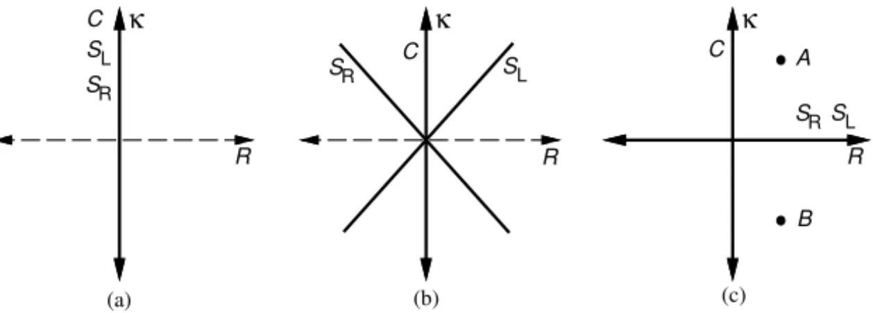
Proof. Depending of the configuration ofSL,SR, andCin the viscosity plane, two, four, or six open sectors remain. These possibilities are illustrated in Figure 2.
κ
R
κ
R κ
R S
R L
S
(a) (b) (c)
L
S S
R
S
RSL
C C
C
A
B
Figure 2 – Possible configurations ofSL,SR, andCin a viscosity plane.
Case (a): C,SL, andSRintersect the viscosity plane in a single line (i.e.,ϕv is an inflection angle). The two remaining open half planes both intersect the line L(ϕv).
Case (b): C, SL, and SR intersect the viscosity plane in three distinct lines. Consider a point with R 6= 0 lying onL(ϕv). Sinceκ = 0, the velocitys =
e
U+projections of this point are
U−= −
1
2Rcosϕv −12Rsinϕv
!
and U+=
1
2Rcosϕv 1
2Rsinϕv
!
. (4.10)
ThusU+= −U−, which implies thatF′(U+)= −F′(U−),λ1(U+)= −λ2(U−),
andλ2(U+)= −λ1(U−). With these restrictions on the shock and characteristic
velocities, this point can correspond to one of only three possible shock wave types: transitional(−,+,−,+), overcompressive(+,+,−,−), or totally ex-pansive(−,−,+,+).
If neither of the open sectors intersecting the lineL(ϕv)contains transitional shock waves, then one of the other open sectors must. Thus a sector containing transitional waves is separated from a sector containing either overcompressive or totally expansive waves by a single sonic surface. This, however, is impossible since, in crossing a single sonic surface, only one of the four quantitiesλ1(U−)−s, λ2(U−)−s,λ1(U+)−s, orλ2(U+)−s changes sign.
Case (c):C,SL, andSRintersect the viscosity plane in two distinct lines. In this case, the sonic loci both intersect the viscosity plane in the lineκ=0,i.e.,ϕvis a double sonic angle (De(ϕv)=0). Also,B(ϕv)6=0, since otherwise the entire viscosity plane is sonic according to Eq. (3.28). Thus there is no open sector containing the lineL(ϕv). We show that no transitional shock waves occur in this viscosity plane.
Consider two points AandBin the open quadrants of the viscosity plane that are reflections acrossκ = 0. According to Eqs. (3.19) and (3.20), theU− and
U+projections of AandB satisfy
U−A= −U+B, (4.11)
U+A= −U−B. (4.12)
BecauseDe(ϕv) = 0, the velocity of a shock wave corresponding to any point in this viscosity plane is zero. From Eqs. (4.11) and (4.12), we also deduce that λ1(U−A) = −λ2(U+B), λ1(U+A) = −λ2(U−B), λ2(U−A) = −λ1(U+B), and
must also correspond to a transitional shock wave. However, this is impossible because AandB are separated only by the left and right sonic loci. Therefore there are no transitional shock waves and the viscosity plane does not contain a component of the transitional surface in case (c). Lemma 4.4 does not specify which of the two open sectors containingL(ϕv)is a component of the transitional surface. Recall from Eq. (4.8) that the sign ofσ, which determines the orientation of the connecting orbit, depends on the sign of
R. The open sector that gives rise to correctly oriented orbits is thetransitional sector, determined by condition (4.9). In Section 5.2, we determine sgnμ˜Q(ϕv) precisely.
In the following theorem, we present the conditions that a viscosity angle must satisfy in order to be active.
Theorem 4.5. A viscosity angleϕvis active if and only if the following condi-tions are satisfied:
(1) μ˜Q(ϕv)6=0,i.e.,ϕvis not exceptional; and
(2) De(ϕv) >0.
Moreover, the corresponding transitional sector is the one containing the line L(ϕv)along whichκ =0andϕ =ϕvand havingsgnR= −sgnμ˜Q(ϕv).
Proof. Suppose thatϕv is active; we examine the viscosity plane associated with this angle. Condition (1) holds, as otherwise no straight-line connection occurs atϕvby virtue of Prop. 4.2 and Eq. (4.8). Condition (2) is established as follows.
From Lemma 4.4, we know that only an open sector containing the lineL(ϕv) can possibly be a component of the transitional surface. Consider the projections
U+andU−= −U+of a point on this line withR 6=0. As its shock speed is zero, this point corresponds to a transitional shock wave if and only if the eigenvalues of F′(U−) have opposite signs and the eigenvalues of F′(U−) have opposite signs. AsF′(U
−)= −F′(U+), this condition amounts to det(F′(U+)) <0. We
show that this inequality is equivalent to
e
BecauseF is a homogeneous quadratic polynomial, we have thatF′(U+) = F′′(0)U
+. AsR 6=0, the condition det(F′(U+)) < 0 is equivalent to
det
"
F′′(0) cosϕv
sinϕv
!#
<0. (4.14)
Inserting a rotation matrix does not affect the determinant; therefore the inequal-ity (4.14) is satisfied if and only if the following inequalinequal-ity holds:
det
"
cosϕv sinϕv −sinϕv cosϕv
!
F′′(0) cosϕv
sinϕv
!#
<0. (4.15)
The entries of the matrix appearing in this inequality may be identified by dif-ferentiating expressions (3.8)-(3.9) with respect to U. Thus we can rewrite inequality (4.15) as
det α(ϕ˜ v) β(ϕ˜ v)
α(ϕv) β(ϕv)
!
<0, (4.16)
which reduces to
˜
α(ϕv)β(ϕv)−α(ϕv)β(ϕ˜ v) <0. (4.17)
The left-hand side is−De(ϕv), so that det(F′(U+)) <0 if and only if condition (2)
holds.
Conversely, if conditions (1) and (2) hold, then a point with R6=0 on the line L(ϕv)provides an example of a transitional shock wave, so that the viscosity angleϕvis active.
Whenϕvis active, Lemma 4.4 and Eq. (4.9) determine the transitional sector.
4.4 Projection to state space
As restricted to a viscosity planeϕ =ϕv, the projectionsπ+andπ−defined
by Eqs. (3.19) and (3.20) can be written as
u+ v+ !
= −β(ϕv) 1
2cos(ϕv)
α(ϕv) 12sin(ϕv)
! κ R ! (4.18) and u− v− !
= −β(ϕv) − 1
2cos(ϕv)
α(ϕv) −12sin(ϕv)
! κ R
!
, (4.19)
respectively. Suppose that the matrices P+ and P− appearing, respectively, in
Eqs. (4.18) and (4.19) are nonsingular; this is true if and only ifα(ϕv)cos(ϕv)+
β(ϕv)sin(ϕv)6=0,i.e.,
μ(ϕv)6=0. (4.20)
Then the mapU− 7→ U+ = P+(P−)−1U
−, defined for statesU−in the
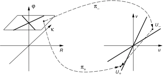
transi-tional wedge corresponding to viscosity angleϕv, is called thetransitional map forϕv. (See Fig. 3.) A stateU− in the transitional wedge and its image U+
under the transitional map are the end states of a transitional shock wave with a straight-line orbit. U − U+ R κ v u
ϕ π−
+ π
Figure 3 – The transitional map for a viscosity angleϕvwithμ(ϕv)6=0.
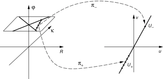
transitional planeϕ = ϕv, which is mapped via P+to a line segment of states U+, as in Figure 4. (By Eq. (3.11), the kernels of P+ and P− never coincide whenμ(ϕv)=0.) There is a transitional shock wave fromU−to each stateU+
lying on this line segment.
R
κ
v
u
ϕ
U
−
U
+ π+
π−
Figure 4 – The transitional map for a viscosity angleϕvwithμ(ϕv)=0.
Remark. An angleϕ satisfyingμ(ϕ) =0 is called abifurcation angle; such angles determine the secondary bifurcation loci in the wave manifold.
5 Classification of models
In this section, we determine the boundaries in the parameter plane that separate models with differing numbers of transitional regions. Many of the calculations presented in this section were carried out with the aid of the Maplesoftware package [1].
5.1 Classification according to the active region criterion
Motivated by Theorem 4.5, we now determine the parameter values such that the conditionDe(ϕv) >0 is satisfied. Recall that a viscosity angleϕvis a root of
μQ(ϕ). Usually, eachϕvcan be regarded as a function of the parameters of the model and the viscosity matrix. For eachϕv, there are curves in the parameter plane which separate those models for whichDe(ϕv) > 0 from those for which
e
where De(ϕ) and μQ(ϕ) have coincident roots. In order to determine these curves, we consider the resultant of De(ϕ) andμQ(ϕ), which vanishes if and only if the two polynomials have at least one coincident root. Direct calculation usingMapleshows that
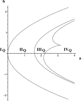
resultant(μQ,De)=(b2+bj+k−a)2(4a−3b2). (5.1) Each of the two factors of resultant(μQ,De)can vanish, and in Figure 5 we have drawn the zero-sets of these two factors in the(a,b)-plane for a particular viscosity matrix. In this figure, we have also drawn the curve representing the zero-set of the discriminant of μQ, which we compute below; upon crossing this curve from left to right, the number of roots ofμQ changes from three to one. The relative placement of the three curves remains the same as we vary the viscosity matrix because the three curves do not intersect, as we verify in the following two lemmas.
–2 –1 1 2
1 2 3 4
a b
IV III
II
IQ Q Q Q
Figure 5 – The case boundaries for a representative matrixQ(k=1.6 and j = −0.2). The left-most curve is defined by 4a −3b2 = 0; the middle curve is defined by a−(b2+bj+k)=0; and the right-most curve is defined by discriminant(μQ)=0.
Proof. Substitutinga=3b2/4 into the expressionb2
+bj +k−ayields
1 4b
2
+bj+k = 1
2b+ j
2
+k− j2, (5.2) which is positive ifk− j2>0. Hence, the two curves do not intersect.
Lemma 5.2. The curves a−(b2+bj+k)=0anddiscriminant(μQ)=0do
not intersect.
Proof. UsingMaple, we find that the discriminant ofμQ to be 61b2k2+4a2b2−52ab2k+32k3−4a3+32b4k−48ak2+24a2k
−44a2j2+b2j4+8b3j3+4k2j2+4b4j2+4a j4+40abj3 +32ak j2−20a2bj+64ab2j2+82b2k j2+100bk2j
+100b3k j+8bk j3+24ab3j−64abj k.
(5.3)
After substitutinga=b2
+bj+k, expression (5.3) simplifies to
4(k− j2)2 1
4b 2
+bj+k
, (5.4)
which is positive ifk− j2>0. Hence, the two curves do not intersect. In fact, the proofs above establish that the curves 4a−3b2
= 0, a−(b2 + bj +k) = 0, and discriminant(μQ) = 0 are ordered from left to right, in the sense that, for eachb, theacoordinates of points on the curves are so ordered. Therefore we can make the following definition.
Definition 5.3. We denote the region where a<3b2/4by I
Q; the region where 3b2/4 < a < b2 +bj +k by IIQ; the region where b2+bj +k < a and discriminant(μQ) > 0 by IIIQ; and the region wherediscriminant(μQ) < 0
by IVQ.
Remark. The IQ/IIQ boundary is exactly the Schaeffer-Shearer Case I/II boundary; and when Q = I, the IIQ/IIIQ and IIIQ/IVQ boundaries reduce to the Case II/III and Case III/IV boundaries, respectively.
Theorem 5.4. In region IQ, there are three active viscosity angles; in region
IIQ, there are two active viscosity angles; and in regions IIIQ and IVQ, there are
no active viscosity angles.
Proof. Within each region, the number of roots of μQ(ϕ) and the ordering of the roots ofDe(ϕ) andμQ(ϕ) along (−π/2, π/2] are the same. To prove the theorem, we choose a simple representative model within each region and examine the roots of the two polynomials for this model.
We letb=0 and Q = I,i.e.,k =1 and j =0. For these parameter values, we havea <0 in region IQ, 0<a<1 in region IIQ, 1<a<2 in region IIIQ, anda >2 in region IVQ. The roots ofμQ(ϕ)are
ϕv1=arctan(−√2−a), ϕv2=0, and ϕv3=arctan(√2−a), (5.5) and the values ofDe(ϕ)at these angles are
e
D(ϕv1)=
2(1−a)
3−a , (5.6)
e
D(ϕv2)= −a, (5.7)
e
D(ϕv3)= 2(1−a)
3−a . (5.8)
In region IQ, we have De(ϕ) > 0 for ϕ = ϕv1, ϕv2, andϕv3; hence, all three viscosity angles are active. In region IIQ, we haveDe(ϕ) >0 for ϕ =ϕ1
v and
ϕ=ϕv3only; hence, only two of the viscosity angles are active. In region IIIQ, we haveDe(ϕ) <0 forϕ =ϕ1
v,ϕv2, andϕ =ϕv3; hence, there are no active viscosity angles. Finally, in region IVQ, we haveDe(ϕ) <0 for the only viscosity angle
ϕ=ϕv2; hence, there are no active viscosity angles. In the region in the parameter plane corresponding to three real viscosity angles, we can order the angles asϕ1
v < ϕv2< ϕv3within(−π/2, π/2]. Upon crossing the 4a−3b2boundary, it isϕv2that no longer satisfies condition (4.13).
5.2 Classification according to the orientation criterion
condition sgnR = −sgnμ˜Q(ϕv)corresponds to properly oriented transitional shock waves. To use this condition, we must determine the sign ofμ˜Q evaluated at a viscosity angleϕv. UsingMaple, we have the following expression:
resultant(μQ,μ˜Q)=(4a−3b2)(k− j2)2
× (a2j2+2a j2+b2j2+ j2+6bj+2abj+2abj k+6bj k − 4ak+4k2+4k+1+a2−2a+4b2k+4b2+b2k2)
(5.9)
Because the viscosity angles are exactly the roots of μQ, the zero-set of the resultant ofμQandμ˜Qcomprises curves on whichμ˜Q(ϕv)=0 for some viscos-ity angleϕv,i.e., some viscosity angle is exceptional. The first factor vanishes at the Schaeffer-Shearer Case I/II boundary, which is the IQ/IIQboundary. The second factor never vanishes since Q is positive definite, and the third factor plays no role, according to the following lemma.
Lemma 5.5. The expression
a2j2+2a j2+b2j2+ j2+6bj+2abj+2abj k+6bj k
−4ak+4k2+4k+1+a2−2a+4b2k+4b2+b2k2 (5.10) vanishes only in the region in the parameter plane where there are no active viscosity angles.
Proof. Expression (5.10) is a quadratic polynomial ina, the discriminant of which is
−4(2j+2b+bj2+2k j+bk)2. (5.11) Therefore expression (5.10) has imaginary roots (and hence never vanishes) except when the discriminant (5.11) is zero. The discriminant vanishes when
b = −2j(1+k)
2+k+ j2. (5.12) For this value ofb, expression (5.10) vanishes when
a = 2k
2
+5k+2− j2
We are concerned only with active viscosity angles; therefore we shall determine whether this value ofasatisfiesa<b2
+bj+kwhen Eq. (5.12) holds. After some algebraic manipulations, we see that a < b2
+bj +k if and only if
k3+5k2+8k−2k j2−2k2j2+k j4+ j4+4<0. (5.14) However, the left-hand side can be rewritten as
(k− j2)2(1+k)+4(1+k)2, (5.15) which is manifestly positive. Therefore any value of a that would make the factor (5.10) vanish lies in the region where there are no viscosity angles.
From this lemma, we see thatμ˜Q(ϕv)changes sign only across the Case I/II boundary. At this boundary, we haveϕv2coinciding with a root ofμ˜Q(ϕ). (See the discussion after Theorem 5.4.) Fora > 3b2/4, ϕ2
v does not correspond to a transitional region, so we do not consider it; however, whena < 3b2/4, we do need to considerϕ2
v. As in the proof of Theorem 5.4, we choose the simple representative model, b = 0 and Q = I, and examine the sign of μ˜Q(ϕ) at each of the viscosity angles. Whena < 3b2/4, we have
˜
μQ(ϕv2) < 0, since a <0. The other two viscosity anglesϕv1andϕv3giveμ˜Q >0 for models with transitional shock waves.
Therefore for all models with transitional shock waves, we haveμ˜Q(ϕ) >0 forϕv1 andϕv3, and for models whereϕ2v is an active viscosity angle, we have
˜
μQ(ϕ2v) <0. This concludes the proof of the following theorem.
Theorem 5.6. For all models, in the viscosity planes corresponding toϕ1vand ϕ3
v, the transitional sector is the sector containing the ray on whichκ =0and R<0. For models havingϕv2as an active viscosity angle, in the viscosity plane corresponding toϕ2v, the transitional sector is the sector containing the ray on whichκ=0and R>0.
6 Conclusion
as the admissibility criterion. The viscosity matrices we used were symmetric and positive definite.
Our primary focus has been the behavior of transitional shock waves. For these models, we have precisely described the transitional surface — the subset of the wave manifold that corresponds to transitional shock waves. The transi-tional surface consists of components that lie in planes that correspond to active viscosity angles. We have derived a condition for determining exactly when a viscosity angle is active. With this condition, we have determined the boundaries (in terms of the model and viscosity matrix parameters) where the number of active viscosity angles changes.
The results we have concerning the effects of viscous terms on the solutions of Riemann problems are primarily analytical. However, they have immediate implications for numerical analysis. In finite-difference solvers for conservation laws, the use of artificial viscosity is common. From our work, we can see that different viscosity matrices will result in different solutions; hence, care must be chosen to ensure that the form of the viscosity accurately reflects the physics of the problem being modeled.
Acknowledgments. This work has been supported in part by: the Henry Luce Foundation through a Clare Boothe Luce Professorship; the NSF under Grant DMS-9732876; the DOE under Grant DE-FG02-90ER25084; MCT under Grant PCI 650009/97-5; FAPERJ under Grant E-26/150.936/99; CNPq under Grant 451055/00-4; and FINEP under Grant 77970315-00.
We thank Profs. H. Freistühler and K. Zumbrun for providing the proof of Theorem 4.1. We also thank Prof. D. Marchesin and the Instituto de Matemática Pura e Aplicada for generous support during the writing of the manuscript.
REFERENCES
[1] B. Char, K. Geddes, G. Gonnet, B. Leong, M. Monagan and S. Watt, Maple V Library Reference Manual. Springer-Verlag, New York–Heidelberg–Berlin, 1991.
[2] C. Chicone, Quadratic gradients on the plane are generically Morse-Smale. J. Differential Equations,33(1979), 159–166.
[4] H. Freistühler and K. Zumbrun, Private communication, 1996.
[5] I. Gelfand, Some problems in the theory of quasi-linear equations. Uspekhi Mat. Nauk,
14(1959), 87–158.
[6] J. Hurley,Effects of Viscous Terms on Solutions of Riemann Problems. PhD thesis, State Univ. of New York at Stony Brook, 1995.
[7] J. Hurley and B. Plohr, Some effects of viscous terms on Riemann problem solutions. Mat. Contemp.,8(1995), 203–224.
[8] E. Isaacson, D. Marchesin, C.F. Palmeira and B. Plohr, A global formalism for nonlinear waves in conservation laws.Comm. Math. Phys.,146(1992), 505–552.
[9] E. Isaacson, D. Marchesin and B. Plohr, Transitional waves for conservation laws. SIAM J. Math. Anal.,21(1990), 837–866.
[10] E. Isaacson, D. Marchesin, B. Plohr and J.B. Temple, The Riemann problem near a hyper-bolic singularity: the classification of quadratic Riemann problems I.SIAM J. Appl. Math.,
48(1988), 1009–1032.
[11] E. Isaacson and J.B. Temple, The Riemann problem near a hyperbolic singularity II.SIAM J. Appl. Math.,48(1988), 1287–1301.
[12] E. Isaacson and J.B. Temple, The Riemann problem near a hyperbolic singularity III.SIAM J. Appl. Math.,48(1988), 1302–1312.
[13] P. Lax, Hyperbolic systems of conservation laws II.Comm. Pure Appl. Math.,10(1957), 537–566.
[14] P. Lax, Shock waves and entropy. In E. Zarantonello, editor,Contributions to Nonlinear Functional Analysis, pages 603–634. Academic Press, New York, 1971.
[15] T.-P. Liu, The Riemann problem for general 2×2 conservation laws. Trans. Amer. Math. Soc.,199(1974), 89–112.
[16] A. Majda and R. Pego, Stable viscosity matrices for system of conservation laws.J. Differ-ential Equations,56(1985), 229–262.
[17] D. Marchesin and C.F. Palmeira, Topology of elementary waves for mixed systems of conservation laws.J. Dynamics Differential Equations,6(1994), 427–446.
[18] D. Schaeffer and M. Shearer, The classification of 2×2 systems of non-strictly hyperbolic conservation laws, with application to oil recovery. Comm. Pure Appl. Math.,40(1987), 141–178.
[19] D. Schaeffer and M. Shearer, Riemann problems for nonstrictly hyperbolic 2×2 systems of conservation laws.Trans. Amer. Math. Soc.,304(1987), 267–306.
[21] M. Shearer, The Riemann problem for 2×2 systems of hyperbolic conservation laws with Case I quadratic nonlinearities.J. Differential Equations,80(1989), 343–363.
[22] M. Shearer, D. Schaeffer, D. Marchesin and P. Paes-Leme, Solution of the Riemann problem for a prototype 2×2 system of non-strictly hyperbolic conservation laws. Arch. Rational Mech. Anal.,97(1987), 299–320.
[23] J. Smoller,Shock Waves and Reaction-Diffusion Equations. Springer-Verlag, New York, second edition, 1994.
[24] S. ˇCani´c and B. Plohr, Shock wave admissibility for quadratic conservation laws.J. Differ-ential Equations,118(1995), 293–335.