Braz. J. Chem. Eng. vol.19 número4

ISSN 0104-6632 Printed in Brazil

Vol. 19, No. 04, pp. 457 - 466, October - December 2002

of Chemical

Engineering

A GENERAL FRAMEWORK FOR SIMULTANEOUS

CYCLIC SCHEDULING AND OPERATIONAL

OPTIMIZATION OF MULTIPRODUCT

CONTINUOUS PLANTS

A.Alle and J.M.Pinto

Department of Chemical Engineering University of Sao Paulo, USP, Av. Prof. Luciano Gualberto Travessa 3, 380, 05508-900, Sao Paulo - SP, Brazil.

E-mail: [email protected]

(Received: March 5, 2002 ; Accepted: May 27, 2002)

Abstract - This paper addresses the problem of integrating in a single model operational optimization and

cyclic scheduling of continuous plants. Considered are multiproduct, multistage plants with finite intermediate storage capacity (FIS). A combined optimization approach introduces synergic effects for more effective scheduling and plant operation (Alle and Pinto, 2001a,b). The representation proposed for this problem results in an MINLP model with a nonconvex feasible region and nonconvex objective function. In order to deal with nonconvexity, a spatial branch-and-bound global optimization algorithm is applied. Results show that the global approach is effectively able to yield more profitable solutions than those obtained by local optimization methods.

Keywords: scheduling, optimization of process conditions, continuous plants, mathematical programming, global optimization.

INTRODUCTION

In multiproduct continuous plants, scheduling involves several trade-offs between length of production cycle, inventory levels, changeover times and costs (Pinto and Grossmann, 1994). The introduction of variable processing rates brings additional interactions into the scheduling model. The faster a unit runs, the lower its yield due to the shortening of residence times. Moreover, operational costs may increase. On the other hand, the unit would be free in a shorter period of time. Alle and Pinto (2001a,b) presented the TSPFLOP model, which incorporates variable processing rates and yields for simultaneous scheduling and operational optimization of these plants. Results showed that a combined optimization approach may better capture the complexity of the trade-offs

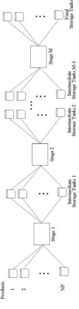
Given is a number of specified products (i=1…N) that are to be produced in a continuous plant consisting of several stages that are interconnected by intermediate inventory tanks for each product (Fig. 1). Each stage consists of one production line, which is interconnected with a fixed topology in order to perform a set of operations (reactions, separations etc.). Transition times that arise between the processing of two successive products are sequence dependent. Constant demand rates in the form of lower bounds that are to be satisfied are also given. Intermediate capacities are limited. Final capacity is not limiting and may be neglected. Moreover, stages may have their processing rates changed within a range. The processing yield in a stage may depend on its processing rate.

The following are the assumptions for modeling the problem (Alle and Pinto, 2001a):

A1)Every product must be processed in the same sequence at all stages (i.e., flowshop plant);

A2)Intermediate inventory depends on the maximum level of material accumulated, as in Buzacott and Ozkarahan (1983).

A3)Inventory cost of final products depends on the average amount of material to be stored, as in Sahinidis and Grossmann (1991).

A4)Stages must operate continuously within one cycle, i.e., waiting times are not allowed between operations once production has started.

A5) The product yield in every stage is an exponential decaying function of the processing rate, as in Alle and Pinto (2001a,b).

The problem then consists of determining the following items for a cyclic scheduling:

(a) sequence of products, (b) length of cycle time, (c) length of production times, (d) amounts to be produced, (e) levels of intermediate storage and (f) processing rates for every product in stages. The objective is the maximization of profitability (profit per unit of time), which includes income from the

more general case where every stage may have its rate adjusted.

Binary variables zij are used to determine product

sequence:

zij : 1 if product i precedes product j; otherwise 0.

As the plant is a flowshop, every product j must be preceded by the same product i at all stages. Only one product succeeds and precedes the other, as shown in (1).

1 , 1

ij ij

i i

z = ∀j z = ∀i

∑

∑

A transition time, τijm, and a transition cost, Ctrijm,

are incurred every time a unit changes from the production of product i to that of another product, j. The overall transition cost for a product i in a cycle Ct is given by (2).

i ij ijm

j m

Ct =

∑ ∑

The total amount of product i produced at stage m, Wim (ton), during one subcycle is the product of

the processing rate, γim (ton.h-1), and processing time, Tpim (h), as follows:

im im im

W = γ Tp ∀i, m (3) The amount produced at stage m must be completely consumed at stage m+1 in order to avoid accumulation of material within cycles.

im im 1 im 1

W = α ₊ W ₊ i, m 1...M 1∀ = − (4)

The mass balance coefficient, αim, is the inverse

of process yield of product i at stage m. It is assumed to depend on the processing rate.

(

)

im exp im/ bim i, m

Figure 1:

Multipr

oduct, c

y

clic conti

nuous pl

ants with interm

i i1 i1

The total demand for final products must be satisfied at the end of the cycle:

iM i

W ≥d Tc i∀ (8) The maximum level of intermediate inventory Imaxim (ton) is modeled as in Alle and Pinto (2001

a,b) with the aid of binary variables yim , defined as

follows:

yim : 1 if processing of product i finishes at stage m

before starting processing at stage m+1; otherwise, 0. The continuous variable Invim (ton) is defined as

the difference between Wim and the maximum

inventory level, Imaxim. Therefore,

im im im

Imax W Inv i, m 1...M 1

= −

∀ = − (9)

im

up

im im

0≤Inv ≤y W i, m 1...M 1∀ = − (10)

im

im im im im im 1

up im

0 Inv (Ts Tp Ts )

(1 y )W i, m 1...M 1

+

≤ − δ + − ≤

≤ − ∀ = −

(11)

where auxiliary variable δim is defined as follows:

im im i, m 1...M 1

δ ≤ γ ∀ = − (12)

im im 1 im 1+ + i, m 1...M 1

δ ≤ α γ ∀ = − (13)

As the plant has finite intermediate storage capacity (FIS), there is a limit on the storage capacity of the intermediate tanks:

im

up im

Imax ≤Imax i, m 1...M 1∀ = − (14)

As the plant is a flowshop, the processing of product i at stage m must start (end) before the start (end) of processing of the same product at stage m+1:

im im 1

im im im 1 im 1

Ts Ts and

Ts Tp Ts Tp i, m 1...M 1

+

+ +

≥

+ ≥ +

∀ = − ₍₁₆₎

As the schedule is cyclic, product 1 is arbitrarily chosen as the first to enter the production line:

11 i1 i11

i

Ts =

∑

(17) At any stage, the sum of the total occupation time plus the transition times for all products must not exceed the cycle time, Tc.

im ij ijm

i i j

Tc≥

∑

∑∑

(18) Every unit has a processing or operational cost for every product i, OCim, that is assumed to be

proportional to the processing rate, γim; the total

amount processed, αimWim; and a cost coefficient,

Coim:

im im im im im

OC =co γ α W i, m∀ ₍₁₉₎

M 1

i iM i i i im im im im im im

i m m

1

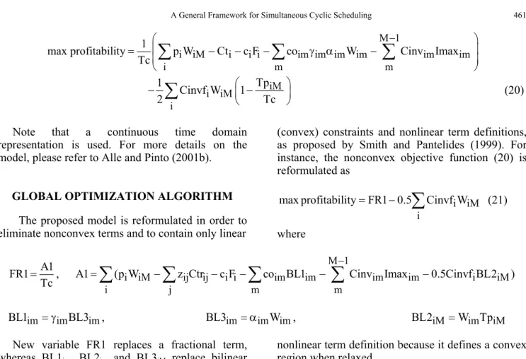
max profitability p W Ct c F co W Cinv Imax Tc

−

 

 

= − − − γ α −

 



∑

∑

∑

_{i iM} iM

i

Tp 1

Cinvf W 1

2 Tc

 

− _ − _

 

∑

Note that a continuous time domain representation is used. For more details on the model, please refer to Alle and Pinto (2001b).

GLOBAL OPTIMIZATION ALGORITHM

The proposed model is reformulated in order to eliminate nonconvex terms and to contain only linear

(convex) constraints and nonlinear term definitions, as proposed by Smith and Pantelides (1999). For instance, the nonconvex objective function (20) is reformulated as

i iM

i

max profitability=FR1 0.5−

∑

where A1 FR1 Tc = , M 1

i iM ij ij i i im im im im i iM

i j m m

A1 (p W z Ctr c F co BL1 Cinv Imax 0.5Cinvf BL2 )

−

=

∑

∑

∑

∑

BL1_im= γ_imBL3_im, BL3_im = α_imW_im, BL2_iM =W Tp_{im iM} New variable FR1 replaces a fractional term,

whereas BL1im, BL2im and BL3iM replace bilinear

terms; A1 replaces the sum that is the numerator of the fractional term. All constraints that contain nonlinear terms are submitted to similar transformation, except constraint (5). Actually, this equation may be relaxed to

(

)

im exp im/ bim i, m

α ≥ γ ∀

(22) without changing the global optimum. The reason is that inequality (22) must be active in the global optimum since the smaller the αim (i.e, the greater the yield) for a given γim, the greater the

plant profitability. Since the OA/ER/AP algorithm (Viswanathan and Grossmann, 1990) used here is based on equality relaxation, constraint (5) does not need to be replaced by a linear constraint and a

nonlinear term definition because it defines a convex region when relaxed.

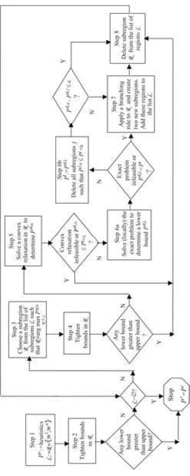
After the replacements, the global optimization algorithm shown in Fig. 2 is applied. It is a spatial branch-and-bound, based on Horst and Tuy algorithm (1993) general formulation, extended by Quesada and Grossmann (1995) and Ryoo and Sahinidis (1995, 1996), as described by Smith and Pantelides (1999). The algorithm makes use of the nonconvex MINLP reformulated model to generate lower bounds for the max problem and of a MINLP convex relaxation subproblem to find upper bounds. The convex relaxation is obtained through substitution of the nonlinear term definitions (fractional and bilinear terms) by new variables that are constrained by linear over- and under-estimators such as those from McCormick (1976), shown in Table 1.

Table 1: McCormick over- and underestimators for bilinear and fractional terms.

lo lo lo lo

im im im im im im im

BL ≥B L + B L −B L

Underestimators

{

im im im im im im im

BL ≥B L + B L −B L

lo up lo up

im im im im im im im

BL ≤B L + B L −B L

Bilinear term

im im im

BL ≡B L

Overestimators

{

im im im im im im im

BL ≤B L + B L −B L

lo lo lo lo

im im im im im im im

F ≥FR R +FR R −FR R

Underestimators

{

im im im im iM iM iM

F ≥FR R +FR R −FR R

lo up lo up

im im iM im im im im

F ≤FR R +FR R −FR R

Fractional term im im im F FR R ≡

Overestimators

{

Figure 2:

Flow diagram

for the global optim

ization algorithm

RESULTS

The spatial branch-and-bound algorithm was implemented in GAMS (Brooke et al., 1998). The MINLP solver used for both the nonconvex problem and the convex relaxation subproblem is DICOPT++ based on the OA/ER/AP method (Viswanathan and Grossmann, 1990). CONOPT2 (Drud, 1992) and XPRESS 12.5 solver (Dash Associates, 1999) were the solvers for the NLP subproblems and MILP master problems, respectively. The ε (global optimality gap) adopted is 1 %.

Table 2 shows the relative difference, ∆P*, between global and local optimal profitability for different problems. Global optimization yields solutions as good as or better than the straightforward local optimization procedure at the expense of a much larger computational effort, attributed mainly to steps 2 and 4 of the algorithm

(Smith and Pantelides, 1999).

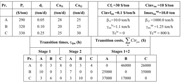
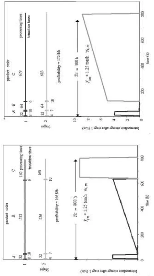
Table 3 contains data on a plant with two stages that processes three products. Fig. 3 shows the difference between global and local optimal schedules for this plant. The profitability increases 3.6% from the local to the global optimum. Upper bounds of Tc and processing rates are all active in both solutions. Note the large difference between the processing times for products B and C in each schedule as well as the different inventory control profiles.

Note, however, that global optimization performance highly depends on the quality of the convex relaxation. The closer the relaxed model to the exact one, the better the algorithm performs. As seen in Table 4, tight bounds for cycle time Tc are essential for a good relaxation. In fact, Tc bounds most of the variables in the model. As a consequence, the algorithm performance is very sensitive to Tc bounds.

Table 2: Results for local and global optimization.

Problem size Local opt. Global opt.

Products Stages ∆P

*

CPU(s) CPU (s) Iterations

3 2 3.6% 0.4 32.5 9

4 2 0% 1.7 25.9 1

5 3 0% 5.0 101.2 1

Table 3: Plant data for the example of the 3-product-2-stage plant.

Pr. Pi di Coi1 Coi2 Cfi =30 $/ton Cinvim =10 $/ton

($/ton) (ton/d) (ton/d) (ton/d) Cinvfim =0.1 $/ton/h Imaximup=10.0 ton

A 290 0.05 28 25 βi1=10.0 ton/h βi2 =1000.0 ton/h

B 320 0.10 20 25 γimlo=1.1 ton/h γimup =1.25 ton/h

C 330 0.25 25 30 Tclo _{= 0 Tc}up _{= 800 h}

Transition times, τijm (h) Transition costs, ijm

m

Ctr

∑

Stage 1 Stage 2 Stages 1+2

Pr. A B C A B C A B C

A 0 3 8 0 3 4 0 46000 26000

B 10 0 3 7 0 0 25000 0 35000

C 3 6 0 3 10 0 37000 17000 0

Table 4: Dependence of algorithm performance on Tc bounds (3 product/2 stage example).

Tcup Tclo Initial relaxation gap Iterations

800 0 4.8 % 9

1100 0 9.8% 11

Figure 3:

Local (left) and global (right)

optim

al schedules for a

continuous m

u

CONCLUSIONS

A general framework model for global optimization of the simultaneous problems of scheduling and operating conditions for continuous multiproduct plants was developed. The model extends Alle and Pinto’s (2001a,b) formulation to a more general case, where operating conditions (processing rates and yields) are allowed to vary at every plant stage. A spatial branch-and-bound algorithm was successfully applied to achieve globally optimal solutions. Results showed that the difference between a local and a global optimal schedule means a completely different way of planning production.

NOMENCLATURE Sets

Products i, j = 1,..., N Stages m = 1,..., M

Binary Variables

xim denotes whether the production of i in

stages m and m+1, occurs simultaneously

zij denotes whether product i is

immediately preceded by j

Continuous Variables

Iim intermediate inventory level of product i

in stage m

Invim difference between amount produced

and maximum inventory level of product i between stages m and m+1 Tc cycle time

Tpim processing time of product i in stage m

Tsim start time of product i in stage m

Wim amount of product i produced in stage

m

Fi amount of raw material consumed by

product i

Parameters

Cinvfi cost coefficient for inventory of final product i

Cinvim cost coefficient for inventory of product

i in stage m

Co operating cost coefficient for processing

product i at stage m

Ctrijm cost of transition between product i and

product j at unit m

di, pi minimum demand rate and price of

product i

Imaxim maximum inventory capacity for

product i after stage m

UIim UTim upper bounds of processing time and

inventory of product i in stage m

*

P

∆ *global *local * global Profitability Profitability 100% Profitability  ₋   _{ ×}    

τijm transition time from product i to product j in stage m

γim αim processing rate and mass balance

coefficient of product i in stage m

ACKNOWLEDGEMENT

The authors would like to acknowledge the support received from FAPESP (Fundação de Amparo a Pesquisa do Estado de São Paulo) under grants 99/02657-8 and 98/14384-3.

REFERENCES

Alle, A. and J.M. Pinto (2001a). Simultaneous Scheduling and Operational Optimization of Multiproduct Continuous Plants. Proceedings of the IFAC Symposium on Dynamics and Control of Process Systems 2001, DYCOPS 6, Korea, 212. Alle, A. and J.M. Pinto (2001b). Simultaneous

Scheduling and Operational Optimization of Multi-product Continuous Plants. Ind. Engng. & Chem. Res. /accepted for publication/.

Brooke, A., D. Kendrick and A. Meeraus (1998). GAMS - A Users’ Guide. The Scientific Press, Redwood City, CA.

Buzacott, J.A. and I.A. Ozkarahan (1983). One- and Two-Stage Scheduling of Two Products with Distributed Inserted Idle Time: the benefits of a Controllable Production Rate. Naval Res. Logist. Q., 30, 675.

Dash Associates (1999). XPRESS-MP Optimisation Subroutine Library. Reference Manual. Release 12, Blisworth House, Blisworth, UK.

Drud, A.S. (1992). CONOPT- A Large-Scale GRG Code. ORSA J. on Computing. 6, 207.

Plants. Comp. Chem. Engng., 18, 797.

Quesada, I. and I.E. Grossmann (1995). A Global Optimization Algorithm for Linear Fractional and Bilinear Programs. Journal of Global Optimization, 6, 39.

Ryoo, H.S. and N.V. Sahinidis (1995). Global

Algorithm for the Global Optimisation of Nonconvex MINLPs. Comput. Chem. Engng., 23, 459.