A Work Project, presented as part of the requirements for the Award of a Master’s
Degree in Finance from the NOVA – School of Business and Economics.
Systemic Risk for Financial Institutions in UK
Pavel Solomin #690
A Project carried out under the supervision of:
Prof. Paulo M. M. Rodrigues
2
Content
Abstract ... 3
1. Introduction ... 3
2. Literature Review ... 5
3. Econometric Approach ... 6
3.1. Volatility Modeling ... 9
3.2. Conditional Correlations ... 10
3.3. Tails Expectation ... 11
4. UK Financial Institutions ... 12
4.1. The Sample ... 12
4.2. Components of MES ... 14
4.3. Behavior of MES by Sub Sectors ... 15
4.4. Validity of MES estimates ... 15
4.5. Currency Effects ... 16
5. Conclusion ... 18
3
Abstract
Marginal Expected Shortfall (MES) is an approach used to measure the systemic risk
financial institutions face. It estimates how significantly systemic events (poor market performance, out of 1.6 times Standard Deviation borders) are expected to affect market
capitalization of a particular firm. The concept was developed in the late 2000s and is widely used for cross-country comparisons of financial firms. For the purposes of generalization of this technique it is often used with market data containing
non-domestic currencies for some financial firms. That may lead to results having currency noise in them as it is shown for 77 UK financial firms in our analysis between 2001 and
2014.
1.
Introduction
After the financial market crashes in the US and Europe in the late 2000s it became
evident that financial institutions are more fragile than what people thought. During the recession an alarming fact showed up again: a significant external shock affecting a
particular financial market (or, let’s say, a particular stock exchange) of a given country leads to surge in prices of stocks traded in that market which causes the loop of crisis. That happens when uncertainty increases in a stock exchange and investors move to less
risky assets than stocks and especially shares of financial institutions. In comparison with non-financial firms, financial firms have stricter requirements for the structure of
their liabilities. Because of that, in case of substantial loss (or assets’ revaluation due to market crash) they would be obliged to raise more capital to satisfy the requirements. That means that all the financial institutions meet a specific type of risk in financial
markets – their particular risk of loss in case of a market crash – actually, the main question is how much they expect to lose (how much shareholders are expected to raise
4
This rationale lead to the development of more sophisticated financial regulation tools
named “Macroprudential regulation” which includes the process of “developing a more
robust financial system” in its aims (Galati & Moessner, 2013).
A special class of econometric techniques exists for these purposes. The first is the
widely used VaR approach (Value at Risk – internal banks’ technique for asset management). However, some papers argue that Expected Shortfall (ES) is a better
measure for risk and, actually, more universal, and able to be implemented for more types of risk (Acerbi & Tasche, 2001). As an alternative there is another type of approach called the CoVaR, models which use an extended and generalized VaR
concept. Basically, it considers conditional VaR under the assumption of interconnections and spillovers (since it uses conditional expectations) among the
elements of a bank’s portfolio (Adrian & Brunnermeier, 2008); these models showed high predictable power. VaR and CoVaR models, however, being widely used, are out of the focus of this study; this study mainly focuses on ES and MES (marginal expected
shortfall).
Intuitively, systemic risk measures are likely to be dependent on the risk (especially the
consequences of “tail events”) that institutions bear. Higher risks taken often show themselves through relatively higher financial leverage and higher volatility of assets’ prices and market capitalization. But it should also be analyzed, whether the
institution’s portfolio value strongly depends on the market condition. If the answer is
“yes”, that would mean more fragility in crises – a very important factor (negative externality) which should be taken into account.
5
worldwide: the concept allows the risk measure to be aggregated over economies or
industries. But when there is a need to use non-domestic currency, some problems may arise: different currencies, even for the same data, may originate noisy MES estimates. This study is an attempt to investigate if such differences are significant and how (if
they exist) they may be interpreted.
2.
Literature Review
The MES estimator was introduced as an extended concept from banks’ internal procedures to measure the risk of their own portfolios (Acharya, et al., 2010). It measures the externalities that risk-taking financial institutions meet in case of a
systemic crisis. The authors also introduced a systemic risk-based mechanism of regulation (taxation) which makes financial institutions manage their assets taking into
account the systemic risk coming from financial markets. The tests performed have shown significant predictability of MES to SCAP1 Shortfall for the US banks over the largest US financial firms in 2007-2008.
Another study of the US financial sector using the MES approach (Brownless & Engle, 2010), however, with differently measured components of MES (using multivariate
GARCH and DCC methods together with nonparametric estimators for the tail expectation) captured the dynamics of MES for different sub-industries. As observed,
the main contributors to MES of a particular firm are firm’s leverage, size, volatility of
assets’ returns and its relation with the market. Moreover, leverage affects MES more when the overall market falls. It was also discovered that the new MES estimation
techniques have less bias in “extreme” samples in comparison with the “historical” MES used in previous studies.
1
6
The extension of this concept to European financial markets (Engle, et al., 2014)
proposed a rank of European financial institutions and argues that the European financial system takes more risk than US financial firms do. The model included the analysis of risks at the international, country-wide and firm level to capture all the
interconnections that arise between the international European financial market and a particular firm. Among the firms in the sample some firms were found as “too big to be
saved”: the expected amount of money needed to save them in case of another crisis reached a significant percentage of the domestic country’s GDP (4-5%).
Some papers discussed even wider applications, e.g. the application of these techniques
to analyze systemic risk of financial institutions in G-20 countries (Corvasce, 2013). The tests performed have shown that the MES estimates (also jointly with financial
leverage measures) were significant and robust predictors of market capitalization variation (during Jul 2007 - Dec 2008) over financial institutions in North American, European, and Asian economies.
3.
Econometric Approach
The approach used in this study mainly follows the technique proposed in (Brownless &
Engle, 2010). The return a financial system (consisting of financial institutions)
generates over the time period can be expressed as the following equation:
∑
where is the return of institution i, i=1,2…,N. The marginal contribution of firm to the expected shortfall of the system is:
7
where the condition is called “systemic event” with some negative constant 2. Basically, this refers to the expected negative return of a particular financial institution
as a consequence of a negative shock coming from the financial market.
The main assumption of the model is the following: market and individual returns follow the processes:
( √ )
where is the return of the overall system of a particular industry, is the
time-varying standard deviation of , is the return a particular bank generates, and is
the time-varying correlation3 between and . Market and individual innovations
and are assumed to be i.i.d. with first and second moments equal to zero and one, respectively at any given moment of time. Hence, the following conditions should
be satisfied for :
1) ( ) , 2) ( ) , 3) ( ) , 4) ( ) , 5) ( )
As was shown in previous studies (Brownless & Engle, 2010), these hypotheses are not always fully satisfied, especially condition (5): it is reasonable to assume that when a
negative shock hits the market, an individual one is likely to be negative as well. Ignoring this possible relation of individual and market innovations may lead to biased
2
Following (Brownless & Engle, 2010) and (Engle, et al., 2014) this constant is taken as minus 1.6 times the standard deviation of daily return . For the sample used this constant equals to (for data in British Pounds).
3
8
MES estimations: with non-negative covariance between and MES would be
underestimated.
Under assumptions 1-5 the ( ) can be decomposed4 as:
( ) ( ( ) √ ( ))
Therefore, there are three components to be estimated for each asset: with , ,
and ( ) with ( ). It can also be mentioned
that MES, as expected, is the function of correlation between the institution and market
returns, and the institution’s volatility of assets.
After estimating the MES, which is basically the expected percentage change of the market value of equity in case of a market crash, the expected money loss of a particular institution can be calculated. The approach suggested by (Engle, et al., 2014) is called
SRISK (Systemic Risk) and is defined as:
( )
where represents the Capital Shortfall of institution expected at time based
on the information available in period . Intuitively, capital shortfall is the amount
of money an institution needs when the market value of assets, and, therefore, of equity falls so significantly, that an institution becomes undercapitalized in terms of the required leverage level. More precisely, it could be estimated using MES through the
following formula:
( )( )
4
9
where is the given market value of equity “today”, and is the required level of equity in total assets and usually is taken as 5.5% for European financial institutions5.
Hence, shows how much money an institution is expected to need the next
day to keep satisfying its leverage requirements in case the UK financial industry sinks
by percent during that trading day. This study focused on MES only, will not
appear below, however, illustrating how MES obtained would be implemented. For
most of calculations Matlab was used.
3.1. Volatility Modeling
The components and are assumed to follow TARCH processes with the
following structures:
where and are indicator variables that are equal to or depending on
negative / positive returns in . The main advantage of these models is their ability
to capture the different effects on the conditional variances originated by positive and negative innovations – in many cases negative shocks provide more uncertainty than positive ones (Wu, 2010). Such models became extremely useful since the late 1980’s and continue to be used in many applications. For this analysis, estimations were
obtained with the function “tarch” from the MFE Tool provided by Kevin Sheppard6.
5
According to the Basel III requirements, banks must maintain their common equity level as at least 3% of total assets. Nevertheless, for United Kingdom and for the rest of Europe 5.5% is commonly used to reduce possible biases related with slight difference in equity classification in a particular country.
6
MFE Toolbox has many extremely useful functions for financial data. In this study at least two of them
10
3.2. Conditional Correlations
The DCC models mentioned above have some important characteristics (Engle, 2002). First, they are extremely useful when the covariance of, for example, two stochastic
variables cannot be assumed as constant. Second, following their definition, they capture the dynamic (if they exist) of correlations. Third, they generally outperform
alternatives in terms of summarized mean absolute errors.
The DCC approach mentioned above uses Multivariate GARCH models to estimate not only the conditional variances but also the conditional covariances of the variables
included. Since a bivariate model is used in this dissertation, a bivariate DCC is described in detail in what follows (Baba, et al., 1991) and (Engle, 2002).
The model starts from the definition of the bivariate distribution of the demeaned and
, i.e.,
( ) ( )
where is a variance-covariance matrix, however, allowed to be time-varying:
(
) (
) ( ) (
) Ρ
In most cases the matrix is not attempted to be directly estimated. Instead, another structure called “pseudo correlation matrix” is used:
( ̃) ̃ ( ̃)
with ̃ which may follow (as an example) the process depending on past ̃ estimated
and new shocks coming through :
11
where is the residual of a GARCH model (TARCH(1,1,1) as default option in
function “dcc” from MFE Tool pack) and estimations of unconditional variances, , from the following formula:
̃ ∑
The matrix ̃ may also have parameters capturing differently positive and negative
news coming from ̃ (By default, such option is set in the “dcc” function). The MLE (maximum likelihood estimation) then is used to attain optimal parameters’ estimations.
3.3. Tails Expectation
The approach used to estimate the conditional expected (at each next data point) residuals ( ) and ( ) consists of two steps.
First, the residuals and should be estimated. Using the parameter estimates from
the previous steps, we can derive them from the following formulae:
̂ ̂
̂ ( ̂
̂ ̂ )√ ̂
where ̂ , ̂ , ̂ are estimated parameters.
Second, the factors ( ) and ( ) were
estimated at each point of time as average residuals taken from periods when the overall
market has fallen by percent within a single day. Variable is taken at any to
12
already estimated, the average ̂ and ̂ (taking from the days when ̂ where less
than ̂ ) are used as tails expectations, i.e.,
̂ ( ) ∑ ̂
̂ ̂
̂ ( ) ∑ ̂
̂ ̂
In many studies this technique was not used because of the reduced robustness of tail
estimates – the reason is that for small samples there are few shocks (considered as systemic events). That makes estimates quite unstable for samples with only few data points and with many firms (Brownless & Engle, 2010). The alternative is the use of
nonparametric tail expectation estimators (Scaillet, 2005). In this study averages were used since the sample has more than a decade of daily data during which many negative
shocks appeared.
4.
UK Financial Institutions
4.1. The Sample
The sample is the set of 77 largest (in terms of market capitalization at the end of 2014)
financial institutions with share capital traded in the London Stock Exchange. For each of them the daily data (starting from December 2001) of market capitalization, book value of liabilities and book value of assets (all in British Pounds), ICB Sector name
were downloaded from Bloomberg. Their summarized market capitalization represents more than 90% of the total market capitalization of all the UK financial institutions. To
13
market capitalizations of all the firms in the sample. Then, logarithmic returns for each
financial institution and for the composite index were calculated and demeaned.
To check if MES estimations are valid, the GMES (Global MES) estimations, provided
by Volatility Lab7 were used.
To check the effects of currencies on MES estimates, the same sample was used, however, with all the data in different 10 major world’s currencies.
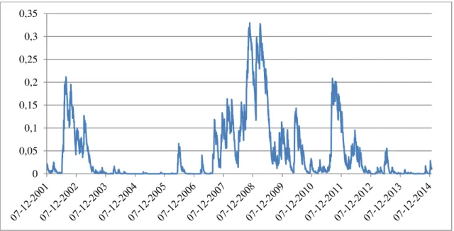
Figure 1 shows the composite index movements over the sample period. Being a sum of
market capitalizations it shows the overall UK financial sector performance during the crisis. The period from June 2007 until February 2009 then could be used as a crisis
period sample. Figure 2 shows the conditional probability (since there are conditional variances in it) of the one-day market loss of -1.6 times standard deviation or bigger.
During the crisis period it is obviously high because of the higher uncertainty level and, consequently, the higher volatility in the market.
Table 1 shows the main characteristics of the overall sample. As expected, the most
volatile and levered industry has the highest MES, according to all 3 types of MES (British Pound based MES, US Dollar based MES and US Dollar based GMES for
benchmarking). MES shows that the Life Insurance Sector has the biggest risk exposure at the end of 2014. The second risky sector is banking: it has the second highest average MES and second highest financial leverage. Therefore, firms from both sectors are
expected to become the most fragile part of the UK financial system in case of a negative shock.
7For more details visit Engle’s website and V
14
Table 2reports the statistics of returns over the period of their extreme deviations from
historical expectations during the 2007-2009 financial crisis. Comparing with the statistics for all data points, it is obvious that the average MES during the crisis is higher, and the volatility of returns also reaches its peaks – the level of uncertainty is completely different from that in calmer periods.
4.2. Components of MES
The first step for MES estimation was the estimation of 78 TARCH models (77 for
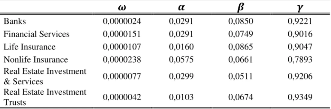
financial institutions’ returns and 1 for the composite index returns) to obtain estimates for and . Then, the median parameters were calculated for each sub industry.
Table 3(parameter )shows that there is less persistence of past shocks in conditional
variance for the firms in the group “Nonlife insurance”: the information obtained by the market at the last moment is more important for investors than past shocks. Also, for all
sub industry groups median level of is higher than the median level of . That means
more significant impact on variance at time coming from negative innovations, rather
than from past variance shocks itself.
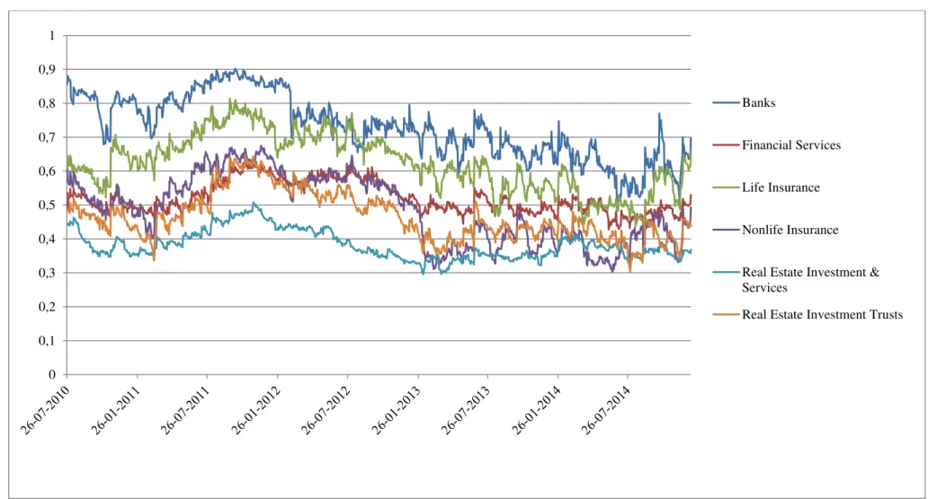
As discussed above, the main advantage of DCC models is to capture the time-varying behavior of relations between variables. Using dynamic conditional variances and
covariances (and, as a result, conditional correlations) allows us to build a time varying estimator of MES to observe its evolution across different industry groups. Figure 3
shows the evolution of dependence of each industry’s firms on the overall UK financial market movements (measured by conditional correlation). As expected, the more dependent an institution is on the overall industry, the more the systemic risk it takes: in
15
industries have the highest conditional correlations, so there is no surprise in obtaining
higher MES for them.
4.3. Behavior of MES by Sub Sectors
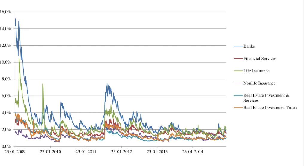
Figure 4presents the dynamic of MES since the beginning of 2009. Banks and Life
insurance specialized financial institutions have shown the highest fluctuation of risk exposure while other sectors were clustering under 4% level. The level of MES for
these two groups was always above the others’ level. Just after the recession, the banking sector attained a MES of 15% which meant 15% expected daily loss if the
industry loses percent. Generally, MES ranks of industry groups remained quite stable
over the given period of time.
4.4. Validity of MES estimates
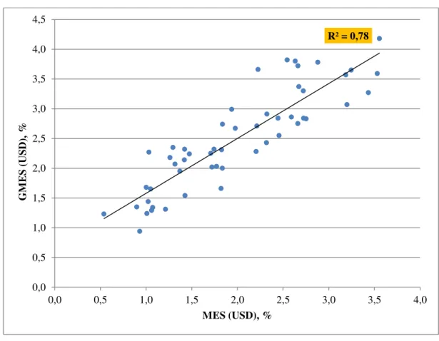
Comparing MES taken from the data in US Dollars with GMES, provided by the Volatility lab (See Figure 5), it may be concluded that MES estimates are valid, they
follow GMES by 78%. The difference (the remaining 22% of the MES variance) comes
from several factors, such as:
1. Different sample used. V-Lab took only 56 firms from the UK financial
industry. Since in this study there is the data for 77 firms, it affected (however,
not very significantly) the dynamics of the proxy for , and, as a result, the
dynamics of MES for all firms;
2. Different time frame. However the number of data points V-lab uses is not published, it is not likely that the number of data points used in this study is
16
3. Aggregation. V-Lab’s approach is more generalized and, actually, more sophisticated: they estimate MES for a particular firm regarding the relations with global market, not only the domestic;
4. Tails expectation. V-Lab’s MES are calculated using an assumption that innovation terms and are not independent – a special joint distribution for them – copula – was assumed. Consequently, the MES they obtained have this factor taken into account.
5. Forward-looking MES based on simulation. The V-Lab approach to estimate
LRMES is the following: with the information given at time simulate the
future outcomes and analyze “actual” statistics coming from such trials.
4.5. Currency Effects
As the data shows, the levels of MES estimated for any particular institution appeared to be dependent on the currency of the data used. Since (Brownless & Engle, 2010) use
generalized MES to compare firms across many countries against each other, a single currency was used – US Dollar, but following such methodology may lead to biases.
Although the British Pound and the US Dollar remain stable and solid currencies, their
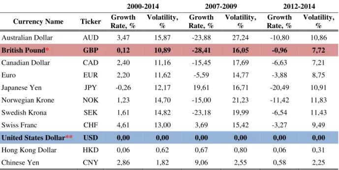
exchange rate is not constant, especially in crises. Among all the data points in the sample, the average annualized logarithmic return of USD-GBP pair is 0.12% with the volatility of 10.89%. Figure 6shows how significant shifts may be: during the year 2007
the British Pound lost almost 30% of its dollar price. Consequently, it affected MES estimates over the given sample. Other currencies’ statistics are reported in Table 4. The base currency is US dollar. Some of these currencies were affected by the financial crisis more than others: the highest loss is for British Pound while the Japanese Yen
17
Table 5 reports summary statistics on weighted aggregated MES, which are calculated
using different currencies with the same sample of UK financial institutions and time frame. As expected, they are different since currencies used differ: during the last three years MES in British Pounds is the highest, attaining 3.25%, while the lowest equals to
1.85% (for data in Australian Dollars). It is also interesting that during the crisis period the data in Japanese Yens has shown the highest MES, while the lowest “crisis” MES appeared again in Australian Dollars.
At first glance, there are no relationships between MES characteristics and currencies’ statistics. To check this, correlation coefficients (Spearman’s) between various
currencies’ statistics and MES descriptive statistics were calculated (see Table 6) for two sub-periods: “last-3-year” sample and “crisis” sample. For the first sample there are no coefficients with p-values lower than 20% except the correlation between average aggregated MES and its volatility: it could happen since MES captures volatility of returns and positively depends on it. For the second sample the data show lower MES
for higher volatility of the currency rate and higher MES for currencies gaining value in US Dollars during the crisis period. Regarding the size of the sample (only 10 data
points) taken for this exercise, it is not likely to be a robust result. Perhaps, for more currencies included more statistical evidence could be obtained.
Such results may appear also because of the following reason: since the model assumed
constant conditional expectations of returns (no any ARMA / ARIMA terms included) and demeaned returns were used for calculations, MES should be adjusted by including
for example an autoregressive model in the model specification. That, of course, would
affect estimations of ̂ and ̂ . Since it is quite feasible, that expected returns are
likely to fall during the crisis, it would be useful to allow ( ) and ( ) to be
18
5.
Conclusion
The 2007-2009 slumps gave a lot of information to be used in risk assessment – especially to predict (hopefully) the consequences of a negative market shock for a financial system. The intuitive and flexible (permitting many approaches to estimate its
indigents) MES concept has already gained reputation among researchers as a solid measurement of systemic risk. Being implemented to study the systemic risk in UK financial system, it reported the Life insurance and Banking sectors as weakest units of
the UK financial industry, corresponding to the GMES published by V-Lab.
Since this approach is widely used to compare systemic risk taken by financial firms in
different countries, currency effects may add a substantial level of noise, when data contains some firms with Market Cap, Liabilities and Equity appearing in non-domestic currencies. Consequently, MES estimates may be affected by these noisy currency
shifts. The analysis of the model with the same sample but with 10 different currencies shows that differences in MES estimates appeared which are not feasible to be predicted
by currency statistics, however, the sample many be not sufficiently large for statistical inference in this case. Nevertheless, using a non-domestic currency for MES estimations
19
Figure 1: Composite index (sum of market capitalizations of all firms from the sample), in Millions GBP
Figure 2: Probability of market loss percent or more in a single day, estimated at the end of the day before. Normality of standardized market residuals assumed. Takes volatility influence in any given data point
0,0 100.000,0 200.000,0 300.000,0 400.000,0 500.000,0 600.000,0
20
Table 1: Return and Volatility are annualized average daily numbers, averaged in each group. MES (GBP) - estimated using data in British Pounds. MES (USD) - the same estimator, calculated for the data in US Dollars.
GMES - Volatility Lab data (year end 2014)
ICB Sector Name # of firms Sum of Market Cap, GBP M Return, % Volatility, % Leverage, times MES (GBP), % MES (USD), % GMES (USD), %
Banks 7 273.389,5 6,55 49,96 16,61 1,63 2,08 2,95
Financial
Services 25 63.776,2 20,33 49,65 5,96 1,54 1,92 2,83
Life
Insurance 10 95.311,1 -4,58 58,46 19,23 1,97 2,49 3,29
Nonlife
Insurance 11 25.580,0 14,09 35,38 2,40 1,03 1,41 1,85
Real Estate Investment & Services
10 11.976,0 16,41 56,11 0,99 0,87 1,18 1,68
Real Estate Investment Trusts
14 41.760,3 18,16 48,16 0,75 1,08 1,29 2,02
Grand
Total 77 511.793,3 14,05 49,35 6,55 1,36 1,72 2,49
Table 2: Descriptive stats of returns by industries over the crisis period (Jun 2007 - Feb 2009)
ICB Sector Name Return, % Volatility, % Leverage, times MES (GBP), % MES (USD), %
Banks -114,48 106,75 34,89 5,64 4,03
Financial Services -92,06 75,31 7,51 2,94 2,52
Life Insurance -98,84 80,86 24,65 4,78 2,93
Nonlife Insurance -24,35 51,42 2,43 2,25 1,64
Real Estate Investment & Services
-173,72 80,23 3,24 2,85 2,28
Real Estate
Investment Trusts -140,13 61,90 0,92 2,66 2,62
Average -107,26 76,08 12,28 3,52 2,67
Table 3: Medians of 77 TARCH parameters for each financial institution grouped by industries
Banks 0,0000024 0,0291 0,0850 0,9221
Financial Services 0,0000151 0,0291 0,0749 0,9016
Life Insurance 0,0000107 0,0160 0,0865 0,9047
Nonlife Insurance 0,0000238 0,0575 0,0661 0,7893
Real Estate Investment
& Services 0,0000077 0,0299 0,0511 0,9206
Real Estate Investment
Figure 3: Average conditional correlations with market returns by industry groups
0 0,1 0,2 0,3 0,4 0,5 0,6 0,7 0,8 0,9 1
Banks
Financial Services
Life Insurance
Nonlife Insurance
Real Estate Investment & Services
22
Figure 4: Average MES by sub sectors.
0,0% 2,0% 4,0% 6,0% 8,0% 10,0% 12,0% 14,0% 16,0%
23-01-2009 23-01-2010 23-01-2011 23-01-2012 23-01-2013 23-01-2014
Banks
Financial Services
Life Insurance
Nonlife Insurance
Real Estate Investment & Services
23
Figure 5: MES (USD) and GMES by V-Lab compared
Figure 6: USD per 1 GBP currency ratio
R² = 0,78
0,0 0,5 1,0 1,5 2,0 2,5 3,0 3,5 4,0 4,5
0,0 0,5 1,0 1,5 2,0 2,5 3,0 3,5 4,0
G
M
E
S (
USD)
,
%
MES (USD), %
24
Table 4: Summary statistics of logarithmic daily growth rates for 10 world's major currencies: 2000-2014 - over the full sample; 2007-2009 - over the financial crisis period Jun'07-Feb'09; 2012-2014 - for last 3 years. *British Pound is
the domestic currency. **US Dollar is the base currency for this data
2000-2014 2007-2009 2012-2014
Currency Name Ticker Growth Rate, % Volatility, % Growth Rate, % Volatility, % Growth Rate, % Volatility, %
Australian Dollar AUD 3,47 15,87 -23,88 27,24 -10,80 10,86
British Pound* GBP 0,12 10,89 -28,41 16,05 -0,96 7,72
Canadian Dollar CAD 2,40 11,16 -15,45 17,69 -6,63 7,21
Euro EUR 2,20 11,62 -5,59 14,77 -3,88 8,75
Japanese Yen JPY -0,26 12,17 19,61 16,71 -20,49 10,91
Norwegian Krone NOK 1,23 14,70 -15,00 21,23 -11,42 11,83
Swedish Krona SEK 1,61 14,82 -23,18 19,99 -6,54 11,43
Swiss Franc CHF 4,61 13,00 3,69 15,42 -3,27 9,49
United States Dollar** USD 0,00 0,00 0,00 0,00 0,00 0,00
Hong Kong Dollar HKD 0,06 0,62 0,67 0,80 0,06 0,31
Chinese Yen CNY 2,86 1,82 9,06 2,55 0,58 2,25
Table 5:Summary statistics of weighted aggregated UK MES estimated using data in different currencies.
2007-2009 is the crisis period: from Jun’07 until Feb’09.*British Pound is the domestic currency. **US Dollar is the base currency for this data
2007-2009 2012-2014
Currency Used for MES estimations Agg MES average, % Agg MES Volatility, % Agg MES average, % Agg MES Volatility, %
Australian Dollar 3,39 1,42 1,85 0,35
British Pound* 4,83 1,85 3,25 0,67
Canadian Dollar 3,87 1,81 2,07 0,46
Euro 4,10 2,03 2,03 0,46
Japanese Yen 5,08 2,83 2,63 0,69
Norwegian Krone 3,80 1,73 1,89 0,43
Swedish Krona 4,00 1,87 2,07 0,43
Swiss Franc 4,58 2,11 2,04 0,46
United States Dollar** 4,48 2,19 2,51 0,66
Hong Kong Dollar 4,48 2,54 2,19 0,67
25
Table 6: Rank Spearman Correlations of MES (aggregated and averaged for the given time frame) and currencies’ summary statistics, grey items – do not have any interpretation regarding the scope of the study, items in bold – do.
10 different MES estimations (each per one currency) were used
2012-2014
Rate, % Growth
Volatility, %
Agg MES average, %
Agg MES Volatility, %
Growth Rate, % 1,00
Volatility, % -0,71 1,00
Agg MES average, % 0,39 -0,45 1,00
Agg MES Volatility, % 0,36 -0,51 0,74* 1,00
2007-2009
Rate, % Growth Volatility, % average, % Agg MES Volatility, % Agg MES
Growth Rate, % 1,00
Volatility, % -0,55 1,00
Agg MES average, % 0,55* -0,54* 1,00
Agg MES Volatility, % 0,85** -0,74** 0,80** 1,00
*p-value is less than 10%
26
Bibliography
Acerbi, C. & Tasche, D., 2001. "Expected Shortfall: a Natural Coherent Alternative to Value at Risk". Wilmott Magazine.
Acharya, V. V., Pedersen, L. H., Phillipon, T. & Richardson, M., 2010. "Measuring Systemic Risk", Cleveland: Federal Reserve Bank of Cleveland.
Adrian, T. & Brunnermeier, M. K., 2008. "CoVaR". Federal Reserve Bank of New York Staff Reports.
Baba, Y., Engle, R. F., Kraft, D. F. & Kroner, K. F., 1991. "Multivariate Simultaneous Generalized ARCH". University of Arizona.
Brownless, C. T. & Engle, R., 2010. "Volatility, Correlation and Tails for Systemic Risk Measurement". New York University - Stern School of Business.
Corvasce, G., 2013. "Measuring Systemic Risk: An International Framework". Society for Financial Studies.
Engle, R., 2002. "Dynamic conditional correlation: A simple class of multivariate GARCH models". Forthcoming Journal of Business and Economic Statistics.
Engle, R., Jondeau, E. & Rockinger, M., 2014. "Systemic Risk in Europe". Forthcoming in the Review of Finance.
Galati, G. & Moessner, R., 2013. "Macroprudential Policy: a Literature Review". Journal of Economic Surveys.
Scaillet, O., 2005. "Nonparametric Estimation of Conditional Expected Shortfall". Insurance and Risk Management Journal.