FEDERAL UNIVERSITY OF S ˜
AO CARLOS
CENTER FOR SCIENCE AND TECHNOLOGY
GRADUATE PROGRAM IN PHYSICS
QUANTUM MEMORY BASED ON ELECTROMAGNETICALLY
INDUCED TRANSPARENCY IN OPTICAL CAVITIES
ROMMEL RODRIGUES DE OLIVEIRA
FEDERAL UNIVERSITY OF S ˜
AO CARLOS
CENTER FOR SCIENCE AND TECHNOLOGY
GRADUATE PROGRAM IN PHYSICS
QUANTUM MEMORY BASED ON ELECTROMAGNETICALLY
INDUCED TRANSPARENCY IN OPTICAL CAVITIES
ROMMEL RODRIGUES DE OLIVEIRA
Dissertation submitted to the Graduate Program in Physics of the Federal University of S˜ao Carlos as part of the requirements for obtaining the title of Master in Physics.
Supervisor: Prof. Dr. Celso Jorge Villas-Bˆoas
Ficha catalográfica elaborada pelo DePT da Biblioteca Comunitária da UFSCar
O48qm
Oliveira, Rommel Rodrigues de.
Quantum memory based on electromagnetically induced transparency in optical cavities / Rommel Rodrigues de Oliveira. -- São Carlos : UFSCar, 2015.
52 f.
Dissertação (Mestrado) -- Universidade Federal de São Carlos, 2015.
1. Óptica quântica. 2. Informação quântica. 3. Computação quântica. I. Título.
Dedication
“If you’re gonna do something, do it right. You don’t always have to be the number one, but always give your best to be one of the greatest.”
Acknowledgments
First of all, I would like to thank my parents, Luiz Carlos de Oliveira and Soraia Rodrigues de Oliveira. For all the support they gave me through the years, for inspiring me to always aim high and dream big, for teaching me the value of hard work and education, and for all the sacrifices they made for me and my brothers so we could have a better life than theirs. They are true heroes, my best friends, and the best parents anyone could wish for and that I love with all my heart. A heartfelt thanks also goes to both my grandmothers, Maria Marlene Louren¸co and Marlene Candida de Oliveira whose I couldn’t be more grateful to have present in my life. And a specially sincere thanks to my late maternal grandfather, Jacob Rodrigues, my late paternal great-grandparents, Luzia Candida de Jesus and Henrique Gon¸cales, and my late maternal great-grandfather, Francisco Louren¸co Dias, who’ve always believed in me and I wished were here for this moment.
I would also like to thank Renato Molina Toth, a friend for several years now, and C´esar Rodrigues de Oliveira, my brother and friend since he was born, for sharing both aspirations and frustrations, and several glasses of beer, making this journey way easier with the company of those two. A special thanks also goes to Aparecido Marandola Jr., a personal friend and friend of the family who is always there, for good and bad times. And I shouldn’t forget to mention my youngest brother, Maur´ıcio Rodrigues de Oliveira, who is still young and I’m sure still has wonderful things reserved in his future.
A very special thanks goes to my supervisor, Prof. Dr. Celso Jorge Villas-Bˆoas. I’ve been working with him for several years now, and I have nothing but to thank him for. Everything I know about research in physics I’ve learned with him, who took the time and patience to teach me everything he could. All my accomplishments in this field are due to the special care he took with me when I was just a young undergrad student aspiring for a career in physics.
I would also like to thank my friend and work colleague Prof. Dr. James Alves de Souza for all conversations, both physics and non-physics related, and for making the work environment at the university a better place to be. A special thanks also goes to Mariana Vict´oria Ballottin, a very special friend inside and outside the physics department, whose company kept me sane during the hard times and kept me joyful during the happy ones.
I would also like to thank Prof. Rempe’s group, for hosting me and Prof. Celso for a week in their facilities during the final stage of this thesis, whose fruitful discussions provided amazing insights on our final results.
Technology of Quantum Information (INCT-IQ) for providing me with financial support for traveling expenses related to my research.
Abstract
Recently a quantum memory for a coherent pulse was accomplished using an atom trapped inside a high finesse cavity, where an efficiency of 9.3% was achieved for a storage time of 2µs and an average fidelity of 93% for a storage time of 180µs. We theoretically studied this system using the master equation approach, exhausting all the possible ways one could improve the efficiency, defined here as the ratio between the mean number of photons retrieved after the memory process and the mean number of photons that enters the empty cavity, η = ha†ai
out/ha†aiin, which proved to have an upper bound of 25%. Since protocols relying
Resumo
Recentemente uma mem´oria quˆantica para um pulso coerente foi realizada utilizando um ´atomo aprisionado em uma cavidade de alta finesse, onde uma eficiˆencia de 9.3% foi alcan¸cada para um tempo de armazenamento de 2µs e uma fidelidade m´edia de 93% para um tempo de ar-mazenamento de 180µs. Esse sistema foi estudado teoricamente utilizando a abordagem da equa¸c˜ao mestra, exaustando todos os poss´ıveis m´etodos para melhorar a eficiˆencia, definida aqui como a raz˜ao entre o n´umero m´edio de f´otons recuperados depois do processo da mem´oria e o n´umero m´edio de f´otons que entra na cavidade vazia, η=ha†ai
out/ha†aiin, que mostrou ter
Table of Contents
1 Introduction 11
2 Electromagnetically induced transparency 13
2.1 Jaynes-Cummings model . . . 13
2.2 EIT in free space . . . 14
2.3 EIT in optical cavities . . . 17
3 Quantum memory 20 3.1 Basic principles . . . 21
3.2 Master equation description . . . 23
4 Results 24 4.1 Simulating the Experiment . . . 24
4.2 Optimizing the efficiency . . . 26
4.2.1 Optimizing the efficiency as a function of ΩC . . . 26
4.2.2 Optimizing the efficiency as a function ofζ . . . 26
4.2.3 Optimizing the efficiency as a function oft1 . . . 27
4.2.4 Optimizing the efficiency as a function ofg . . . 29
4.2.5 Optimizing the efficiency as a function of the number of atoms . . . 33
4.3 Reflection and transmission losses . . . 37
4.4 Single photon input . . . 38
4.5 Input-output theory with phase-matching condition . . . 42
4.6 Revisiting the relation between the field inside and outside the cavity . . . 43
4.7 The role of the phase-matching condition in the memory efficiency . . . 46
4.8 Choosing the adequate setup . . . 47
5 Conclusions 49
Chapter 1
Introduction
With the growing improvement of computer’s processing power, Gordon Moore, Intel’s co-founder, made a prediction: the computing power will double, maintaining a constant price, approximately every two years. This means that every couple of years the number of transistors in a processor will double, which implies in reducing the size of a transistor so that it is possible to fit twice as many of them in the same space as before. This prediction became known as Moore’s Law.
Transistors are inherently quantum, i.e., their behavior can only be explained with the laws of quantum mechanics, although in a classical circuit they only work as a valve. Nevertheless, Moore’s Law establishes a limit for how small a transistor can be. Thus, it is necessary to seek another way to increase computing power, that is not by increasing the number of transistors. At this point enters quantum computation.
In the 1980s, the research field of quantum computation starts to take shape. Analogously to the Turing machine, in 1985 David Deutsch proposes an universal quantum computer, a model in which the operations and the algorithms’ logic are based on the principles of quantum mechanics [1].
In classical computation the information is coded in a binary system. The smallest unit of information is the bit, and it can take two values: 0 or 1. Hence, in a system with n bits, n pieces of information are required to determine a certain state: if each one of the n bits is either on (1) or off (0). In quantum computation, in addition to the states that are encountered in classical computation, the quantum bits, or qubits, can assume any superposition between the classical states, so that for a system withn qubits, 2npieces of information are required to
completely describe a state [1]. Forn= 500, 2500is greater than the estimated number of atoms
in the universe. The goal of quantum computation is to use this amount of information that quantum systems are able to manipulate, to create faster and more efficient algorithms than their classical analogues, or even perform tasks that before were impossible, such as simulate more complex quantum systems [2].
CHAPTER 1. INTRODUCTION 12
An essential element for quantum computation is a quantum memory [3]. This device can be defined as a system capable of storing quantum states to perform a certain task. Quantum memories can be applied not only in quantum computation but also in quantum repeaters, metrology, detection and emission of single photons, and as a system to study fundamental aspects of quantum mechanics [4]. Among the physical systems used to its implementation are solid state atomic ensembles, nitrogen vacancy centers, quantum dots, systems with a single atom, quantum gases and optical phonons in diamond [5].
Here a system composed of a single atom trapped in an optical cavity stores an input state in the atom’s electronic levels by means of the electromagnetically induced transparency (EIT). Recently a quantum memory was accomplished using this system, where an efficiency of 9.3% was achieved for a storage time of 2µs and an average fidelity of 93% for a storage time of 180µs[6]. It is interesting to optimize the storage efficiency of this system for applications such as quantum repeaters, which may require the efficiency to be greater than 90% [4], and linear optical quantum computation, which may require an efficiency above 99% [4].
Chapter 2
Electromagnetically induced
transparency
In this chapter we will briefly present the theoretical background needed for understanding cavity EIT. We begin with the Jaynes-Cummings model, that describes a coherent energy exchange between atom and field. Afterwards we present the basics aspects of EIT in free space. Finally, EIT in optical cavities is introduced and briefly discussed.
2.1
Jaynes-Cummings model
The Jaynes-Cummings Hamiltonian, that describes a coherent energy exchange between atom and field is, in the Schr¨odinger picture, given by [9]
HJ C =~ω0σee+~ωa†a+~g(aσeg +a†σge). (2.1)
In this Hamiltonian ω0 and ω are respectively the atomic transition and the cavity mode
frequencies; g is the atom-field coupling (vacuum’s Rabi frequency); a (a†) is the annihilation
(creation) operator of the field; andσij =|iihj|, i, j =e, g, where |giis the atom’s ground state
and |ei is its excited state.
It is important to remember that two approximations were made to reach this model: the dipole approximation, valid when the wave length of the impinging radiation is large in comparison with the atomic radius, and the rotating wave approximation, that discards rapid oscillating terms that have a negligible contribution to the system’s dynamics, valid in the limit when the atom-field coupling is small in comparison to the characteristics frequencies of the system.
CHAPTER 2. ELECTROMAGNETICALLY INDUCED TRANSPARENCY 14
Figure 2.1: Diagram of levels involved in an usual EIT process.
2.2
EIT in free space
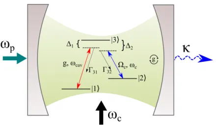
In this section we analyze the problem of an atomic sample that consists of 3 level atoms interacting with two classical fields. Levels |1i and |2i are the ground states, and there is no dipole transition between them. Level|3iis the excited state, and it can decay both to level|2i as well as to |1i. Interacting with the transition|1i ↔ |3i is a probe field with Rabi frequency ΩP and frequencyωP, and interacting with the transition|2i ↔ |3ithere is a control field with
Rabi frequency ΩC and frequency ωC. There is a detuning ∆1 between the frequencies of the
probe field and the transition |1i ↔ |3i, ω31, and a detuning ∆2 between the frequencies of
the control field and the transition |2i ↔ |3i, ω32. The polarization decay rate related to the
|1i ↔ |3i transition is Γ31 and the polarization decay rate related to the |2i ↔ |3i is Γ32. Such
setup is called Λ configuration and is illustrated in Figure 2.1.
Adopting |1i as our zero energy, the system’s HamiltonianH =H0+Hint is given by
H =ω3σ33+ω2σ22+{ΩP(t)σ31e−iωPt+ ΩC(t)σ32e−iωCt+h.c.}, (2.2)
where
H0 =ω3σ33+ω2σ22,
and
Hint={ΩP(t)σ31e−iωPt+ ΩC(t)σ32e−iωCt+h.c.}.
Here h.c. stands for hermitian conjugate, and σij = |iihj| (i, j = 1,2,3) are the atomic
operators that describe the level populations (i=j), and the transitions between them (i6=j). It is worth reminding that from this point on we use ~= 1 to simplify the notation.
Going to the interaction picture, through a unitary transformation U = e−iH0t, we have that the interaction Hamiltonian ˜HI, that describes the dynamics of two classical fields acting
on a atomic sample, is given by
˜
CHAPTER 2. ELECTROMAGNETICALLY INDUCED TRANSPARENCY 15
with ∆1 = ω31 −ωp (ω31 = ω3) and ∆2 = ω32 −ωc (ω32 = ω3 −ω2). Removing the time
dependency, through a unitary transformation, U =ei(∆1σ33−(∆2−∆1)σ22)t, the new Hamiltonian is given by
HI = ∆1σ33+ (∆1−∆2)σ22+ (ΩPσ31+ ΩCσ32+h.c.). (2.4)
Equation 2.4 has three eigenenergies and eigenstates. One of them is a dark state with a zero eigenenergy, λ0 = 0, which is given by
|Di=cosθ|1i −sinθ|2i, (2.5) where
tan(θ) = ΩP ΩC
.
To visualize the effects of the field on the atomic medium one must calculate the electric susceptibility of the medium. The polarization of a material medium is given by
~
P =χeE,~
where χe is the medium’s linear susceptibility, with
Re(χe)→medium’s dispersion,
Im(χe)→medium’s absorption.
The polarization can also be written as
~
P =X
i
h~µii
V = N
V T r(ρ~µ),
where N is the total number of atoms in the volume V and ρ is the density matrix of the system. Here we are working on the limit of low atomic densities, with non-interacting atoms. For a 3 level atom the most general density operator (in Schr¨odinger picture) can be written as
ρ=ρ11|1ih1|+ρ22|2ih2|+ρ33|3ih3|+ (ρ21e−iω21t|2ih1|+ρ31e−iω31t|3ih1|+ρ32e−iω32t|3ih2|+h.c.),
and the dipole moment operator is given by
~µ=~µ13|1ih3|+~µ23|2ih3|+h.c. .
Thus
~ P = N
V (~µ13ρ31e
−iω31t+~µ
CHAPTER 2. ELECTROMAGNETICALLY INDUCED TRANSPARENCY 16
The terms ρ31 and ρ32 and their complex conjugates may be obtained through the master
equation for this system [7]
dρ
dt =−i[HI, ρ] + Γ31(2σ13ρσ31−σ33ρ−ρσ33) + Γ32(2σ23ρσ32−σ33ρ−ρσ33) +γ2(2σ22ρσ22−σ22ρ−ρσ22) +γ3(2σ33ρσ33−σ33ρ−ρσ33),
(2.6)
where γ2 and γ3 are the dephasing rates of the levels 2 and 3.
Here HI is given by Equation 2.4. However it is important to remember that with the
Hamiltonian HI we are at the rotating frame and, once the solution is obtained, one must go
back to the Schr¨odinger picture. Knowing that
hi|ρ|ji ≡ρij and hi|ρ˙|ji ≡ρ˙ij,
taking the asymptotic limit, i.e., ˙ρij = 0, and the limit in which |ΩP| ≪ |ΩC|, that implies
ρ11 ≃ 1, ρ22 ≃ 0 and ρ33 ≃ 0, it is possible to obtain the elements of ρ. In the interaction
picture [10]
ρ31=
2iΩP[2γ21+ 2i(∆1−∆2)]
(2γ31+ 2i∆1)[2γ21+ 2i(∆1−∆2)] + 4Ω2C
ei∆1t and
ρ32= −
i8Ω2PΩCei∆2t
(2γ32+ 2i∆2){(2γ31−2i∆1)[2γ21−2i(∆1 −∆2)] + 4Ω2C}
,
whereγ31= Γ31+ Γ32+γ3,γ32= Γ31+ Γ32+γ3+γ2 andγ12 =γ2. Recalling that ∆1 =ω31−ωP
e ∆2 =ω32−ωC, and defining ∆≡∆1 and δ ≡∆1−∆2
~ P = N
V {~µ13
2iΩP[2γ21+ 2iδ]
(2γ31+ 2i∆)[2γ21+ 2iδ] + 4Ω2C
e−iωPt+c.c
−~µ23 −
8iΩ2
PΩCe−iωCt
(2γ32+ 2i(∆−δ)){(2γ31−2i∆)[2γ21−2iδ] + 4Ω2C}
+c.c},
with c.c. meaning the complex conjugate. On the other hand, P~ = χeE~ and E~ = E~Pe−iωPt+
~
ECe−iωCt+c.c. Since we are interested in the medium’s response to the probe field, we take
the term with e−iωPt and its complex conjugate. Therefore
χ(1)(−ωP, ωP) =
N
V |~µ13|2ΩP
i[2γ21+ 2iδ]
(2γ31+ 2i∆)[2γ21+ 2iδ] + 4Ω2C
, (2.7)
whose real part is given by
Re(χ(1)) = N
V |~µ13|2ΩP
2γ21[4γ31(∆−δ) + 4γ21∆] +δ[8∆δ−8Ω2C]
|(2γ31+ 2i∆)[2γ21+ 2iδ] + 4Ω2C|2
CHAPTER 2. ELECTROMAGNETICALLY INDUCED TRANSPARENCY 17
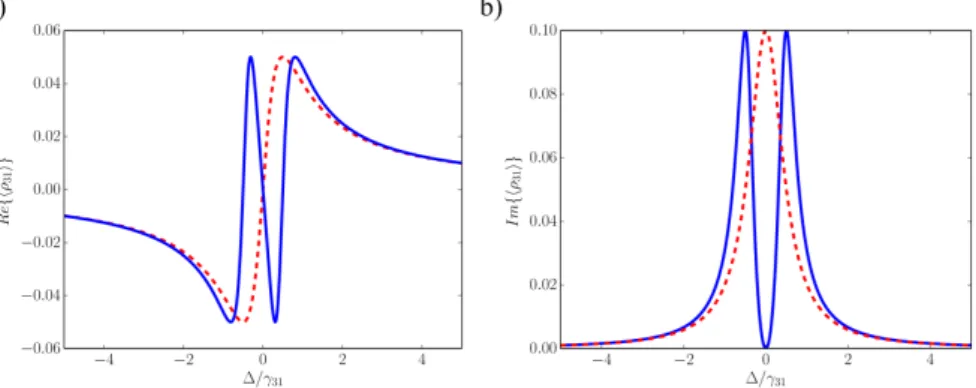
Figure 2.2: Electromagnetically induced transparency characteristic curves. In the blue solid curve the control field is on, while in the red dashed curve the control field is off. a) Real part of ρ31, which is proportional to the atomic medium’s dispersion. b) Imaginary part of ρ31, that
is proportional to the medium’s absorption. The values used here were: γ31= 1M Hz,γ21 = 0,
δ= 0, Ωp = 0.1γ31, and Ωc =γ31 in the blue solid curve and Ωc = 0 in the red dashed curve.
and its imaginary part by
Im(χ1) = N
V |~µ13|2ΩP
2γ31(4γ212 + 4δ2) + 8γ21Ω2C
|(2γ31+ 2i∆)[2γ21+ 2iδ] + 4Ω2C|2
. (2.9)
Figure 2.2 shows the real and imaginary parts of ρ31, for Ωc = 0 and Ωc 6= 0. The Equations
2.8 and 2.9 are proportional to the real and imaginary parts of ρ31, respectively.
We can see in Figure 2.2 a) the real part of ρ31, which is proportional to the medium’s
dispersion. When the control field is turned on, solid blue curve, one can see a rapid variation in the medium’s dispersion for a small change in the detuning. This will lead to the phenomenon of slow light, since the light’s velocity in a medium is inversely proportional to the derivative of the medium’s dispersion. Figure 2.2 b) shows the imaginary part of ρ31, which is proportional
to the medium’s absorption. In the solid blue curve, which depicts the situation when the control field is on, one can see the effect of turning the control field on: it creates a minimum in the absorption when the detuning is null, i.e., the medium is now transparent to the probe field when the control field is on. This is the basic principle of EIT, making a medium transparent to a certain wavelength by shining it with light of a different wavelength.
2.3
EIT in optical cavities
In this section a system consisting of a 3 level atom in the Λ configuration inside a high finesse cavity will be analyzed. The cavity mode, of frequencyω, interacts with the transition|1i ↔ |3i with a coupling rateg (Rabi frequency). Interacting with transition |2i ↔ |3ithere is a control field with Rabi frequency ΩC and frequency ωC. There is also a pumping in the cavity (probe
CHAPTER 2. ELECTROMAGNETICALLY INDUCED TRANSPARENCY 18
Figure 2.3: Electromagnetically induced transparency inside an optical cavity.
a way that an intense probe field impinges on the left cavity mirror, which has a very high reflectivity. Only a small portion of light is transmitted, and we calculate the interaction of it with the atom inside the cavity. The right mirror has a smaller reflectivity than the left one, so that light leaves the cavity preferably through the right side of it, where a detector is placed to make transmission measurements. This system is illustrated in Figure 2.3.
Setting |1ias zero energy, the system’s Hamiltonian is given by
H =ω3σ33+ω2σ22+ωa†a+ (gaσ31+ ΩCσ32e−iωCt+εaeiωpt+h.c.), (2.10)
where
H0 =ω3σ33+ω2σ22+ωa†a,
Hint = (gaσ31+ ΩCσ32e−iωCt+εaeiωpt+h.c.).
In the interaction picture, obtained through the unitary transformation U0 = e−iH0t, we
have
HI = (gaσ31ei∆1t+ ΩCσ32ei∆2t+εaei∆t+h.c.) , (2.11)
where
∆1 =ω3−ω: detuning between atom and cavity,
∆2 = (ω3−ω2)−ωC: detuning between atom and control field,
∆ = ωp−ω: detuning between probe field and cavity.
Taking the time dependency throughU1 =e−i[∆a
†a−∆
1σ33−(∆1−∆2)σ22−∆σ11]t, we get the Hamil-tonian [11]
CHAPTER 2. ELECTROMAGNETICALLY INDUCED TRANSPARENCY 19
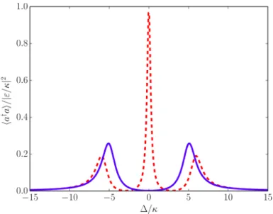
Figure 2.4: Normalized transmission (ha†ai/|ε/κ|2) as a function of the detuning between cavity
and probe field. The parameters used here wereκ= 1M Hz,g = 5κ, ΩC = 3κin the red dashed
curve and ΩC = 0 in the blue solid curve, Γ31 = 1κ, Γ32 = 0 , γ2 = 0, γ3 = 0, ∆1 = ∆2 = 0,
ε=√0.01κ.
The master equation for this system is given by
dρ
dt =−i[HI, ρ] +κ(2aρa
†
−a†aρ
−ρa†a)
+Γ31(2σ13ρσ31−σ33ρ−ρσ33) + Γ32(2σ23ρσ32−σ33ρ−ρσ33)
+γ2(2σ22ρσ22−σ22ρ−ρσ22) +γ3(2σ33ρσ33−σ33ρ−ρσ33)
(2.13)
where κ is the cavity field decay rate, Γ32 and Γ31 are the polarization decay rates related to
the |2i ↔ |3i and to the |1i ↔ |3i transitions, respectively, and γ2 and γ3 are the dephasing
rates of the levels 2 and 3, respectively. Figure 2.4 shows the normalized transmission from the cavity, obtained through the master equation, when the control field is off and on, clearly showing the transparency window provided by the EIT. It is important to remember that the condition Γ32 = 0 used in this graph is a bit artificial. In reality Γ32 never is exactly null for a
three level atom, and graphs of this kind, for when the control field is off (red dashed curve), are only obtained by making measurements in a time when the system did not reach the full stationary state, and the atom can be considered as a two level system, i.e., Γ32 ≃0.
Chapter 3
Quantum memory
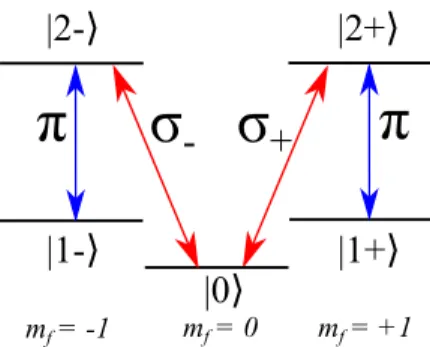
In this chapter we are going to explain the basic principles of a quantum memory and see the methods we are going to use to study it. It should be clear to the reader that, although here we are using a simpler version of the quantum memory, where the qubits are 0 and 1 photons, in the experiment [6] the qubits were implemented using polarization states, σ+ and σ−. Our
simplification should not affect the results, since the system used for the polarization states can be seen as two three level systems, as it can be seen in Figure 3.1. It should also be clear the difference we are making between single sided and two sided cavities. In a single sided cavity, we probe it through the less reflective mirror and measure the outcome through the same side. In a two sided cavity, we probe the cavity through the more reflective mirror and measure the outcome through the less reflective one. Cavity EIT is done with a two sided cavity, and since we are studying a memory based on cavity EIT, our model will also consist of a two sided cavity.
|1-
⟩
|1+
⟩
|2+
⟩
|2-
⟩
|0
⟩
σ
+
σ
-π
π
mf = -1 mf = 0 mf = +1
Figure 3.1: 5 level atom diagram. Here we have three ground states, | −1i,|0i and |+ 1i, and two excited states, | −2i and |+ 2i. The control field, with linear polarized light, couples the transitions| −1i ↔ | −2iand|+ 1i ↔ |+ 2i. The cavity, with circularly polarized light couples the transitions |0i ↔ |+ 2i and |0i ↔ | −2i. This structure is symmetric, and can be seen as two three level atoms.
CHAPTER 3. QUANTUM MEMORY 21
3.1
Basic principles
The main objective of this work was to study the storage and recovery process in an optical quantum memory based on cavity EIT, as accomplished in [6], so that the efficiency of the device be optimized, within the available experimental conditions. The efficiency is defined as the ratio between the mean number of photons retrieved after the memory process and the mean number of photons that enters the empty cavity, i.e., η=ha†ai
out/ha†aiin.
The principle behind EIT based quantum memories is to use the transparency window generated by the phenomenon. For an ensemble of atoms, first one must prepare them in the ground state |1iwhich, in the limit where Ωc ≫Ωp, is a dark-state of the system. If instead of
a probe field, a pulse with one photon is sent, with frequency spectrum within the transparency window, with the control field on this pulse is not absorbed. However, if one adiabatically turns off the control field, keeping the system in the dark-state, the pulse is now absorbed and the dark-state is now |2i.
Similarly, if the efficiency of the process is high enough, one can send a pulse with a superpo-sition of 0 and 1 photon. Adiabatically turning off the control field will store this superposuperpo-sition in the atomic levels.
For a single atom in a cavity, when the field has at most one excitation, the dark-state is, according to Equation 2.12, given by [12]
|Di=−iΩc|1iatom|1ipf ield−g|2iatom|0if ield Ω2
c +g2
.
If Ωc ≫g⇒ |Di ≃ |1iatom|1if ield. If Ωc ≪g⇒ |Di ≃ |2iatom|0if ield. Therefore, if the initial
state is|ψ(0)i=|1iatom|1if ield, and Ωc ≫g, turning off the control field adiabatically, according
to the adiabatic theorem [13], the system will remain in the dark state which eventually will be |ψ(tf inal)i=|2iatom|0if ield
Below we have an example of how this would work. Consider an initial state for the light given by
|ψi=α|0if ield+β|1if ield.
So now we have
(α|0if ield+β|1if ield)|1iatom =α|0if ield|1iatom+β|1if ield|1iatom.
Adiabatically turning off the control field, the atom can absorb one excitation of the field, thus
α|0if ield|1iatom+β|1if ield|1iatom
(Ωc→0)
−→
CHAPTER 3. QUANTUM MEMORY 22
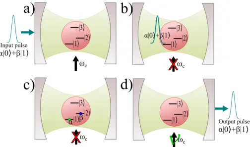
Figure 3.2: Scheme of a quantum memory based on cavity EIT. a) Input pulse with a state that is a superposition of 0 and 1 photon impinges the cavity, which is coupled to the |3i ←→ |1i transition. The atom is initially in the state |1i and has a control field coupling the transition
|3i ←→ |2i. b) When the pulse enters the cavity, the control field is turned off so that the
transparency window closes. c) With the control field off, the atom absorbs the field excitation, transferring its superposition to the atomic ground states. d) To recover the stored state, the control field is turned back on, the atom coherently emits the light, maintaining its initial superposition if none logical operation is performed in the atom during the storage period.
Finally
|ψf inali=α|0if ield|1iatom+β|0if ield|2iatom =|0if ield(α|1iatom+β|2iatom).
That is, the initial state of light, a superposition of 0 and 1 photon, is transferred to an atomic state, a superposition of the ground states of the atom |1i e |2i.
Once the state is stored in the atom, one can recover it after a storage time, simply by adiabatically turning the control field back on. The storage time is limited by decoherence effects [6], however, it should be clear that here we are not taking this into account. The storage time can be limited by the dephasing of the electronic states, γ2 and γ3, but here we
consider them null in such a way that the efficiency is does not become lower for a longer storage time, i.e., the storage time does not play a role in the efficiency in our simulations, although including these effects is trivial.
CHAPTER 3. QUANTUM MEMORY 23
3.2
Master equation description
The master equation formalism is the same introduced when the electromagnetically induced transparency was discussed. As it was shown before, the dynamics of a single three-level atom in the Λ configuration trapped in an optical cavity is governed by the master equation 2.13.
Here, however, we are going to work with all the detunings being null. So, finally, we have this simple form of the Hamiltonian
HI = (εa+ε∗a†) + (gaσ31+ga†σ13) + [ΩCσ32+ Ω∗Cσ23]. (3.1)
Now, if we want to use this model to describe a quantum memory made up of this system, we have to make a few alterations in our Hamiltonian. First, the pump field is no longer an always turned on field, instead we are going to give it a Gaussian dependency in time
ε(t) = Eme−
1 2
(t−t0)2
α2 . (3.2)
This probe field is what we are interested in storing in the atom. To do so, we also must turn off the control field, making the atom absorb the probe, and we also have to turn the control field back on so we can restore the probe field stored in the atom. We do this by giving a time dependency to the control field of the form
ΩC(t) = ΩM AXC
1
2{[1−tanh(ζ1(t−t1))] + [1 +tanh(ζ2(t−t2))]}, (3.3) where ζ1 controls the rate at which we turn off the control field and ζ2 controls the rate at
Chapter 4
Results
In this chapter we show and discuss our results for a quantum memory based on cavity EIT. First, we simulate the experiment done by H. P. Specht et al. [6]. Once that is done, we begin our optimization of the efficiency. For this end, we select one parameter to vary and lock all other parameters. We begin with the maximum amplitude of the control field ΩM AX
C . Next, we
investigate ζ, that controls the velocity by which we turn off and on the control field. In the following, we study the dependency of the efficiency ont1, the time chosen to turn off the control
field. This is done by fixing a value for the time t0 when the input pulse has its maximum,
and varying t1. Afterwards, the dependency of the efficiency on the atom-field coupling g is
investigated. In this part are shown curves for the efficiency as a function of g, for selected values of the full width at half maximum (FWHM) of the input pulse, as well as different values of its amplitude ε, which has to be sufficiently small so that the probability of two or more photons inside the cavity is null. Lastly, the efficiency as a function of the number of atoms is investigated. After the optimization, a discussion on reflection and transmission losses is made, and seen as the main reason for the limitation of the efficiency in our current model. Next, using an approach developed by H. Carmichael [14], a quantum memory is simulated for a single photon input, and through a small modification we also simulate for a weak coherent pulse input. Due to the results obtained, we turn our attention to an input-output theory and revisit the relation between the field inside and outside the cavity. A small discussion on the role of phase-matching conditions on the memory efficiency is made, followed by a discussion on the right choice of the experimental setup. It’s worth mentioning that all the figures in this document were obtained with simulations using the Quantum Toolbox in Python (QuTiP) [15].
4.1
Simulating the Experiment
Our first step, now that we have our model ready, is to try and reproduce the experiment of the single atom quantum memory [6] with ours simulations.
CHAPTER 4. RESULTS 25
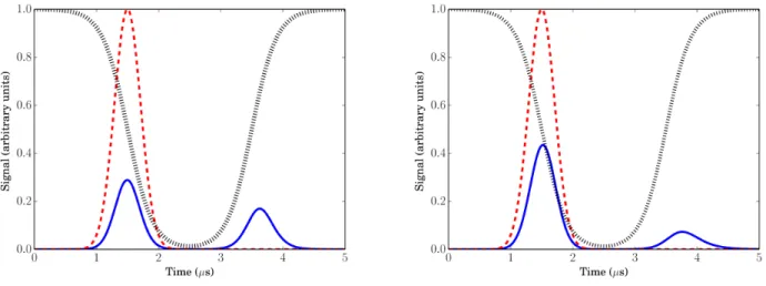
Figure 4.1: Single atom quantum memory scheme. The control field ΩC, black dotted curve,
is initially at its maximum value. Then we send in the input pulse ε, red dashed curve, at which point we slowly turn off the control field. The solid blue curve shows the mean number of photons in the cavity, and as the control field is turned off, the photons are absorbed by the atom. Later on, when we want to recover the pulse, we simply turn the control field back on. The parameters used here were: κ/2π = 2.5MHz, g = 2.0κ in the left and g = 1.09κ in the right, ΩM AX
C = 2g/3, EM =
√
10−4κ, ζ
1 = ζ2 = ζ = 1.5MHz, and F W HM = 1.0µs. We
obtained an efficiency of 17.49%
In Figure 4.1 a) we try to use the same parameters mentioned in the reference [6]. The result is that we obtained an efficiency of 17.49%, which is almost twice as much as the 9.3% value of the experiment.
So, what’s wrong with our model? The first thing we can point out is that we don’t take into account oscillations of the atom in the cavity, i.e., we don’t consider any deviations in the value of the coupling constantg. In real experiments the atom moves inside the cavity, leading to a time dependent atom-field coupling, which is sometimes close to its maximum value, but also occasionally close to its minimum one. Another effect of the motion of the atom in the cavity is that it experiences different stark shifts in the dipole trap. Due to this, an exact value of the atomic resonance is not possible to be known.
CHAPTER 4. RESULTS 26
0.0 0.5 1.0 1.5 2.0
ΩC/ g
0.00 0.05 0.10 0.15 0.20 0.25
Efficienc
y
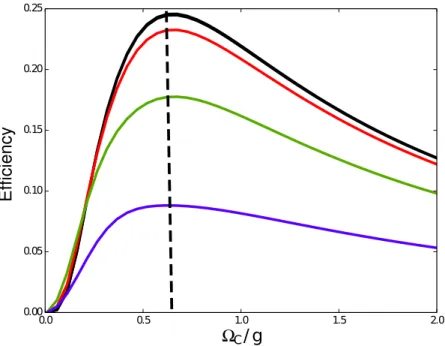
Figure 4.2: Efficiency in function of ΩM AX
C . The parameters used here were: κ/2π= 2.5M Hz,
Γ31= Γ32= 0.6κ,ζ1 =ζ2 = 1.9M Hz,EM =
√
10−4κ,F W HM = 1.0µsandg = 1κin the blue
curve, g = 2κ in the green curve, g = 5κ in the red curve and g = 15κ in the black curve.
4.2
Optimizing the efficiency
4.2.1
Optimizing the efficiency as a function of
Ω
CHere we investigate what’s the dependency of the efficiency on the maximum value of the control field ΩM AX
C , for different values of g. It is important to stress that throughout the
optimizations made, unless said otherwise, an input pulse with a fixed intensity and full width at half maximum was used.
In Figure 4.2 we see that for all values of g, we have a peak in the efficiency around ΩM AX
C = 0.6g and ΩM AXC = 0.7g. The behavior exhibited in this graph is due to the fact that
the width of the frequency window in the EIT transmission spectrum for this system depends both on ΩC and g. So, from now on, we are going to fix the value of ΩM AXC at 2g/3.
4.2.2
Optimizing the efficiency as a function of
ζ
Other parameters that could have an import role in the efficiency areζ1 andζ2, that determine
how fast we turn off and on the control field.
First we are going to say that ζ1 = ζ2 = ζ, and we investigate how the overall efficiency
CHAPTER 4. RESULTS 27
0 1 2 3 4 5
ζ(M Hz) 0.00
0.05 0.10 0.15 0.20 0.25
E
ffi
c
ie
n
c
y
Figure 4.3: Efficiency as a function of ζ1 = ζ2 = ζ. The parameters used here were: κ/2π =
2.5M Hz, Γ31 = Γ32 = 0.6κ, ΩM AXC = 2g/3, EM =
√
10−4κ, F W HM = 1.0µs and g = 1κ in
the blue curve, g = 2κ in the green curve, g = 5κ in the red curve and g = 15κ in the black curve.
Now we are going to look how ζ1 and ζ2 separately affect the efficiency. First we see the
dependency of the efficiency on ζ1.
Figure 4.4 a) show us a very similar dependency of the efficiency on ζ1 to the dependency
of the overall efficiency on ζ. Moreover the peak is in the same point, ζ1 = 1.75M Hz.
In Figure 4.4 b) we plot the dependency of the efficiency on the parameter ζ2. Unlikeζ1,ζ2
shows little effect on the efficiency for sufficiently large ζ2, and for the greater the value of the
coupling constant, smaller is the impact of ζ2 on the efficiency.
From now on we fix the values of ζ1 and ζ2 at 1.75M Hz.
4.2.3
Optimizing the efficiency as a function of
t
1Another parameter that could influence the efficiency is the time we choose to turn off the control field relatively to the time the pulse enters the cavity.
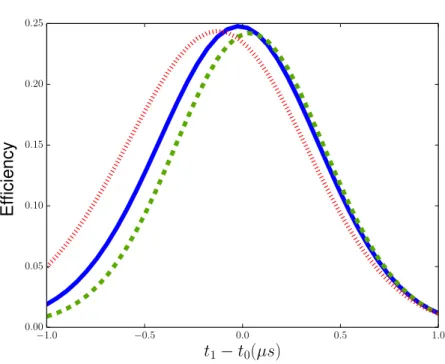
Figure 4.5 show us indeed that when the difference between the center of the probe field pulse, t0, and the time we choose to turn off the control field, t1, is null, we have the best
efficiency. One should also notice that if the parameter ζ =ζ1 =ζ2 is changed, the best value
CHAPTER 4. RESULTS 28
0 1 2 3 4 5
ζ1(M Hz)
0.00
0.05
0.10
0.15
0.20
0.25
E ffi c ie n c y
0 1 2 3 4 5
ζ2(M Hz)
0.00
0.05
0.10
0.15
0.20
0.25
E ffi c ie n c y
Figure 4.4: Efficiency in function of ζ1 on the left and as a function of ζ2 on the right. The
parameters used here were: κ/2π = 2.5M Hz, Γ31= Γ32= 0.6κ, ΩM AXC = 2g/3,EM =
√
10−4κ,
F W HM = 1.0µs and g = 1κ in the blue curve, g = 2κ in the green curve, g = 5κ in the red curve and g = 15κ in the black curve.
−1.0 −0.5 0.0 0.5 1.0
t1−t0(µs)
0.00 0.05 0.10 0.15 0.20 0.25
E ffi c ie n c y
Figure 4.5: Efficiency as a function oft1−t0. The parameters used here were: κ/2π= 2.5M Hz,
Γ31 = Γ32 = 0.6κ, ΩM AXC = 2g/3, EM =
√
10−4κ, F W HM = 1.0µs,ζ = 1.25M Hz (red dotted
CHAPTER 4. RESULTS 29
0 5 10 15 20
g/κ
0.0
0.2
0.4
0.6
0.8
1.0
R e c o v e ry E ffi c ie n c y
Figure 4.6: Recovery efficiency as a function of g (left) and single photon generation efficiency from the reference [17] (right). The parameters used on the left figure were: κ/2π= 2.5M Hz, Γ31= Γ32= 0.6κ, ΩM AXC = 2g/3, EM =
√
10−4κ, F W HM = 1.0µsand ζ = 1.75M Hz.
4.2.4
Optimizing the efficiency as a function of
g
Finally, we now investigate how the efficiency is affected by the coupling constant g.
First, lets look at how the coupling g affects the recovering efficiency. We define the recov-ering efficiency as the ratio between what the atom emits divided by what the atom absorbs.
Figure 4.6 a) show us that for sufficiently large g, the recovering efficiency tends to 100%. It is clear that for a sufficiently high coupling the recovery efficiency reaches 100%. A similar situation is shown in figure 4.6 b), taken from reference [17], where the single photon generation efficiency is studied. In the former case, the single photon generation efficiency also reaches values close to 100% for sufficiently high atom-field coupling. In both cases what is being studied is the ability of transferring the atom excitation to the field mode, and, as expected, both cases show similar results.
Now, lets look at the dependency of the efficiency, what the atom emits divided by what we sent to the cavity, on the coupling g.
Figure 4.7 show us that for this set of parameters, the efficiency saturates at about 25%, no matter how large g is.
However, as we said, this is the case for this set of parameters. What would happen if we changed things a little? Perhaps there is some parameter that is limiting the efficiency.
For different values of ε
CHAPTER 4. RESULTS 30
0 5 10 15 20
g/κ
0.00 0.05 0.10 0.15 0.20 0.25
E
ffi
c
ie
n
c
y
Figure 4.7: Efficiency as a function of g. The parameters used here were: κ/2π = 2.5M Hz, Γ31= Γ32= 0.6κ, ΩM AXC = 2g/3, EM =
√
10−4κ, F W HM = 1.0µsand ζ = 1.75M Hz.
Figure 4.8 show us that if we raise the amplitude of the probe field the efficiency actually is decreased. Lowering further more the amplitude of the probe field makes no difference, as the efficiency saturates at the same value.
For ΩC varying with g, ΩC = 0.66g, and ΩC fixed
Before we continue, one thing important to point out is that the efficiency only saturates at 25% because we are letting ΩM AX
C change with g. If we let ΩC fixed in a particular value,
making g larger would only decrease the efficiency, as we see in Figure 4.9. The explanation to this is simple. By letting ΩM AX
C vary with g, we are fixing the size
of the dark-state window. By making ΩM AX
C constant, as we raise the value of the coupling,
the dark-state window gets smaller and smaller, to the point that our probe pulse is no longer inside that window of frequencies. So perhaps what’s limiting our efficiency is that our probe pulse is not totally inside the window of frequencies provided by the dark-state.
For different values of FWHM
CHAPTER 4. RESULTS 31
0 5 10 15 20
g/κ
0.00 0.05 0.10 0.15 0.20 0.25
E ffi c ie n c y
Figure 4.8: Efficiency as a function of g for different values of EM. The parameters used here
were: κ/2π = 2.5M Hz, Γ31 = Γ32 = 0.6κ, ΩM AXC = 2g/3, F W HM = 1.0µs, ζ = 1.75M Hz
and EM =
√
10−1κ in the green curve, E
M =
√
10−3κ in the blue curve, E
M =
√
10−4κ in the
black curve and EM =
√
10−5κ in the dashed and dotted red curve.
0 5 10 15 20
g/κ
0.00 0.05 0.10 0.15 0.20 0.25
E ffi c ie n c y
Figure 4.9: Efficiency in function of g for ΩM AX
C varying with g, ΩM AXC = 0.66g in the blue
curve and ΩC fixed at 0.66×5κ in the green curve. The other parameters used here were:
κ/2π= 2.5M Hz, Γ31= Γ32= 0.6κ, ζ = 1.75M Hz, F W HM = 1.0µs and EM =
√
CHAPTER 4. RESULTS 32
0 5 10 15 20
g/κ
0.00 0.05 0.10 0.15 0.20 0.25
E
ffi
c
ie
n
c
y
Figure 4.10: Efficiency as a function of g for different values of the FWHM. The parameters used here were: κ/2π = 2.5M Hz, ΩM AX
C = 2g/3, Γ31 = Γ32 = 0.6κ, ζ = 1.75M Hz, EM =
√
10−4κ and F W HM = 1.3µs in the green curve, F W HM = 1.0µs in the blue curve and
F W HM = 0.7µsin the red curve.
Figure 4.10 show us the dependency of the efficiency ong, forF W HM = 0.7µs,F W HM = 1.0µs and F W HM = 1.3µs. Surprisingly, raising the value of FWHM, i.e., making the pulse fit better in the dark-state window, actually lowers the efficiency.
If we take the Fourier transform of our probe field pulse and plot it against the transmission spectrum of a cavity EIT process with the parameters we are using, the result is shown in Figure 4.11. We see that for F W HM = 1.0µs, the probe pulse is already inside the dark-state window. However this does not explain why making the pulse smaller in the frequency domain would lower the efficiency of the process.
Perhaps, what happens here is that increasing the F W HM of the pulse, i.e., making it longer in time, prevents the system from absorbing it, since here we are maintaining ΩM AX
C
and ζ constant. If we recall the dynamics of this experiment, we slowly turn off the control field ΩC as the pulse enters the cavity so the atom can absorb it. In this situation, without
adjusting ΩM AX
C and ζ properly, a longer pulse wouldn’t completely enter the cavity in time
CHAPTER 4. RESULTS 33
−10 −5 0 5 10
∆/κ
0.0 0.2 0.4 0.6 0.8 1.0
T
ra
n
s
m
is
s
io
n
Figure 4.11: Cavity EIT transmission spectrum, i.e., the normalized mean number of photons inside the cavity versus the detuning ∆ between the probe and cavity frequencies, blue curve, and our incident pulse’s Fourier transform, green curve. It’s clear that the pulse is within the dark-state range of allowed frequencies.
4.2.5
Optimizing the efficiency as a function of the number of atoms
One final parameter that can be investigated is the number of atoms. It may be that the efficiency is saturating at 25% because we don’t have enough receivers to absorb the incoming pulse. So, here we see how the efficiency varies with the control field ΩM AX
C , with ζ and with
the coupling constant g for two, three and N = 10000 atoms.
Efficiency as a function of the control field
Here, as we can see in Figure 4.12 a), we studied de dependency of the efficiency as a function of the control field, for two atoms.
For two atoms, the best value of the amplitude of the control field is ΩM AX
C = 0.8g. Next,
in Figure 4.12 b) the same graph, now for three atoms.
In a system with three atoms, the best value for the control field amplitude is ΩM AX
C = 1.15g.
CHAPTER 4. RESULTS 34
0.0 0.5 1.0 1.5 2.0 2.5 3.0
ΩC/g
0.00
0.05
0.10
0.15
0.20
0.25
E ffi c ie n c y
0.0 0.5 1.0 1.5 2.0
ΩC/g
0.00
0.05
0.10
0.15
0.20
0.25
E ffi c ie n c y
0.0 0.2 0.4 0.6 0.8 1.0
ΩC/g √
N
0.00
0.05
0.10
0.15
0.20
0.25
E ffi c ie n c y
Figure 4.12: Efficiency of the system as a function of the control field for two atoms (up), three atoms (middle) and N atoms (down). The parameters used here were: κ/2π= 2.5M Hz, Γ31 = Γ32 = 0.6κ, ζ = 1.75M Hz, F W HM = 1.0µs, EM =
√
10−4κ and g = 5κ in the blue
CHAPTER 4. RESULTS 35
0.0 0.5 1.0 1.5 2.0 2.5 3.0 3.5 4.0
ζ(M Hz)
0.00
0.05
0.10
0.15
0.20
0.25
E ffi c ie n c y
0.0 0.5 1.0 1.5 2.0 2.5 3.0 3.5 4.0
ζ(M Hz)
0.00
0.05
0.10
0.15
0.20
0.25
E ffi c ie n c y
Figure 4.13: Efficiency as a function of ζ1 =ζ2 = ζ for two atoms. The parameters used here
were: κ/2π = 2.5M Hz, Γ31 = Γ32= 0.6κ, F W HM = 1.0µs, EM =
√
10−4κ and g = 2κ in the
red curve, g = 5κ in the blue curve and g = 15κ in the green curve.
Now, with N = 10000 atoms in the cavity, we see that the optimum value for the control field amplitude is ΩM AX
C = 2g
√
N /3.
Efficiency as a function of ζ
Here, we investigate how the efficiency varies with ζ for two and three atoms in the cavity. In Figure 4.13 a) we can see that, as it was for one atom, the best value is ζ = 1.75M Hz. Figure 4.13 b) show us the same situation, optimum ζ at 1.75M Hz, showing that the number of atoms has none or little effect on the parameter ζ.
Efficiency as a function of the coupling constant
Once established the best value of the control field for each of the configurations of the system, with two, three or N = 10000 atoms, we investigate the efficiency of the system in function of the coupling constant, for each of the system’s configurations.
Figure 4.14 a) show us the same behavior that we encountered for one atom. Moreover, the efficiency saturates at the same value, 25%.
In Figure 4.14 b), we see again the same behavior encountered for one and two atoms, and with the efficiency still saturating at 25%.
Finally, in Figure 4.14 c), we plot the efficiency in function of the coupling constant g for a cavity with N = 10000 atoms. Here the efficiency saturates much faster than before, but still at 25%.
CHAPTER 4. RESULTS 36
0 5 10 15 20
g/κ
0.00
0.05
0.10
0.15
0.20
0.25
E ffi c ie n c y
0 5 10 15 20
g/κ
0.00
0.05
0.10
0.15
0.20
0.25
E ffi c ie n c y
0.0 0.5 1.0 1.5 2.0
g/κ
0.00
0.05
0.10
0.15
0.20
0.25
E ffi c ie n c y
Figure 4.14: Efficiency as a function of the coupling constant g for two atoms (up), three atoms (middle) and N atoms (down). The parameters used here were: κ/2π = 2.5M Hz, Γ31 = Γ32 = 0.6κ, F W HM = 1.0µs, EM =
√
10−4κ and ΩM AX
C = g (left), ΩM AXC = 1.15g
(middle) and ΩM AX
C = 2g
√
CHAPTER 4. RESULTS 37
Figure 4.15: Reflection and transmission losses. Upon impinging the left mirror, which is highly reflective, part of the light is reflected from the cavity, disregarding the light that would be reflected even without the presence of the atom, we have our reflection lossesRloss. Part of the
light that enters the cavity is absorbed by the atom and stored as a population of the level 2, which is the Absatom part. Finally, there’s some portion of light that exits the cavity without
interacting with the atom, our transmission losses, which is the Tloss in the figure.
cooperativity for a single atom.
4.3
Reflection and transmission losses
As it is shown in Figure 4.7 we can see that the efficiency saturates at 25%. But why is that? To understand why this happen we must look at the relation between the transparency window of the EIT, which is proportional to ΩM AXC
2
/g2 [16], and the frequency width ∆ω
p of the
probe pulse. To put the pulse inside the cavity its ∆ωp must be smaller than the transparency
window of the EIT, which requires a strong ΩM AX
C and/or weak atom-field coupling g. But
doing so, we have a strong transmission so that we lose energy/information by the transmission of the system. To avoid this high transmission we must decrease the Rabi frequency of the control field (and/or increase the atom-field coupling g). But in this case we will end up with a transparency window of the EIT narrower than ∆ωp, implying a high reflectivity for the
probe pulse (see inset of Figure 4.16). So, the explanation for the low memory efficiency is that the light is either reflected before entering the cavity or that it is transmitted before it could interact with the atom. This situation is illustrated in Figure 4.15.
To quantify the losses, for a experimental setup as illustrated in Figure 2.3, one knows that the cavity transmission is given by [18]
Tloss = 2κha†ai, (4.1)
which evaluated when the input pulse is interacting with the atom represents the portion of light that is not absorbed and is lost by transmission. The light absorbed by the atom is simply given by
CHAPTER 4. RESULTS 38
Finally, from energy conservation, one can extrapolate that the portion of light that is reflected upon impinging the cavity is the light that would enter and then leave an empty cavity minus the transmission loss and the part absorbed by the atom, i.e.,
Rloss=hniemptycavity−Tloss−Absatom. (4.3)
Normalizing these quantities to the mean number of photons that enters an empty cavity,
hniemptycavity = 2κha†aiemptycavity, we have that
Rloss+Tloss+Absatom= 1. (4.4)
Something important to remember is that there is another possible source of energy loss, which is incoherent emission from the excited level |3i, given by 2(Γ31+ Γ32)hσ33i. However,
in all of our simulations the process are made in an adiabatic manner, in such a way that the excited level |3i is almost never populated and therefore losses due to its incoherent emission are negligible.
Figure 4.16 shows us the reflected part of the input coherent pulse, the part that is trans-mitted without interacting with the atom and the efficiency of the memory as function of the control pulse amplitude ΩM AX
C .
In Figure 4.16 we see that at first we have a significant percentage of the incoming pulse being reflected, for small values of ΩM AX
C . So, in order to let the pulse enter the cavity, we
increase the control field amplitude ΩM AX
C , so that the transparency window increases. However,
by doing that we raise the percentage of light that is transmitted without interacting with the atom. This happens since with a large ΩM AX
C the atom is transparent, so that now the incoming
pulse passes right through, without interacting with the atom.
4.4
Single photon input
Here we explore how a single photon wave packet as the input state affects the memory’s efficiency. To generate the single photon we use an auxiliary system, an approach described in [14]. This auxiliary system is composed of a three level single atom in the Λ configuration trapped inside a high finesse cavity, as our main system, and we use the protocol described in [19] to generate a single photon, as it is shown in Figure 4.17.
CHAPTER 4. RESULTS 39
0 1 2 3 4 5
C/ g 0.0 0.2 0.4 0.6 0.8 1.0 Efficienc
y, Reflection an
d Transm
ission
−1.0 −0.5 0.0 0.5 1.0
Det uning 0.0 0.2 0.4 0.6 0.8 1.0 T ra n s m is s io n
Figure 4.16: Transmission (red dotted curve) and reflection (dashed green) from cavity and efficiency of the memory (solid blue). The parameters used were: κ/2π = 2.5M Hz, Γ31 =
Γ32= 0.6κ,g = 5κ,EM =
√
10−4κ,F W HM = 1.0µsand ζ = 1.75M Hz. Inset: The blue solid
curve is the EIT transparency window for a value of the control field ΩC1, the green dashed curve is our input pulse and the red dotted curve is the EIT transparency window for a value of the control field ΩC2 < ΩC1. For the first value of the control field, ΩC1, the input pulse is completely inside the transparency window. However, this also means that the transmission of the system is very high and we can’t turn off the control field fast enough so the atom can absorb it, so a big part of th input pulse is lost due to transmission. Conversely, for the second value of the control field, ΩC2, the input pulse is not completely inside the transparency window, and from the start a portion of the pulse (gray shadowed area) is immediately lost by reflection.
CHAPTER 4. RESULTS 40
dρ
dt =−i[Hi, ρ] +κ(2CρC
†
−C†Cρ
−ρC†C)
+ X
α=A,B
Γ31α(2σ13αρσ31α −σ33αρ−ρσ33α)
+ X
α=A,B
Γ32α(2σ23αρσ32α −σ33αρ−ρσ33α)
(4.5)
where
C =√κAa+√κBb
and
Hi =gA(aσ32A +a
†
σ23A) +gB(bσ31B +b
†
σ13B)
+ ΩCA(σ31A +σ13A) + ΩCB(σ32B +σ23B)
+i√κAκB(a†b−ab†).
(4.6)
The collapse operator C is defined in that way to take into account the indistinguishability of the source of photons impinging on the detector. This becomes more clear if one imagine a system composed of an arbitrary source of photons, a two level atom, and a detector, as is illustrated in Figure 4.18. If the atom is initially in the ground state, the photon emitted from the single photon source is first absorbed by the atom, which is promoted to the excited state, and goes back to the ground state emitting a photon which is then detected. If however the atom is initially in the excited state, the photon emitted by the single photon source can’t be absorbed by the atom, so it goes directly to the detector. The detector can’t distinguish the source of the photons, and the collapse operator C is defined in such a way to take that into account. This is the same situation as the one encountered with a single sided cavity system. Both the light reflected in the mirror and the one transmitted after entering the cavity go through the same path, making them indistinguishable to a detector. Therefore, the second cavity presented here in the H. Carmichael model is a single sided one. Nevertheless, the generalization to the second cavity being two sided should be straightforward.
In Figure 4.19 we can see how the efficiency changes with the coupling constant. It is clear that for a single photon wave packet input state, for a sufficiently large coupling constant, a near 100% efficiency is possible.
CHAPTER 4. RESULTS 41 Single photon source |e |g |1 |e |g |e |g |1 Single photon source |e |g |1 |e |g |1
a)
b)
Figure 4.18: System composed of a single photon source, a two level atom and a detector. a) The atom is initially in the ground state |gi. When a photon is emitted by the single photon source, the atom is promoted to the excited state |ei and it stays there for a certain amount of time. After this, the atom goes back to the ground state, emitting a photon in the process, which is then detected. b) Here the atom is initially in the excited state |ei. When the single photon source emits a photon, it can’t be absorbed by the atom, since it is already in the excited state, so the photon goes directly to the detector, where it is detected. In this two situations, the detector can’t tell what is the origin of the photon: if is a photon emitted by the atom or if it was emitted by the single photon source. The detector can’t distinguish photons from the atom and from the source, and that is the role the collapse operator C plays in the master equation, it accounts for the photons’ indistinguishability in the detector.
0 2 4 6 8 10
g/κ 0.0 0.2 0.4 0.6 0.8 1.0 Ef fici en cy
0 5 10 15 20
g/κ
0.0
0.2
0.4
0.6
0.8
1.0
E ffi c ie n c y
Figure 4.19: Efficiency as a function of the coupling constant g for the single photon input (left) and for the coherent pulse input (right). The parameters used on the left were: κA/2π=
1.5M Hz, κB/2π = 2.5M Hz, Γ31A = 10κA/9, Γ32A = 8κA/9, Γ31B = Γ32B = 0.6κB, gA = 15κ,
ΩM AX
CA = 2gA, ΩM AXCB = 2g/3, ζ = 2M Hz. The parameters used on the right were: κA/2π =
2.5M Hz , κB =κA, Γ31 = Γ32 = 0.6κA, ΩM AXC = 2g/3,EM =
√
10−4κ
A,F W HM = 1.0µs and
CHAPTER 4. RESULTS 42
it possible to be completely absorbed.
In order to bypass the efficiency limitation of the system, inspired by the work of H. Carmichael [14], we came up with a way to use the regime where the transmission is low (see Figure 4.16) and prevent the light from being reflected. To do this we added another cavity, identical to our original one, to our first model. In this scenario, the pulse first enters an empty cavity, that transmits this light to the second one which contains the atom. In this way, instead of coming at once to the cavity and inevitably being reflected, the pulse is slowly transmitted to the place of interest. The experimental setup is basically the same one illus-trated in Figure 4.17 a), except that the first cavity is empty and a coherent input pulse is sent through it. It is important to stress that in our model we only consider the part of the pulse that enters the cavity. Experimentally, to put an entire single photon pulse inside a cavity, one has to use a time dependency for the pulse which is the time reverse of the cavity decay [20].
The master equation for this system is given by
dρ
dt =−i[Hi, ρ] + (2CρC
†
−C†Cρ−ρC†C)
+ X
i=1,2
Γ3i(2σi3ρσ3i−σ3iσi3ρ−ρσ3iσi3)
(4.7)
where
C =√κAa+√κBb
and
Hi =ε(t)(a+a†) +gB(bσ31B +b
†
σ13B) + ΩC(t)(σ32B +σ23B) +i
√
κAκB(a†b−ab†), (4.8)
and ε(t) is given by Equation 3.2 and ΩC(t) by Equation 3.3.
As it is shown in Figure 4.19 b), with this scheme we are able to obtain an efficiency greater than 98%.
4.5
Input-output theory with phase-matching condition
CHAPTER 4. RESULTS 43
Figure 4.20: Scheme of a single sided cavity with its internal mode, a, the input mode ain and
the output mode aout. The left mirror is perfectly reflective, while the right one is partially
reflective, in such a way that the field can only enter and exit the cavity by one side.
the past years phase-matching conditions derived from an input-output theory were developed, ensuring, for a system with a single cavity, efficiencies near 100%. These phase-matching conditions generally rely on the destructive interference of the field immediately reflected as the input pulse impinges the cavity mirror (φr), and the field that enters the cavity and then is
transmitted to the outside again after one round trip (φt). Ifφr andφtcompletely destroy each
other, then the input pulse can only be inside the cavity, where it is absorbed by the atom. The ramification of imposing that φr and φt completely annihilate each other is an expression for
the time dependency of the control field ΩC(t) depending on the temporal shape of the input
pulse φ(t), such that ΩC(t) = ΩC(t, φ(t)). More recently, using this approach, J. Dilley et al.
[21] showed that for a sufficiently high cooperativity C = g2/κγ, one can obtain an efficiency
arbitrarily close to 100%. Nonetheless, this result disagrees with our first conclusion that the efficiency must be limited to 25% for a single cavity system. To solve this apparent conundrum we must investigate further how both models reach theirs results.
4.6
Revisiting the relation between the field inside and
outside the cavity
The input-output theory gives a simple relation between the cavity mode and the external modes. For a single sided cavity, the input mode ain, the cavity modea, and the output mode
aout, are connected through a differential equation given by [8]
˙
a(t) =−i[a(t), Hs]−κa(t) +
√
2κain(t),
whereκis the cavity field decay rate,Hsis the system’s Hamiltonian anda,ain andaout satisfy
the relation [8]
ain(t) +aout(t) =
√
2κa(t).
CHAPTER 4. RESULTS 44
Figure 4.21: Scheme of a two sided cavity. On the left we have the input mode ain and the
output mode aout of the left mirror, which have a cavity field decay rate κA. Analogously, on
the right side of the cavity we have the modes bin and bout, and a mirror with a cavity field
decay rate κB. Finally, we have the internal mode a of the cavity.
The extension to a two sided cavity is straightforward, so that we have [8]
˙
a(t) =−i[a(t), Hs]−(κA+κB)a(t) +
√
2κAain(t) +
√
2κBbin(t), (4.9)
with the relations
ain(t) +aout(t) =
√
2κAa(t), (4.10)
and
bin(t) +bout(t) =
√
2κBa(t). (4.11)
As it can be observed, here we have two input modes, ain and bin, two output modes, aout and
bout, and two decay rates, κA and κB, for each side of the cavity, as it is shown in Figure 4.21.
This is the most general setup possible. Most often one would send an input through only one side of the cavity, say the left side for instance, so in this situation we can safely consider bin= 0 for all times, which would leave us with
˙
a(t) = −i[a(t), Hs]−(κA+κB)a(t) +
√
2κAain(t), (4.12)
and
aout(t) =
√
2κAa(t)−ain(t),
bout(t) =
√
2κBa(t).
(4.13)
With this we have our first two important results: if one is sending an input through one side of a cavity and wishes to know what comes out of the other side, the output is related to the field inside the cavity through bout(t) =√2κBa(t). However, if the desired measurement is
at the same side as the input is being sent, then the output field relates with the field inside the cavity through aout(t) = √2κAa(t)−ain(t). What this expression tell us is that there’s
CHAPTER 4. RESULTS 45
mirror. It is important to remember that no assumptions were made other than that the input occurs only through one side of the cavity.
Finally, for our system of interest, an atom inside the cavity, after some minor manipulation Equation 4.12 yields
˙
a(t) =−igσ13−(κA+κB)a(t) +
√
2κAain(t). (4.14)
With that in mind, lets return for a moment to the master equation approach. Although it is a very powerful method to calculate the dynamics inside the cavity, it can be rather cumbersome to derive relations for the fields inside and outside the cavity directly from this approach, as it can be seen in [18]. That being said, it would be very useful to show an equivalence between the two models, even if limited to certain conditions. From Equation 2.13, with the Hamiltonian given by Equation 3.1, knowing that hOi= T r(ρO), hO˙i =T r( ˙ρO), and [a, a†] = 1, it is easy
to show that
ha˙i=−ighσ13i −κhai −iε. (4.15)
Equations 4.14 and 4.15 are very similar, nevertheless, Equation 4.15 is in the limit where one of the mirrors is perfectly reflective, so that there are no losses through that mirror. Performing the same approximations in Equation 4.14 we have
˙
a(t) = −igσ13−κAa(t) +
√
2κAain(t). (4.16)
Equations 4.16 and 4.15 are identical, with −iε = √2κAain and κ = κA. Since both
equations of motion for the field operator inside the cavity are equal, it implies that one can use the relations 4.13 derived from the input-output theory to calculate the field outside the cavity in the master equation approach.
So finally, we get to the root of the problem that limits the efficiency to 25%. The more easily and straightforward attainable relation with the master equation approach for the field inside the cavity and the output field is given by [18]
ha†outaouti= 2κha†ai. (4.17)
CHAPTER 4. RESULTS 46
0 5 10 15 20
g/κ
0.0 0.2 0.4 0.6 0.8 1.0
E
ffi
c
ie
n
c
y
Figure 4.22: Efficiency as a function of the coupling rate g. Here the only modification to previous simulations with one cavity was the expression for the output field. The parameters used here were: κ/2π = 2.5M Hz, Γ31 = Γ32 = 0.6κ, ΩC = 2g/3, EM =
√
10−4κ, F W HM =
1.0µs and ζ = 1.75M Hz.
to use the relation aout(t) =
√
2κa(t)−ain(t) to calculate the field outside the cavity, since
the master equation approach calculates the dynamics inside the cavity independently of the mirrors configuration, the only caution necessary is to know exactly which kind of setup one wishes to simulate so that after the master equation is solved, the output field can be obtained in the proper manner. This can be seen in Figure 4.22, in which the only modification to our model was the expression for the output field and now, as expected, for a sufficiently high value of the coupling constant g, efficiencies over 98% are acquired.
4.7
The role of the phase-matching condition in the
mem-ory efficiency
As it was shown in the previous sections, we were able to achieve an efficiency of over 98% for a quantum memory simply by choosing the best parameters for the system and adiabatically turning off and on the control field ΩC. No phase-matching conditions were applied in our
CHAPTER 4. RESULTS 47
Figure 4.23: Cavity being probed through the higher reflective mirror (up) and through the lesser one (down). a) the input is made through the left mirror, which is highly reflective while the right one has a higher transmission rate in such a way that light leaves the cavity preferably through the right side, where a detector is placed. b) once again the input is made through the left mirror, which now has lower reflectivity than the right one in such a way that light leaves the cavity through the left side, where a detector is placed.
contrast with the input-output theory, in which dissipations are addedad hoc [8]. Nevertheless, despite the afore mentioned issues, the input-output theory does provide highly effective tools for treating cavity systems in a intuitive manner. For applications such as quantum repeaters, the results obtained in this work meet the requirements, but applications like linear optical quantum computing demand higher efficiencies, and that is where a more accurate control of the system efficiency, provided by phase-matching conditions for instance, might be needed.