Credit financing in economic ordering policies for non-instantaneous deteriorating items with price dependent demand under permissible delay in payments: A new approach

International Journal of Industrial Engineering Computations 6 (2015) 481–502

Contents lists available at GrowingScience

International Journal of Industrial Engineering Computations

homepage: www.GrowingScience.com/ijiec

Credit financing in economic ordering policies for non-instantaneous deteriorating

items with price dependent demand under permissible delay in payments: A new

approach

Chandra K. Jaggi*_{, Anuj Sharma and Sunil Tiwari}

Department of Operational Research, Faculty of Mathematical Sciences, New Academic Block, University of Delhi, Delhi 110007, India C H R O N I C L E A B S T R A C T

Article history:

Received January 16 2015 Received in Revised Format April 10 2015

Accepted May 18 2015 Available online May 18 2015

In the existing literature of inventory modeling under the conditions of permissible delay in payments, researchers have assumed that the retailers have to settle their accounts at the end of credit period i.e. supplier accept only full amount at the end of the credit period. However in reality, supplier may either accept the partial amount at the end of the credit period and unpaid balance subsequently or the full amount at a fix point of time after the expiry of the credit period, if the retailer finances the inventory from the supplier itself. Further, in the classical deteriorating inventory models, the common unrealistic assumption is that all the items start to deteriorate as soon as they arrive in the system. However, in realistic environment, it is observed that there are several non-instantaneous deteriorating items that have a shelf life and start to deteriorate after a time lag, like dry fruits, potatoes, yams and even some fruits and vegetables etc. Considering the importance of above mentioned facts, the present study formulates a fuzzy inventory model for non-instantaneous deteriorating items under conditions of permissible delay in payments. The paper discusses all the possible cases which may arise and yet not considered in the previous inventory models under permissible delay in payments. Further, this paper also considers price-dependent demand and the possibility of higher interest earn rate than interest payable rate. The objective of this study is to determine the optimal decision policies for the retailer which maximizes the total profit. Finally, the numerical examples are solved by using the proposed algorithm to show the validity of the model followed by the sensitivity analysis.

© 2015 Growing Science Ltd. All rights reserved

Keywords: Inventory

Permissible delay in payments Non-instantaneous deteriorates items

Triangular fuzzy number Function principle and signed distance method

1. Introduction

In today’s competitive markets, trade credit is an increasingly important payment behavior in real business transactions. Trade credit management needs to balance the trade-off between increased sales and the risk of granting credit. By providing trade credit, a supplier can maintain a long-term relationship with a retailer to enhance the competitiveness of their supply chain. In practice, a supplier usually provides her/his retailers a permissible delay in payments to stimulate sales and reduce inventory. However, in the inventory models developed, it is often assumed that payment will be made to the supplier for the goods immediately after receiving the consignment. Because the permissible delay in payments can provide economic sense for vendors, it is possible for a supplier to allow a certain credit * Corresponding author. TelFax: 91-11-27666672

period for buyers to stimulate the demand to maximize the vendors-owned benefits and advantage. Recently, several researchers have developed analytical inventory models with consideration of permissible delay in payments. Haley and Higgins (1973) developed the economic order quantity model under the condition of permissible delay in payments with deterministic demand, without shortages and zero lead time. Goyal (1985) extended their model with the exclusion of the penalty cost due to a late payment. Shah (1993), Aggarwal and Jaggi (1995) and Hwang and Shinn (1997) extended Goyal’s (1985) model by incorporating the case of deterioration. Jamal et al. (1997) extended Aggarwal and Jaggi (1995) model to allow for shortages. Jaggi et al. (2008) determined a retailer’s optimal replenishment decisions with trade credit-linked demand under permissible delay in payments. Recently, Cheng et al. (2012) discussed an economic order quantity model with trade credit policy in different financial environments. They discussed the model under the condition that the interest earned rate can be higher than the interest charged rate. Other inventory works in this area are summarized by different survey papers (Chang et al., 2008; Soni et al., 2010; Seifert et al., 2013; Molamohamadi et al., 2014).

In the above mention papers of inventory modeling under the conditions of permissible delay in payments, researchers have assumed that the retailers have to settle their accounts at the end of credit period i.e. supplier accept only full amount at the end of the credit period. However in reality, supplier may either accept the partial amount at the end of the credit period and unpaid balance subsequently or the full amount at a fix point of time after the expiry of the credit period, if the retailer finances the inventory from the supplier itself. All the possible cases which may arise are considering in this model.

Non-instantaneous deteriorating item means that an item maintains its quality or freshness for some extent of time and losses the usefulness from the original condition, subsequently. The models are very useful for non-instantaneous deteriorating items such as fresh food and fruits. Wu et al. (2006) first introduced the phenomenon “non-instantaneous deterioration” and established the optimal replenishment policy for non-instantaneous deteriorating item with stock dependent demand and partial backlogged shortages. Ouyang et al. (2006) developed an inventory model for non-instantaneous deteriorating items under trade credits. Geetha and Uthayakumar (2010) extended Ouyang et al. (2006)’s model incorporating time-dependent backlogging rate. Other related work in this area are Ouyang et al. (2006), Ouyang et al. (2008), Chung (2009), Wu et al. (2009), Jaggi and Verma (2010), Chang et al. (2010), Geetha et al. (2010), Soni et al. (2012), Maihami and Kamalabadi (2012a, 2012b), Shah et al. (2013), Dye and Hsieh (2012). Dye and Hsieh (2013) considered different inventory problems for non-instantaneous deteriorating items.

fuzziness of ordering cost and holding cost. Roy and Maiti (1997) presented a fuzzy EOQ model with demand-dependent unit cost under limited storage capacity considering different parameters as fuzzy sets with suitable membership function. Kao and Hsu (2002), Dutta, Chakraborty, and Roy (2005) studied single period inventory model with fuzzy demand and fuzzy random variable demand, respectively, and developed models for optimum order quantity in terms of cost. Syed and Aziz (2007) modeled inventory model without shortage under fuzzy environment. Ordering and holding costs were considered as fuzzy triangular numbers, and optimum order quantity was developed using signed distance method. Wang et al. (2007) developed the model of fuzzy economic order quantity without backordering. Holding cost and set-up cost were considered as fuzzy in nature and the model was developed for keeping the credibility of total cost in the planning period below certain budget level. Vijayan and Kumaran (2008) investigated continuous review and periodic review inventory models under fuzzy environment, where the membership function distribution took a trapezoidal form. Gani and Maheswari (2010) discussed the retailer’s ordering policy under two levels of delay payments considering the demand and the selling price as triangular fuzzy numbers. They used graded mean integration representation method for defuzzification. Singh et al. (2011) and Malik and Singh (2011) utilized soft computing techniques for modeling of inventory under price dependent demand and variable demand, respectively. In the same year, Mahata and Mahata (2011) applied fuzzy EOQ model to supply chains and Rong (2011) developed EOQ model by treating the holding cost, shortage cost and ordering cost per unit as uncertain variables.

Based on above mentioned situations, this paper considers the retailer’s optimal policy for non-instantaneous deteriorating items with permissible delay in payments under different scenarios in fuzzy environment. The paper discusses all the possible cases which may arise and yet not considered in the previous inventory models under permissible delay in payments. Further, this paper also considers the price dependent demand and the possibility of higher earning interest rate than interest payable. The components of demand function are assumed as triangular fuzzy number. The arithmetic operations are defined under the function principle and for defuzzification, signed distance method is employed to evaluate the optimal cycle length T, markup rate and payoff time which maximize the total profit in all possible cases. Finally, numerical examples are presented to show the validity of the model followed by the sensitivity analysis. Results have shown significant effect in real life.

2. Preliminaries

This model is formulated in fuzzy environment with help of following definitions.

Definition 2.1: A fuzzy set kon R=(−∞,∞)is called a fuzzy point if its membership function is 1,

( ) 0, k

x k

x

x k

µ =  =_≠ 

 

 ,

where the point k is called the support of fuzzy set k

Definition 2.2 A fuzzy set

[

k l_α,_α

]

where 0≤α ≤1and k < l defined onR , is called a level of a fuzzy interval if its membership function is

[ , ]

, ( )

0, k l

k x l

x

otherwise α α

α

µ _{= } ≤ ≤ 

 

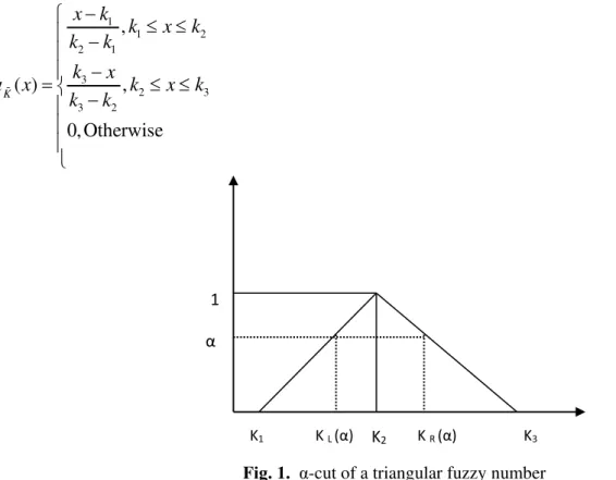
Definition 2.3 A fuzzy number K~ =( ,k k k_{1 2}, ₃) where k1 < k2 <k3 and defined onR, is called a triangular

1

1 2

2 1

3

2 3

3 2

,

( ) ,

0, Otherwise K

x k

k x k

k k

k x

x k x k

k k

µ

−

 _{≤ ≤}

 − 

− 

=_{ −} ≤ ≤

   



Fig. 1. α-cut of a triangular fuzzy number When k₁ =k₂ =k₃ =k , we have fuzzy point( , , )k k k =k.

The family of all triangular fuzzy numbers on Ris denoted as

(

)

{

1, 2, 3 1 2, 3 1, 2, 3

}

N

F = k k k k <k <k ∀k k k ∈R

The

α

-cut of ~

1 2 3

( , , ) N, 0 1,

K = k k k ∈F ≤ ≤α isK( )α = _K_L

( )

α ,K_R

( )

α _,

where K_L( )α = +k₁ (k₂−k₁)α and K_R( )α = −k₃ (k₃−k₂)α are the left and right endpoints ofK( )α .

Definition 2.4 If K~ =( ,k k k_{1 2}, ₃) is a triangular fuzzy number then the signed distance form Kto 0 is defined as

[

]

1

~ ~

0

( 0) _L( ) , _R( ) , 0 d K = d_ k α _α K α _α _

 

∫

 =1

(

₁ 2 _{2 3}

)

4 k + k +k

3.Assumptions and Notations

The following notations and assumptions have been used in developing the model.

3.1 Notations

I(t) : instantaneous inventory level at time t

Q : order level

D(p) = D = a - bp : price dependent demand

( )

D p =D = −a bp : fuzzy price dependent demand

A : replenishment cost (ordering cost) for replenishing the items c : unit purchase cost of retailer

h : holding cost per unit per unit time excluding interest charge

θ : deterioration rate and 0≤ <θ 1

μ(μ > 1) : mark up rate 1

α

1

p = μc : selling price per unit

M : credit period offered by the supplier Ie : interest earned by the retailer ($ per year)

Ip : interest payable to the supplier ($ per year)

td : time period during which no deterioration occurs.

T : replenishment cycle length Bi : breakeven point, i=1, 2, 3

AP(.)(μ, T) : total profit in case (.)

AP (.) : total profit in combine form for all cases APd (.) : total profit after defuzzify

3.2 Assumptions

(i) Replenishment rate is infinite and lead time is negligible.

(ii) The inventory planning horizon is infinite and the inventory system involves only single commodity and single stocking point.

(iii) The entire lot size is delivered in one batch. (iv) Shortages are not allowed.

(v) Demand rate is assumed to be a function of selling price i.e. D p

( )

= −a bpwhich is a function of selling price (p), where a, b are positive constants and 0 < b < a / p. Further, a & b are assumed as triangular fuzzy number.

4. Model Formulation

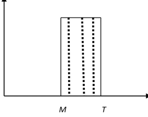
This is an EOQ model for a single non-instantaneous deteriorating item with permissible delay in payments. Initially, a lot size of Q units enters the inventory system and depletes due to demand in the interval[0, ]td . After that i.e. in the time interval [ , ]t Td this is deplete due to the combine effect demand and deterioration. Att =T, the inventory stock is exhausted. At any time t the inventory level can be shown by following differential equation.

Fig. 2. Inventory level at any time

( )

,

dI t D

dt = 0≤t ≤td (1)

( )

_{( )}

,

dI t

I t D

dt +θ = − td < ≤t T (2)

0 td _T

Q

These differential equations solve with using boundary conditions I( 0 ) = Q, and I( T ) = 0 respective are as follows:

( )

,

I t = −Q Dt 0≤t ≤td (3)

( )

D

(

(T t) _{1 ,}

)

I t eθ

θ

−

= − td < ≤t T (4)

For continuity of I t

( )

att=t_d,it follows from Eq. (3) and Eq. (4) that

( )

(

T td 1

)

d

D

Q Dt eθ

θ −

− = −

This implies that the maximum inventory level per cycle is

( )

(

)

1

1 ,

d

T t d

Q D t eθ

θ −

 

= _ + − _

  (5)

The number of deteriorated unit Q−DTis

( )

(

)

1

1

d

T t d

D t T eθ

θ

−

 

= _ − + − _

  (6) Now, the profit function per unit time can be expressed as

(

)

1

,

AP T

T

µ = [<Total selling revenue > + <Interest earned > - < Total purchase cost > -

<Ordering Cost> - <Holding Cost> - <Interest paid >] where

a) Ordering cost per cycle = A

b) The inventory holding cost per cycle

( )

( )

0

d

d

t T

t

h I t dt I t dt

= _ + _



∫

∫



(

)

(

)

2

( )

2 1 1 ( )

2

d

T t d

d d

Dt D

h eθ θt T t

θ

−

 

= _ + − + − − _

  (7) c) The purchase cost per cycle = cQ

( )

(

)

1

1

d

T t d

cD t eθ

θ −

 

= _ + − _

 

(8)

d) The Sales Revenue per cycle =DTp (9)

For the calculation of interest earned and payable, two possible cases depending on the values of interest earned and payable rate i.e. I_e<I_p and I_e≥I_p arises.These two cases have been discussed in following two sections.

Section 1: I_e<I_p

In this section, the interest earned rate (I_e), is assumed to be less than the interest payable rate (I_p). Further, depending upon values of M, td and T there can be three possible cases:

Case 1.1:0<M ≤ <td T, Case 1.2: 0< <td M ≤T and Case 1.3: 0< < <td T M

Case 1.1: 0<M ≤ <t_d T

In this case, the retailer tries to pay off the total purchase cost to the supplier as soon as possible. Therefore, up to time period M, the total sales revenue generated by the retailer is DMp and he also earns

interest on this sales revenue which is1 2

Hence, the total amount available at time M is sum of sales revenue and interest earned on regular sales revenue i.e.

2

1

(say)

2 e

DMp+ DM pI ≡W (10)

At this point of time, retailer wishes to settle his account with the supplier. Which gives birth to another two sub-cases viz. W <Qc _andW ≥Qc.

Sub case 1.1.1: W <Qc

Here, the retailer’s sales proceeds (W) is less than the amount payable (Qc) to the supplier. In this situation, supplier may either agree to receive the partial payment or not. Thus, further two scenarios generated i.e. when partial payment is acceptable at M _{and the rest amount is to be paid any time after M} and when partial payment is not acceptable at M but the full payment is acceptable by the supplier any time after M.

Scenario 1.1.1.1: When partial payment is acceptable at M and the rest amount is to be paid any time

after M. This scenario is further divided into two situations i.e.

(a)When the rest amount continuously is paid after M and

(b)When the rest amount is paid as a single installment any time after M.

Scenario1.1.1.1 (a): When the rest amount is paid continuously up to breakeven pointB₁ (say) after M

In this scenario, the retailer pays Wamount at M and the rest amount

(

cQ W−

)

along with the interest

charged will be paid continuously from M to some payoff timeB₁ (says).

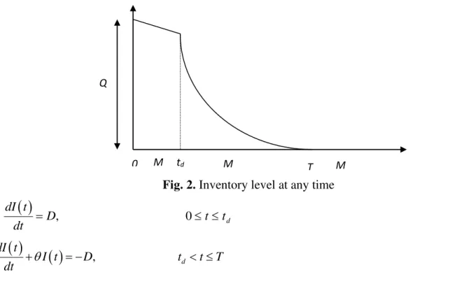
Fig. 3. Interest earned in scenario 1.1.1.1. (a) Fig. 4. Interest payable in scenario 1.1.1.1. (a) The interest payable during the period

[

M B, ₁

]

= 1

(

)(

₁

)

2 cQ W− B −M Ip and

The total amount payable during

[

M B, ₁

]

=

(

)

1

(

)(

₁

)

2 p

cQ W− + cQ W− B −M I

⇒ Att=B₁, the total amount payable to the supplier = the total amount available to the retailer

⇒

(

)

1

(

)(

₁

)

(

₁

)

2 p

cQ W− + cQ W− B −M I =D B −M p

(

)

(

)

1

2

2 p

cQ W

B M

Dp cQ W I

−

⇒ = +

− − (11)

Now, from time (B1) onwards the retailer starts accumulating profit from the sales and earns interest

during the period

[

B T₁,

]

The total sales revenue = D T

(

−B p₁

)

and

Interest earned =1

(

₁

)

2

2D T −B pIe.

Therefore, the total profit per unit time for this case is given by

(

)

1.1.1.1.( )

1 ,

a

AP T

T

µ = [<Total selling revenue during

[

B T₁,

]

> + <Interest earned during

[

B T₁,

]

> -

<Ordering Cost> - <Holding Cost>]

( )

(

)

(

)

2 2

(

_{( )}

)

(

)

1.1.1.1.( ) 1 1 2

1 1

, 1 1 ( )

2 2

d

T t d

a e d d

Dt D

AP T D T B p D T B pI A h e t T t

T

θ

µ θ

θ

−

  

= _ − + − − − _ + − + − − _

 

  (12)

Where

(

)

(

)

1

2

2 _p

cQ W

B M

Dp cQ W I

−

= +

− − (13)

Scenario 1.1.1.1(b): When the rest amount is paid at a breakeven point B₂ (say) after M

In this scenario, supplier accepts the payment only on two installments first is at time M and second is at some payoff time B₂(says). The retailer pays amount W at M and the rest amount

(

cQ W−

)

along with

the interest chargedwill be paid ata breakeven pointB₂. Now, at timet=B₂, retailer would generate an amount of D B( ₂−M p) from sales revenue for the period

[

M B, ₂

]

and also earn interest from the continuous interest earn on the selling revenue generated during the same.

Fig. 5. Interest earned in scenario 1.1.1.1. (b) Fig. 6. Interest payable in scenario 1.1.1.1. (b) The interest payable during the period

[

M B, ₂

]

=

(

cQ W−

)(

B₂−M I

)

_p

The interest earned during the period

[

M B, ₂

]

= 1 ( ₂ )2 2D B −M pIe

The total amount payable atB₂ =

(

cQ W−

) (

+ cQ W−

)(

B₂−M I

)

_pand

The total amount earn during the period

[

M B, ₂

]

= D B M p D B M pIe 2 2

2 ( )

2 1 )

( − + −

⇒ Att=B₂, the total amount payable to the supplier = the total amount available to the retailer

⇒

(

) (

)(

)

(

)

(

)

2

2 2 2

1 2

p e

cQ W− + cQ W− B −M I =D B −M p+ D B −M pI

(

)

(

)

1

2 ₂

2

1

2

e p p p e e

e

B Dp DpI M QcI I W Dp QcI WI DpQcI

DpI

 

 

⇒ = _− + + − + − + + _

 

  (14)

Now, from this point onwards the retailer starts generating profit from the sales and also earns interest on the same i.e. during the period

[

B T₂,

]

The total sales revenue = D T

(

−B₂

)

p and Interest earned =1

(

₂

)

2

2D T −B pIe.

Therefore, the total profit per unit time for this case is given by

(

)

1.1.1.1.( )

1 ,

b

AP T

T

µ = [<Total selling revenue during

[

B T₂,

]

> + <Interest earned during

[

B T₂,

]

> -

<Ordering Cost>-<Holding Cost>]

( )

(

)

(

)

2 2

(

( )

)

(

)

1.1.1.1.( ) 2 2 2

1 1

, 1 1 ( )

2 2

d

T t d

b e d d

Dt D

AP T D T B p D T B pI A h e t T t

T

θ

µ θ

θ

−

  

= _ − + − − − _ + − + − − _

 

  (15)

Where

(

(

)

)

1

2 ₂

2

1

2

e p p p e e

e

B Dp DpI M QcI I W Dp QcI WI DpQcI

DpI

 

 

= _− + + − + − + + _

 

 

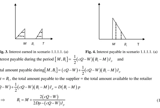
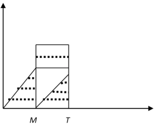
Scenario 1.1.1.2: When full payment is to be made at the breakeven point B₃(say) after M

In this scenario, Supplier wants the full payment at some fixed point B₃ (says) after M when it is possible. Now, at timet=M , the retailer has Wamount and he will earn the interest on this amount for the period

[

M B, 3

]

, but he has to pay the interest for the time period

[

M B, 3

]

. Further, at timet=B3, retailer would generate an amount of D B( ₃−M p) from sales revenue for the period

[

M B, ₃

]

and also earn interest from the continuous interest earn on the selling revenue generated during the same.

Fig. 7. Interest earned in scenario 1.1.1.2 Fig. 8. Interest payable in scenario 1.1.1.2 The interest earned on accumulated amountWfor the time period

[

M B, ₃

]

= WI_e

(

B₃−M

)

The interest earned on the continuous sales revenue from time period

[

M B, ₃

]

=1

(

₃

)

2

2D B −M pIe.

Hence, the total interest earned during the time period

[

M B, 3

]

=

(

)

(

)

2

3 3

1 2

e e

WI B −M + D B −M pI

The total amount available to the retailer at

M T

(

)

(

)

(

)

2

3 3 3 3

1 2

e e

B =W +D B −M p WI+ B −M + D B −M pI

The interest payable during the period

[

M B, ₃

]

=QcI_p

(

B₃−M

)

and

The total amount payable at B₃= Qc QcI+ _p

(

B₃−M

)

⇒ Att=B₃, the total amount payable to the supplier = the total amount available to the retailer

(

)

(

)

(

)

(

)

2

3 3 3 3

1 2

p e e

Qc Qc B+ −M I =W+D B −M p WI+ B −M + D B −M pI

(

)

(

)

1

2 ₂

3 1

) 2

e p e e p e

e

B Dp DpI M QcI I W WI QcI Dp DpQcI

DpI

 

 

⇒ = _− + + − + − + + _

 

 

₍₁₆₎

Now, from this point onwards the retailer starts generating profit from the sales and also earns interest on the same i.e. during the period

[

B T₃,

]

The total sales revenue during the time period

[

B T₃,

]

= D T

(

−B₃

)

pand

The interest earned during same period =1

(

₃

)

2

2D T −B pIe.

Therefore, the total profit per unit time for this case is given by

(

)

1.1.1.2

1 ,

AP T

T

µ = [<Total sales revenue during

[

B T₃,

]

> + <Interest earned during

[

B T₃,

]

> -

<Ordering Cost> - <Holding Cost>]

( )

(

)

(

)

2 2

(

( )

)

(

)

1.1.1.2 3 3 2

1 1

, 1 1 ( )

2 2

d

T t d

e d d

Dt D

AP T D T B p D T B pI A h e t T t

T

θ

µ θ

θ

−

  

= _ − + − − − _ + − + − − _

 

  (17)

(

)

(

)

1

2 ₂

3 1

Where )e p e e p 2 e

e

B Dp DpI M QcI I W WI QcI Dp DpQcI

DpI

 

 

= _− + + − + − + + _

 

 

Sub case 1.1.2: W ≥Qc

In this sub case, retailer has to pay only Qcamount to the supplier at time M,he will earn the interest on the excess amount

(

W−Qc

)

for the time period

[

M,T

]

. Further, after timet=M , the retailer continuously sales the products and uses the revenue to earn interest.

Fig. 9. Interest earned in sub case 1.1.2

The interest earned on the excess amount

(

W −Qc

)

for the period

[

M,T

]

=

(

W −Qc T

)

( −M I) _e

The interest earned on the sales revenue during the period

[

M,T

]

= D

(

T M

)

2pI_e

2

1 ₋

Therefore, the total profit per unit time for this case is given by

1.1.2

1 ( , )

AP T

T

µ = [< Total sales revenue during

[

M,T

]

> + <Interest earned on the sales revenue

during

[

M,T

]

> + <Remaining excess amount after paying the amount to the supplier > + <Interest earned on the excess amount during

[

M,T

]

> - <Ordering Cost> - <Holding Cost>]

(

)

(

)

(

) (

{

)

}

2

(

( )

)

(

)

1.1.2 2

1 1

( , ) 1 1 1 1 ( )

2 2

d

T t d

e e d d

Dt D

AP T D T M p T M I W Qc T M I A h e t T t

T

θ

µ θ

θ

−

    

= _ − _ + − _+ − + − − − _ + − + − − _

  _{ }

  (18)

Case 1.2: 0< <t_d M ≤T

In this case, permissible delay period M lies between the time t_d at which deterioration start and replenishment cycle timeT. In this case the mathematical formulation is same as of Case 1.1 i.e.

0<M ≤ <t_d T. So the mathematically formulation for this case is not necessitate.

Case 1.3: 0< < <t_d T M

In this case, permissible delay period M is greater than the replenishment cycle timeT . The retailer will pay off the total amount owed to the supplier at the end of the trade credit periodM. Therefore, there is no interest payable to the supplier but the retailer uses the sales revenue to earn interest at the rate of I_e

during the period

[

0,M

]

.

Fig. 10. Interest earned in case 1.3

The interest earned during the period

[ ]

0,T = DT2pI_e

2 1

and

The interest earned during the period

[

T,M

]

=DTp TI_eI_e

(

M −T

)

  

  +

2 1 1

Therefore, the total profit per unit time for this case is given by

1.3

1 ( , )

AP T

T

µ = [<Total sales revenue during [0, T]> + <Interest earned on sales revenue during

[0, M] > - <Purchasing cost> - <Ordering cost> - <Holding cost>]

(

)

2

(

)

2

(

( )

)

(

)

1.3 2

1 1 1

( , ) 1 1 1 ( )

2 2 2

d

T t d

e e d d

Dt D

AP T DTp Qc DT p DTp TI I M T A h e t T t

T

θ

µ θ

θ

−

 _{ }  

= _ − + + _ + _ − − − _ + − + − − _

  _{ }

  (19)

Section 2: I_e ≥I_p

Here, the interest earnedI_e, is taken to be greater than and equal to the interest chargesI_p. Further, depending upon values of M, td and T there may arise three possible cases as follows:

Case 2.1: 0<M ≤ <t_d Tand Case 2.2: 0< <t_d M ≤T Case 2.3: 0< < <t_d T M

Case 2.1: 0<M ≤ <t_d T

In this scenario, retailer would make the payment at T not at M. SinceIe ≥Ip, the retailer never pays any amount to the supplier before the end of cycle (T).

Fig. 11. Interest earned in case 2.1 Fig. 12. Interest payable in case 2.1 The total interest payable in one cycle = Qc T

(

−M I

)

_p and

The total interest earned in one cycle after M =

(

)

1

(

)

2

2

e e

WI T−M + D T−M pI

Hence, the total amount payable by the retailer at T = Qc(1+

(

T −M I

)

_p) Therefore, the total profit for the cycle for this case is given by

2.1

1 ( , )

AP T

T

µ = [< Total selling revenue during

[ ]

0,T > + <Interest earned on the sales revenue

during

[ ]

0,T > - < total amount paid as well as interest payable at T> - <Ordering Cost> - <Holding Cost>]

( ) 2 ( ) ( )2 ( ) 2

(

( )

)

( )

2.1 2

1 1 1

( , ) 1 1 ( )

2 2 2

d

T t d

e e e p d d

Dt D

AP T DTp Qc DM pI WI T M Dp T M I Qc T M I A h e t T t

T

θ

µ θ

θ

−

  

=  − + + − + − − − − −  + − + − − 

  

  (20)

Case 2.2: 0< <t_d M ≤T

In this case, the mathematical expression of total profit per unit time AP_2.2( , )µ T is same as of in case (2.1).

Case 2.3: 0< < <t_d T M

The mathematical expression of total profit per unit time AP_2.3( , )µ T is also same as of in case (1.3). Hence, the total profit per unit time AP( , )µ T for the inventory system can be expressed as

p 1.1.1.1.( ) 1.1.1.1.( ) 1.1.1.2 1.1.2 1.2.1.1.( ) 1.2.1.1.( ) 1.2.1.2 1.2.2 1.3 2.1 2.2 2.3

if 0<M , W<cQ, <I , parti ( , ) ( , ) ( , ) ( , ) ( , ) ( , ) ( , ) ( , ) ( , ) ( , ) ( , ) ( , ) ( , ) d e a b a b

t T I

AP T AP T AP T AP T AP T AP T AP T AP T AP T AP T AP T AP T AP T µ µ µ µ µ µ µ µ µ µ µ µ µ ≤ < = p p p

allly and rest amount paid continuosly if 0<M , W<cQ, <I , partiallly and rest amount second shippment if 0<M , W<cQ, <I , and full amount made after t = M if 0<M , W cQ and <I

d e

d e

d e

t T I

t T I

t T I

≤ < ≤ < ≤ < ≥

p

p

p

if 0< , W<cDT, <I , partiallly and rest amount paid continuosly if 0< , W<cDT, <I , partiallly and rest amount second shippment if 0< , W<cDT, <I , and full amount made after t = M

if 0< , W

d e

d e

d e

d

t M T I

t M T I

t M T I

t M T < ≤ < ≤ < ≤

< ≤ _p

p

p

p

p

cDT and <I if 0< and <I

if 0<M , I

if 0< , I

if 0< , I

e d e d e d e d e I

t T M I

t T I

t M T I

t T M I             ≥  < ≤ 

 _{≤ < ≥}



 _{< ≤ ≥}



< ≤ ≥ 

(21)

For the convenience, we let the twelve events as

1 { |0<M d , W<cQ, <I , partiallly and rest amount paid continuosly}e p

E = T ≤ <t T I

(22)

2 { | 0<M d , W<cQ, <I , partiallly and rest amount second shippment}e p

E = T ≤ <t T I (23)

3 { | 0<M d , W<cQ, <I , and full amount made after t = M}e p

E = T ≤ <t T I (24)

4 { | 0<M d , W cQ, <I , and full amount made at t = M}e p

E = T ≤ <t T ≥ I (25)

5 { |0< d M , W<cQ, <I , partiallly and rest amount paid continuosly}e p

E = T t < ≤T I (26)

6 { | 0<d M , W<cQ, <I , partiallly and rest amount second shippment}e p

E = T t < ≤T I (27)

7 { | 0<d M , W<cQ, <I , and full amount made after t = M}e p

E = T t < ≤T I (28)

8 { | 0<d M , W cQ, <I , and full amount made at t = M}e p

E = T t < ≤T ≥ I (29)

9 { | 0< d and e<I }p

E = T t < ≤T M I (30)

10 { | 0<M d and e I }p

E = T ≤ <t T I ≥ (31)

11 { | if 0<d and e I }p

E = T t <M ≤T I ≥ (32)

12 { | 0<d and e I }p

E = T t < ≤T M I ≥ (33)

and define the characteristic functions as

1 ( ) 0 j c j j T E t T E

φ _{= } ∈

∈

 j =1 ... 12, (34)

and also let

(

)

(

)

(

( )

)

2

( )

1 2

1 1

1 1 ( ) 1

2

d

d T t

T t d

d d d

Dt D

H A h e t T t cD t T e

T θ θ _θ θ θ − −      = _ + _ + − + − − _+ _ − + − _    

  (35)

1 ( ), 1, ...,12

k k k

H ₊ = X φ t k= ₍₃₆₎

where

1 1.1.1.1.( ) 1 2 1.1.1.1.( ) 1 3 1.1.1.2 1 4 1.1.2 1

5 1.2.1.1.( ) 1 6 1.2.1.1.( ) 1 7 1.2.1.2 1 8 1.2.2 1

9 1.3 1 10

( , ) , ( , ) , ( , ) , ( , ) ,

( , ) , ( , ) , ( , ) , ( , ) ,

( , ) ,

a b

a b

X AP T H X AP T H X AP T H X AP T H

X AP T H X AP T H X AP T H X AP T H

X AP T H X

µ µ µ µ

µ µ µ µ

µ

= − = − = − = −

= − = − = − = −

= − =AP2.1( , )µT −H X1, 11=AP2.2( , )µT −H X1, 12= AP2.3( , )µT −H1,

The Profit function in Eq. (29) can be reduced to collective form with the help of Eq. (30) to Eq. (45), as follows:

12

1 1

1

( , ) _k

k

AP µ T H + H

=

 

=_{ }−



∑

 (38)

5. Fuzzy Model

Due to fuzziness, the decision maker unable to determine the exact value of the parameters in business environments, therefore the approximate values of the parameters are considered. In this model, deteriorating rate θ θ=  and demand rate D=D are considered in fuzzy environment. By substituting

θ θ= and D=D = −a bp in Eq. (38), the crisp model would convert into fuzzy model as

 12

1 1

1

( , ) _k

k

AP µ T H ₊ H

=

 

=_{ }−



∑

   (39)

As demand function is taken to be triangular fuzzy number, therefore AP( , )µ T is also triangular fuzzy number as



₍

₎

1 2 3

( , ) , ,

AP µ T = AP AP AP (40)

where

4 12

( 1) 1

1

, 1, 2,3

i i

i k

k

AP H ₊ H ₋ i

=

 

=_{ }− =



∑

 (41)

1 2 3

( , , ) and 1,...,13

k k k k

H = H H H k = (42)

( )

(

)

2

(

( )

)

(

)

1 2

4 4

1 1

1 1 1 ( )

2

j d j d

j

T t j d j T t

j d j d d

j j

D t D

H A cD t T e h e t T t

T

θ θ _θ

θ θ − − − −    _ _   = _ + _ − + − _+  + − + − − _      

  (43)

(

4

)

(

4

)

2

2 1 1 1

1 1

( ) 2

j j j j j e

H D T B p D T B pI t

T − − φ

 

= _ − + − _

  (44)

(

4

)

(

4

)

2

3 2 2 2

1 1

( ) 2

j j j j j e

H D T B p D T B pI t

T − − φ

 

= _ − + − _

  (45)

(

4

)

(

4

)

2

4 3 3 3

1 1

( ) 2

j j j j j e

H D T B p D T B pI t

T − − φ

 

= _ − + − _

  (46)

(

)

(

)

(

)

{

(

)

}

5 4 4

1 1

1 1 ( )

2

j j e j j e

H D T M p T M I W Q c T M I t

T − φ

   

= _ − _ + − _+ − + − _

 

  (47)

(

4

)

(

4

)

2

6 1 1 5

1 1

( ) 2

j j j j j e

H D T B p D T B pI t

T − − φ

 

= _ − + − _

  (48)

(

4

)

(

4

)

2

7 2 2 6

1 1

( ) 2

j j j j j e

H D T B p D T B pI t

T − − φ

 

= _ − + − _

  (49)

(

4

)

(

4

)

2

8 3 3 7

1 1

( ) 2

j j j j j e

H D T B p D T B pI t

T − − φ

 

= _ − + − _

  (50)

(

)

(

)

(

)

{

(

)

}

9 4 8

1 1

1 1 ( )

2

j j e j j e

H D T M p T M I W Q c T M I t

T − φ

   

= _ − _ + − _+ − + − _

 

(

)

2

(

)

10 4 9

1 1 1

1 ( )

2 2

j j j j j e e

H D Tp Q c D T p D Tp TI I M T t

T − φ

   

= _ − + + _ + _ − _

 

  (52)

(

)

₂

(

)

(

)

2

(

)

11 4 4 10

1 1 1

( )

2 2

j j j j e j e j e j p

H D Tp Q c D M pI W I T M D p T M I Q c T M I t

T − − φ

 

= _ − + + − + − − − _

  (53)

(

)

2

(

)

(

)

2

(

)

12 4 4 11

1 1 1

( )

2 2

j j j j e j e j e j p

H D Tp Q c D M pI W I T M D p T M I Q c T M I t

T − − φ

 

= _ − + + − + − − − _

  (54)

(

)

2

(

)

13 4 12

1 1 1

1 ( )

2 2

j j j j j e e

H D Tp Q c D T p D Tp TI I M T t

T − φ

   

= _ − + + _ + _ − _

 

  (55)

2

1 2

j j j e

W =D Mp+ D M pI (56)

( )

(

)

4 1

1

j T td

j j d j

Q D t eθ

θ

−

−

 

= _ + − _

  (57)

(

)

(

4

)

1 4 4 2 2 j j j

j j j p

cQ W

B M

D p cQ W I

−

− −

−

= +

− − (58)

(

)

(

)

1

2 ₂

2 4 4 4

4

1

2

j j j e j p p j j j p j e j j e

j e

B D p D pI M Q cI I W D p Q cI W I D pQ cI

D₋ pI − − −

 

 

= _− + + − + − + + _

 

  (59)

(

)

(

)

1

2 ₂

3 4 4 4 4

4 1

2

j j j e j p e j j e j p j j j e

j e

B D p D pI M Q cI I W W I Q cI D p D pQ cI

D₋ pI − − − −

 

 

= _− + + − + − + + _

 

  (60)

(4 ) and

j j j

D =a −pb ₋ p=µc ₍₆₁₎

Now defuzzify the fuzzy profit function by, using the signed distance method, measured from AP to 0

[

1 2 3

]

1

( , ) 2

4

d

AP T µ = AP+ AP +AP (62)

6. Solution Procedure

To determine the optimal values of µ and T, differentiate partially the profit function, AP_d( , )µ T with respect to µ and T and equating to zero, we obtain:

( , ) 0

d

AP µ T

µ

∂ ₌

∂ (63)

and APd( , )T 0

T

µ

∂ ₌

∂ (64)

2

2 ( , )

0 d

AP µ T µ

∂ _<

∂ and

2 2 ( , ) 0 d AP T T µ ∂ <

∂ (65)

2 2 2 2

2 2

( , ) ( , ) ( , ) ( , )

0

d d d d

AP T AP T AP T AP T

T T T

µ µ µ µ

µ µ µ

∂ ∂ ₋∂ ∂ _>

∂ ∂ ∂ ∂ ∂ ∂ (66)

The profit functions of the present problem under various cases are highly non-linear and too complicated to solve. Further also it is not easy to show their concavity mathematically, alternatively, we have shown the concavity of these profit functions graphically for all the cases and sub cases with the help of computer software MATLAB. Similarly, the optimal values of various decision variables i.e. mark up rate and cycle length is determined with the help of MS- Excel’s solver which uses the GRG2 algorithm.

Fig. 13. Optimal Total Profit versus T and μ Fig. 14. Optimal Total Profit versus T and μ

7. Special Case:

 If we assumea₁ =a₂ =a₃ =a b, ₁=b₂ =b₃ =bandθ θ₁= ₂ =θ₃ =θ and substitute in Eq. (62), then

( , )

d

AP µ T becomes the crisp total profit function i.e.

12 1 1 1 ( , ) ( , ) d k k

AP T µ H ₊ H AP T µ

=

 

=_{ }− =



∑

 (67)

That is, the fuzzy case becomes the crisp case.

 When td = 0 (deterioration is instantaneous)

Then, the total profit per unit time reduced to

p 1.2.1.1.( ) p 1.2.1.1.( ) 1.2.1.2 1.2.2 1.3 2.2 2.3

if 0<M , W<cDT, <I , partiallly and rest amount paid continuosly ( , )

if 0<M , W<cDT, <I , partiallly and ( , ) ( , ) ( , ) ( , ) ( , ) ( , ) ( , ) e a e b T I AP T T I AP T AP T

AP T AP T

AP T AP T AP T µ µ µ µ µ µ µ µ ≤ ≤ = p p p p p

rest amount second shippment if 0<M , W<cDT, <I , and full amount made after t = M

if 0<M , W cDT and <I if 0<T and <I if 0< and I if 0< and I

e e e e e T I T I M I

M T I

M T I

    _≤  _{≤ ≥}   _≤  ≤ ≥   _{≤ ≥}  (68)

8. Algorithm

The procedure for determining the optimal values of decision variables are as follows:

For Ie<Ip

Step 1: For event E1, determineµ*, and T* from Eq. (63) and Eq. (64). If µ* and T* are in E1 then

calculate APd (µ*, T*) from (62), this gives AP(d) 1.1.1.1.(a) (µ*, T*). Otherwise go to step 2.

Step 2: For event E2, determineµ* and T* from Eq. (63) and Eq. (64). If µ* and T*are in E2 then calculate

APd (µ*, T*) from (62), this gives AP (d) 1.1.1.1. (b) (µ*, T*). Otherwise go to step 3.

Step 3: For event E3, determineµ*and T* from Eq. (63) and Eq. (64). If µ* and T*are in E3 then calculate

APd (µ*, T*) from (62), this gives AP (d) 1.1.1.2 (µ*, T*). Otherwise go to step 4.

Step 4: For event E1, determineµ*, and T* from Eq. (63) and Eq. (64). If µ* and T* are in E1 then

calculate APd (µ*, T*) from (62), this gives AP (d) 1.1.2 (µ*, T*).Otherwise go to step 5.

Step 5:

For event E5, determineµ

*_{, and T}* _{from Eq. (63) and Eq. (64). If} µ* _{and T}* _{are in E} 5 then

calculate APd (µ*, T*) from (62), this gives AP (d) 1.2.1.1. (a) (µ*, T*). Otherwise go to step 6.

Step 6: For event E6, determineµ* and T* from Eq. (63) and Eq. (64). If µ* and T*are in E6 then calculate

APd (µ*, T*) from (62), this gives AP (d) 1.2.1.1. (b) (µ*, T*). Otherwise go to step 7.

Step 7: For event E7, determineµ*and T* from Eq. (63) and Eq. (64). If µ* and T*are in E7 then calculate

APd (µ*, T*) from (62), this gives AP (d) 1.2.1.2 (µ*, T*). Otherwise go to step 8.

Step 8: For event E8, determineµ*, and T* from Eq. (63) and Eq. (64). If µ* and T* are in E8 then

calculate APd (µ*, T*) from (62), this gives AP (d) 1.2.2 (µ*, T*).Otherwise go to step 9.

Step 9: For event E9, determineµ* and T* from Eq. (63) and Eq. (64). If µ* and T*are in E9

then calculate APd (µ*, T*) from (62), this gives AP (d) 1.3 (µ*, T*). Otherwise go to step

10.

For I_e≥I_p

Step 10: For event E10, determineµ*and T* from Eq. (63) and Eq. (64). If µ* and T* are in E10 then

calculate APd (µ*, T*) from (62), this gives AP(d)2.1 (µ*, T*). Otherwise go to step 11.

Step 11: For event E11, determineµ*, and T* from Eq. (63) and Eq. (64). If µ* and T*are in E11 then

calculate APd (µ*, T*) from (62), this gives AP (d) 2.2 (µ*, T*).Otherwise go to step 12.

Step 12: For event E12, determineµ*, and T* from Eq. (63) and Eq. (64). If µ* andT*are in E12

then calculate APd (µ*, T*) from (62), this gives AP (d) 2.3 (µ*, T*).Otherwise go to

step1.

The optimal solution of the inventory system can be found by comparing the total profits of all the cases. Hence the optimal total profit of the system is given by

APd (µ*, T*) = max [APd (1) (µ*, T*), APd (2) (µ*, T*)]

9. Numerical Examples

Table 1

Values of parameters of different examples

Example A (in$)

h

(in $) θ td c

Ie

(per $)

Ip

(per $)

M

(days)

1. Ie < Ip 150 10 (0.08, 0.1, 0.14) (145,150,155) (0.06, 0.07, 0.08) 0.2 100 0.12 0.15 30/365

=0.082

2. Ie≥ Ip 150 10 (0.08, 0.1, 0.14) (145,150,155) (0.06, 0.07 ,0.08) 0.2 100 0.2 0.15 30/365

=0.082

Table 2

Result of Example 1 and 2 for different cases, sub cases and scenarios

Section Case

Sub-case Scenarios μ T B Wi p = μc Q Profit Remark

Ie < Ip

1.1 1.1.1

1.1.1.1.a 1.50 1.23 0.57 2481.06 150 45 1334.52

Scenario1.1.1.1.b 1.1.1.1.b 1.48 1.02 0.47 2237.85 148 37 1381.43

1.1.1.2 1.41 0.97 0.51 2153.74 141 31 1276.09

1.1.2 - 1.43 0.94 - 2075.34 143 20 1235.87

1.2 1.2.1

1.2.1.1.a 1.47 0.86 0.54 2562.61 147 35 1237.65 1.2.1.1.b 1.42 0.73 0.45 2407.25 142 26 1187.65 1.2.1.2 1.38 0.53 0.42 2217.53 138 23 948.35

1.2.2 - 1.41 0.76 - 2147.07 141 21 1176.54

1.3 1.49 M - - 149 25 1043.47

Ie≥ Ip

2.1 - - 1.58 1.07 0.73 3547.34 158 42 1457.73

Scenario 2.1

2.2 - - 1.52 0.65 - 2467.07 152 34 1345.67

2.3 - - 1.48 M - - 148 27 1136.27

Using the proposed algorithm the results are as follows:

For I_e<I_p

* 1

µ =1.48, p₁* =$148, B₁*=0.47 year, T₁*= 1.02 year, Q₁*= 37 units and total profit = $1381.43 (Scenario 1.1.1.1.b)

For Ie≥Ip *

2

µ =1.58, * 2

p =$158, * 2

B = 0.73 year, * 2

T = 1.07 year, * 2

Q = 42 units and total profit = $1457.73 (Case 2.1)

10. Sensitivity Analysis

To study the effects of changes of different parameters [like, A (ordering cost), a, b (location parameter of demand), h (holding cost), c (unit purchase cost of retailer), M (Permissible delay in payment) on the optimal policies, sensitivity analyses have been performed numerically. These analyses have been carried out by changing -20% to +20% for one parameter keeping other parameters as same. The results of these analyses have been displayed in Table 3.

From Table 3, the following inferences can be made:

 One can easily observe that with the increase in value of ordering cost (A), the optimal cycle length (T), optimal order quantity (Q) increases; but the total profit (AP) decreases.

 With the increase in the holding cost (h), the total profit (AP) decreases as there is an increase in carrying cost.

 With the increase in the value of (a), the total profit (AP) increases whereas as the value of (b) increases, the total profit (AP) decreases.

 As the cost per unit (c) increases, there is a decrement in the value of total profit (AP). This reveals the natural trend of cost-profit analysis.

 It is clearly observe that as the credit period (M) increases, both optimal order quantity (Q) and total profit (AP) increases.

 It is observed from table 3, as the deterioration rate (θ) increases then there is significant decrease in total profit (AP) & increase in order quantity (Q) because a rise in deterioration rate (θ) causes an increase in the cost of deteriorated units, which ultimately increase the total cost.

 From the table 3 it is clearly visible that with an increase in the value of td, it can be observed that

cycle length (T), order quantity (Q) and total profit (AP) increases. This clearly indicates the positive impact of non-instantaneous deteriorating items in the inventory modelling. As the period for non-deterioration (td) increases, the deterioration cost for items decreases which accounts for

larger profits for the company.

Table 3

Effect of changes in the system parameters

Parameters % changes T B Q Profit

A

-20% -1.03 -21.39 -28.32 -26.64 4.56

-10% -0.48 -12.03 -15.54 -14.73 1.43

10% 0.75 19.58 18.59 18.23 -0.86

20% 1.53 38.84 37.15 35.31 -2.36

a

-20% -13.23 28.64 47.65 -35.08 -75.34

-10% -6.17 11.75 23.05 -15.69 -42.81

10% 6.13 -9.23 -15.86 15.02 49.83

20% 12.56 -12.45 -24.63 29.65 93.78

b

-20% 4.04 58.53 15.07 53.91 17.89

-10% 3.09 34.04 -23.09 32.76 13.57

10% -3.18 -34.98 -33.11 -33.05 -13.90

20% -3.92 -57.31 9.87 -50.61 -17.07

h

-20% -0.19 7.24 7.72 7.36 4.72

-10% -0.08 3.34 3.56 3.43 1.83

10% 0.51 -2.76 -3.18 -3.69 -1.75

20% 0.85 -6.43 -5.83 -6.87 -4.21

c

-20% 15.37 5.63 -29.63 34.27 56.43

-10% 7.42 2.27 -13.54 15.53 30.25

10% -5.83 -2.84 13.82 -14.67 -35.04

20% -12.75 -5.82 28.32 -37.92 -73.25

M

-20% 0.02 1.33 0.99 0.93 -1.05

-10% 0.01 0.65 0.49 0.46 -0.52

10% -0.01 -0.63 -0.46 -0.44 0.52

20% -0.02 -1.23 -0.90 -0.86 1.03

θ

-20% 0.08 10.17 7.47 -0.081 31.80

-10% 0.05 6.90 5.23 -0.078 23.53

10% -0.14 -13.43 9.55 0.083 -46.40

20% -0.18 -16.42 11.47 0.086 -58.29

td

-20% -051 -30.48 -23.62 -0.15 -18.54

-10% -0.53 -33.93 -22.45 -0.12 -10.24

10% 0.61 36.02 21.33 0.12 11.91

20% 0.71 38.62 21.29 0.13 20.72

11. Concluding Remarks

In this study, a fuzzy inventory model for non-instantaneous deteriorating items under conditions of permissible delay in payments has been presented. Further, this paper also considers price-dependent demand and the possibility of higher interest earn rate than interest payable rate. The present paper is a generalized model under permissible delay in payment as it considers all the possible financial scenarios. The objective of this study is to determine the retailer’s optimal replenishment policies using the

proposed algorithm, which maximizes the total profit per unit time. The study concludes with a numerical example and sensitivity analysis of the optimal solution with respect to key parameters of the inventory system so as to provide some important managerial implications. The results exhibit the positive impact of non-instantaneous deteriorating items in the inventory modeling. Also, the retailer’s profit increases as the supplier delays the period to settle the payments.

This paper may also be extended for stock-dependent demand, two-level trade credit, cash discount and many other realistic situations.

Acknowledgment

The first author would like to acknowledge the support of the Research Grant No.: RC/R&D/2014/6820, provided by the University of Delhi, Delhi, India for accomplishing this research. The third author would like to thank University Grant Commission (UGC) for providing the Non – NET fellowship to accomplish the research.

References

Aggarwal, S. P., & Jaggi, C. K. (1995). Ordering policies of deteriorating items under permissible delay in payments. Journal of the Operational Research Society, 46(5), 658-662.

Chang, S. C., Yao, J. S., & Lee, H. M. (1998). Economic reorder point for fuzzy backorder quantity. European Journal of Operational Research, 109(1), 183-202.

Chang, C. T., Teng, J. T., & Goyal, S. K. (2008). Inventory lot-size models under trade credits: a review. Asia-Pacific Journal of Operational Research, 25(1), 89-112.

Chang, C. T., Teng, J. T., & Goyal, S. K. (2010). Optimal replenishment policies for non-instantaneous deteriorating items with stock-dependent demand. International Journal of Production Economics, 123(1), 62-68.

Chen, L. H., & Ouyang, L. Y. (2006). Fuzzy inventory model for deteriorating items with permissible delay in payment. Applied Mathematics and Computation, 182(1), 711-726.

Cheng, M. C., Chang, C. T., & Ouyang, L. Y. (2012). The retailer’s optimal ordering policy with trade credit in different financial environments. Applied Mathematics and Computation, 218(19), 9623-9634.

Cohen, M. A. (1977). Joint pricing and ordering policy for exponentially decaying inventory with known demand. Naval Research Logistics Quarterly, 24(2), 257-268.

Dutta, P., Chakraborty, D., & Roy, A. R. (2005). A single-period inventory model with fuzzy random variable demand. Mathematical and Computer Modelling, 41(8), 915-922.

Dye, C.Y. (2013). The effect of preservation technology investment on a non-instantaneous deteriorating inventory model. Omega, 41(5), 872 – 880.

Gani, A. N., & Maheswari, S. (2010). Supply chain model for the retailer’s ordering policy under two levels of delay payments in fuzzy environment. Applied Mathematical Sciences, 4(21-24), 1155-1164.

Geetha, K. V., & Uthayakumar, R. (2010). Economic design of an inventory policy for non-instantaneous deteriorating items under permissible delay in payments. Journal of Computational and Applied Mathematics, 233(10), 2492-2505.

Goyal, S. K. (1985). Economic order quantity under conditions of permissible delay in payments. Journal of the Operational Research Society, 36(4), 335-338.

Haley, C. W., & Higgins, R. C. (1973). Inventory policy and trade credit financing. Management Science, 20(4), 464-471.