A production inventory model with deteriorating items and shortages

A PRODUCTION INVENTORY MODEL WITH

DETERIORATING ITEMS AND SHORTAGES

G.P. SAMANTA, Ajanta ROY

Bengal Engineering College (D. U.), Howrah – 711103, INDIA

Received: October 2003 / Accepted: March 2004

Abstract: A continuous production control inventory model for deteriorating items with shortages is developed. A number of structural properties of the inventory system are studied analytically. The formulae for the optimal average system cost, stock level, backlog level and production cycle time are derived when the deterioration rate is very small. Numerical examples are taken to illustrate the procedure of finding the optimal total inventory cost, stock level, backlog level and production cycle time. Sensitivity analysis is carried out to demonstrate the effects of changing parameter values on the optimal solution of the system.

Keywords: Deteriorating item, shortage, economic order quantity model. 1. INTRODUCTION

rate were constants, the replenishment rate was infinite and no shortage in inventory was allowed.

Researchers started to develop inventory systems allowing time variability in one or more than one parameters. Dave and Patel [5] discussed an inventory model for replenishment. This was followed by another model by Dave [4] with variable instantaneous demand, discrete opportunities for replenishment and shortages. Bahari-Kashani [2] discussed a heuristic model with time-proportional demand. An Economic Order Quantity (EOQ) model for deteriorating items with shortages and linear tend in demand was studied by Goswami and Chaudhuri [8]. On all these inventory systems, the deterioration rate is a constant.

Another class of inventory models has been developed with time-dependent deterioration rate. Covert and Philip [3] used a two-parameter Weibull distribution to represent the distribution of the time to deterioration. This model was further developed by Philip [13] by taking a three-parameter Weibull distribution for the time to deterioration. Mishra [11] analyzed an inventory model with a variable rate of deterioration, finite rate of replenishment and no shortage, but only a special case of the model was solved under very restrictive assumptions. Deb and Chaudhuri [6] studied a model with a finite rate of production and a time-proportional deterioration rate, allowing backlogging. Goswami and Chaudhuri [9] assumed that the demand rate, production rate and deterioration rate were all time dependent. Detailed information regarding inventory modelling for deteriorating items was given in the review articles of Nahmias [12] and Rafaat [14]. An order-level inventory model for deteriorating items without shortages has been developed by Jalan and Chaudhuri [10].

In the present paper we have developed a continuous production control inventory model for deteriorating items with shortages. It is assumed that the demand rate and production rate are constants and the distribution of the time to deterioration of an item follows the exponential distribution. The main focus is on the structural behaviour of the system. The convexity of the cost function is established to ensure the existence of a unique optimal solution. The optimum inventory level is proved to be a decreasing function of the deterioration rate where the deterioration rate is taken as very small and the cycle time is taken as constant. The formulae for the optimal average system cost, stock level, backlog level and production cycle time are derived when the deterioration rate is very small. Numerical examples are taken and the sensitivity analysis is carried out to demonstrate the effects of changing parameter values on the optimal solution of the system.

2. NOTATIONS AND MODELLING ASSUMPTIONS The following notations and assumptions are used for developing the model. (i) a is the constant demand rate.

(ii) p (> a) is the constant production rate. (iii) C1 is the holding cost per unit per unit time. (iv) C2 is the shortage cost per unit per unit time. (v) C3 is the cost of a deteriorated unit.

(C1,C2 and C3 are known constants)

(vii) Q(t) is the inventory level at time t ( ≥ 0).

(viii) Replenishment is instantaneous and lead time is zero. (ix) T is the fixed duration of a production cycle.

(x) Shortages are allowed and backlogged.

(xi) The distribution of the time to deterioration of an item follows the exponential distribution g(t) where

, for 0, ( )

0 , otherwise.

t

e t

g t

θ

θ −

 >

=  

θ is called the deterioration rate; a constant fraction θ ( 0<θ<<1 ) of the on-hand inventory deteriorates per unit time. It is assumed that no repair or replacement of the deteriorated items takes place during a given cycle.

Here we assume that the production starts at time t = 0 and stops at time t = t1. During [0, t1], the production rate is p and the demand rate is a ( < p). The stock attains a level Q1 at time t = t1. During [t1, t2], the inventory level gradually decreases mainly to meet demands and partly for deterioration. The stock falls to the zero level at time t= t2. Now shortages occur and accumulate to the level Q at time t= t3. The production starts again at a rate p at t= t3 and the backlog is cleared at time t = T when the stock is again zero. The cycle then repeats itself after time T.

This model is represented by the following diagram:

Inventory

1 Q

O t3 Time

1

3. THE MATHEMATICAL MODEL AND ITS ANALYSIS

Let Q(t) be the on-hand inventory at time t ( 0 ≤ t ≤ T). Then the differential equations governing the instantaneous state of Q(t) at any time t are given by

1 ( )

( ) , 0

dQ t

Q t p a t t

dt +θ = − ≤ ≤ (1)

1 2

( )

( ) ,

dQ t

Q t a t t t

dt +θ = − ≤ ≤ (2)

2 3

( ) , dQ t

a t t t

dt = − ≤ ≤ (3)

3 ( )

, dQ t

p a t t T

dt = − ≤ ≤ (4)

The boundary conditions are

Q(0) = 0, Q(t1) = Q1, Q(t2) = 0, Q(t3) = – Q2, Q(T) = 0 (5) The solutions of equations (1) – (4) are given by

1 1

( ) ( )(1 t), 0

Q t p a eθ t t

θ

−

= − − ≤ ≤ (6)

1

( )

1 1 2

( ) t t,

a a

Q eθ t t t

θ θ

−

= − + + ≤ ≤ (7)

2 2 3

( ),

a t t t t t

= − ≤ ≤ (8)

3 2 3 (p a t)( t ) Q , t t T

= − − − ≤ ≤ (9)

From (5) and (6), we have

1

1 1 1

( ) ( )(1 t)

Q Q t p a eθ

θ

−

= = − −

1 _[1 1 _]1

( )

t Q

e

p a

θ θ −

⇒ = −

−

2 2

1 1

1 2

1

log[1 { }]

( ) ( )

Q Q

t

p a p a

θ θ

θ

⇒ = + +

− − (10a)

2

1 1

2

2( )

Q Q

p a p a

θ

= +

− − (10b)

Again from (5) and (7), we have

1 2

( )

2 1

0 Q t( ) a (Q a)eθt t

θ θ − = = − + + 1 2 1 1

log (1 Q) t t

a θ θ

⇒ − = + (11)

2 2

1 1 1

2 2

1

log[(1 ){1 }]

( ) ( )

Q Q Q

t

a p a p a

θ θ θ

θ

⇒ = + + +

− − (using (10) ) (12)

Using the condition Q(t3) = - Q2, we have from (8) a (t2 – t3) = – Q2

2

3 2

Q

t t

a

⇒ = + (13)

2 2

2 1 1 1

3 2

1

log[(1 ){1 }]

( ) ( )

Q Q Q Q

t

a a p a p a

θ θ θ

θ

⇒ = + + + +

− − (14)

From (9) and Q(T) = 0, we have

(p – a) (T – t3) = Q2 (15)

Therefore, total deterioration in [0, T] = {(p – a) t1 – Q1} + {Q1 – a(t 2– t1)}

2 2

1 1 1

1 1 2

( )

[ log{1 } ] [ log (1 )]

( )

Q Q Q

p a a

Q Q

p a p a a

θ θ θ

θ θ

−

= + + − + − +

− −

2 2 2 2

1 1 1 1 1

2 2

log{1 } log[{1 }(1 )]

( ) ( )

Q Q Q Q Q

p a

p a p a p a p a a

θ θ θ θ θ

θ θ

= + + − + + +

− − − −

2 2 2 2

1 1 1

2 2

2 2 2 2 2 2 2

1 1 1 1 1

2 2 2

{ }

( ) 2( )

{ }

( )

( ) 2 ( )

Q Q Q

p

p a p a p a

Q Q Q Q Q p

a

p a p a a a p a a p a

θ θ θ

θ

θ θ θ θ θ

θ

= + −

− − −

− + + + −

− − − −

(Neglecting higher powers of θ ) 2

1

2 ( )

Q p a p a

θ =

− (16)

The deterioration cost over the period [0, T]

2

3 1

2 ( ) C pQ

a p a

θ

=

The shortage cost over the period [0, T]

2

2 { ( )}

T

t

C Q t dt

= ∫ −

3

2 3

2[ (2 ) {( )( 3) 2} ] (by (8) and (9))

t T

t t

C a t t dt p a t t Q dt

= − ∫ − + ∫ − − −

2 2 2

2 ( ) C Q p a p a

=

− (by using (13) and (15) ) (18)

The inventory carrying cost over the cycle [0, T]

2

1 0 ( )

t

C Q t dt = ∫ 1 2 1 1 ( ) 1 1 0 ( )

[ (1 ) { ( ) } ]

t t

t t t

t

p a a a

C eθ dt Q eθ dt

θ θ θ

− −

−

= ∫ − + ∫ − + + (19)

Now, 1 0 ( ) (1 ) t t p a

eθ dt

θ − − ∫ − 2 1 1 ( ) (1 ) 2 3 t p a t θ −

= − (neglecting higher powers of θ )

2 3

1 1

2

2( ) 3( )

Q Q

p a p a

θ

= +

− − (using (10) and neglecting higher powers of θ ) (20)

2 1 1 ( ) 1 { ( ) } t t t t a a

Q eθ dt

θ θ

−

∫ − + + (2 1)

1 2 1 1

( ) ( ) {1 t t }

a a

t t Q eθ

θ θ θ

− − = − + + − 1 1 1 1 1 1 1

log (1 Q) ( ) {1 (1 Q) }

a a

Q

a a

θ θ

θ θ θ θ

− −

= ⋅ + + + − + (by 11) )

2 2 3 3 2 2 3 3

1 1 1 1 1 1

1

2 2 3 2 3

1

log{1 ( Q Q Q )} ( ) {1 (1 Q Q Q )}

a a

Q

a a a a a a

θ θ θ θ θ θ

θ θ θ

= − − + + + − − + −

2 2 3 3 2 2 3 3 2 2 3

1 1 1 1 1 1 1 1

1

2 2 3 2 3 2 3

2 1

{ ( )} ( )( )

2

Q Q Q Q Q Q Q Q

a a

Q

a a a a a a a a

θ θ θ θ θ θ θ

θ θ = − + − − − + + − + 2 1 2 Q a

= (neglecting higher powers of θ ) (21)

Therefore, the inventory carrying cost over the cycle [0, T ]

2 3 2 2 3

1 1 1 1 1

1{ 2 } 1{ 2}

2( ) 3( ) 2 2 ( ) 3( )

Q Q Q Q p Q

C C

p a p a a a p a p a

θ θ

= + + = +

Hence the total inventory cost of the system (using (17), (18) & (22) ) = C (Q1, Q2)

2

2 3 2

3 1

1 1 1 2 2

2

{ }

2 ( ) 3( ) 2 ( ) 2 ( ) C pQ

C Q p Q C pQ

T a p a p a aT p a aT p a

θ θ

= + + +

− − − − (23)

From (14) and (15), we have

2

2 1 1

( ) (2 )

2 ( )

aT p a a p

Q Q Q

p a p a

θ

− −

= − −

− (24)

Therefore, using (23) and (24), the total inventory cost of the system

2 3

1 1 1 2

1 2 1

( )

( ) { } {

2 ( ) 3( ) 2 ( )

C Q p Q C p aT p a

C Q Q

T a p a p a aT p a p

θ −

= = + + −

− − −

2

2 2 3 1

1

(2 )

}

2 ( ) 2 ( )

C pQ a p

Q

a p a aT p a θ

θ −

− +

− − (25)

Theorem 1: The average system cost function C(Q1) is strictly convex when 0<θ<<1. Proof: Using (25), we have

2

1 1 1 1

2 1

3 1

2 2 1

( ) { } ( ) ( ) (2 ) {1 } ( ) ( ) ( )

dC Q C Q p Q

dQ T a p a p a

C pQ

C pQ Q a p

aT p a a p a aT p a

θ θ θ = + − − − − + + − − − (26) 2 2

1 1 1 2 1

2 2

1

3 2

( ) 2 (2 )

{ } [{1 }

( ) ( ) ( ) ( ) (2 )

] 0

( ) ( )

d C Q C p Q C p Q a p

T a p a aT p a a p a

dQ p a

C p Q a p

a p a aT p a

θ θ θ θ − = + + + − − − − −

− + >

− −

(as 0<θ<<1 and p > a) (27)

Therefore C(Q1) is strictly convex when 0<θ<<1.

As C(Q1) is strictly convex in Q1, there exists an unique optimal stock level Q1*

that minimizes C(Q1). This optimal Q1* is the solution of the equation

1

0. dC dQ =

We, therefore, find from (26) that Q1* is the unique root of the following

equation in Q1:

2

3 1

1 1 1 2 2 1

2

(2 )

{ } {1 } 0

( ) ( ) ( ) ( ) ( )

C pQ

C Q p Q C pQ Q a p

T a p a p a aT p a a p a aT p a

θ

θ θ −

+ − + + =

− − − − − (28)

After some calculations, neglecting higher powers of θ, we have

2 2

* 2 1 2 3 1 2

1 2 2

1 2 1 2

{ ( ) ( )}

( )

[1 ]

( ) ( )

C C T p a C p C C a p a C T

Q

p C C p C C θ

− + +

−

= −

+ + (29)

which is a decreasing function ofθ , where 0<θ<<1. From (24), the optimal backlog level *

2

Q is given by (for fixed T ) :

2 2

* 1 2 1 2 3 1 2

2 2 2

1 2 1 2 1 2

2 1 2 { ( ) ( )} ( ) ( ) [ ( ) ( ) ( )

( 2 ) ] 2 ( )

C C T p a C p C C aT p a C a p a C T

Q

p C C p C C p C C

p a C T p C C θ

− + + − − = + + + + − + + (30)

Therefore * 2

Q is an increasing or decreasing function of θ if

2 2

1 2 3 1 2 2

2 2

1 2 1 2

( ) ( ) ( 2 )

or 0 2 ( )

( )

C C T p a C p C C p a C T p C C p C C

− + + −

+ > <

+

+ respectively.

If Q1 is fixed and T varies, then Q2 also vary and is given by (24). In this case the average system cost is a function of T alone and given by

2 3

1 1 1 2

2

2 2

2 3 1

1 1

( )

( ) { } {

2 ( ) 3( ) 2 ( )

(2 ) }

2 ( ) 2 ( )

C Q p Q C p aT p a

C T

T a p a p a aT p a p

C pQ

Q a p

Q

a p a aT p a

θ θ θ − = + + − − − − − − + − − (31)

Theorem 2: The average system cost function C(T), given by (31), is strictly convex when 0<θ<<1.

Proof: Here

2 3

1 1 1

2 2 2 2 2 1 1 2 2

2 3 1

2

1 1 2

( )

{ }

2 ( ) 3( )

( ) ( 2 )

{ }

2 ( ) 2 ( )

( ) ( 2 )

{ }

2 ( ) 2 ( )

C Q p Q

dC T

dT T a p a p a

C p a p a T p a

Q Q

p a p a

aT p a

C pQ

C a p a T p a

Q Q

T p a p a aT p a

θ θ θ θ = − + − − − − − − + − − − − + − + − − − (32) and 2 3 2

1 1 1

2 3 2

2

2 1 1

3 2 3 1 3 2 ( ) { }

2 ( ) 3( )

( 2 )

{1 }

( ) ( )

0 ( )

C Q p Q

d C T

a p a

dT T p a

C pQ Q p a

a p a aT p a

C pQ aT p a

θ θ θ = + − − − + − − − + > −

Hence C(T) is strictly convex when 0<θ<<1.

Since C(T) is strictly convex in T, there exists an unique optimal cycle time T* that minimizes C(T). This optimal cycle time T* is the solution of the equation dC 0.

dT =

Therefore, the optimal cycle time T* is the unique root of the following equation in T (using (32) ) :

2 3

1 1 1 2

1

2 2 2

2

2 2 2 2 3 1

1 1 1 2

( )

{ } {

2 ( ) 3( ) 2 ( )

( 2 ) ( ) ( 2 )

} { } 0

2 ( ) 2 ( ) 2 ( )

C Q p Q C p a p a T

Q

a p a p

T p a aT p a

C pQ C

p a a p a T p a

Q Q Q

a p a T p a p a aT p a

θ

θ

θ θ

−

− + − −

− − −

− − −

+ + − + − =

− − −

(34)

After some calculations, neglecting higher powers ofθ , we have

* 1 2 1/ 2

1 2 1 1 2 1 3

2

2

[( ) { 3 (2 ) 3 ( )}] 3

( ) pQ

T C C C Q a C Q a p C a p a

p a p a C

θ

= + + + − + −

− (35)

Therefore, we conclude that T* is an increasing or decreasing function of θ if

2

1 1 2 1 3

2C Q a +3C Q p(2a−p) 3+ C ap p( −a)> or<0 respectively.

4. NUMERICAL EXAMPLES

Here we have calculated optimal stock level Q1* , optimal backlog level Q2* ,and the minimum average system cost C* for given values of production cycle length T and other parameters and T* , Q2* and C* for given values of Q1 and other parameters by considering two examples.

Example 1: Let θ = 0.0004 , C1 = 4 , C2 =20, C3 = 40, p = 20, a = 8 , and T = 80 in appropriate units .Based on these input data , the computer outputs are as follows :

Q1* = 319.2747 , Q2 * = 65 . 5748 and C* = 646.5293

Example 2: Here we have taken θ = 0.0004, C1 = 4, C2 = 20, C3 = 40, p = 20, a = 8 and Q1 = 60 in appropriate units . The computer outputs are as follows :

Q2* = 5.5109 , T* = 13. 6418 and C* = 115.0922

5. SENSITIVITY ANALYSIS

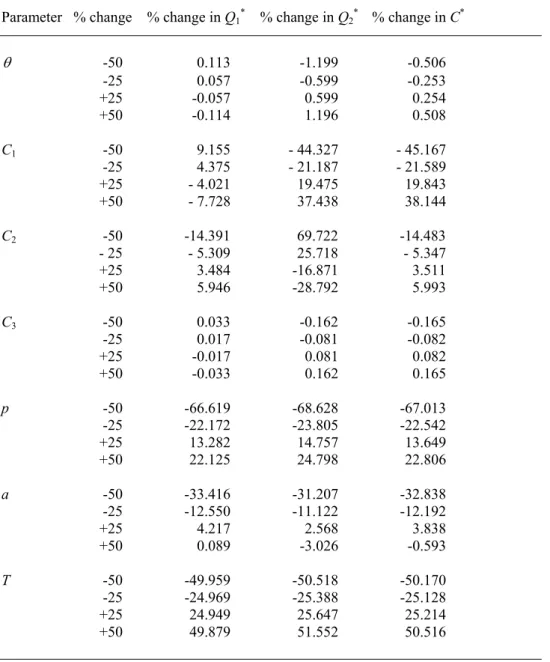
Table 1: Sensitivity analysis

Parameter % change % change in Q1* % change in Q2* % change in C*

θ -50 0.113 -1.199 -0.506

-25 0.057 -0.599 -0.253

+25 -0.057 0.599 0.254 +50 -0.114 1.196 0.508

C1 -50 9.155 - 44.327 - 45.167

-25 4.375 - 21.187 - 21.589 +25 - 4.021 19.475 19.843 +50 - 7.728 37.438 38.144

C2 -50 -14.391 69.722 -14.483

- 25 - 5.309 25.718 - 5.347 +25 3.484 -16.871 3.511 +50 5.946 -28.792 5.993

C3 -50 0.033 -0.162 -0.165

-25 0.017 -0.081 -0.082 +25 -0.017 0.081 0.082 +50 -0.033 0.162 0.165

p -50 -66.619 -68.628 -67.013

-25 -22.172 -23.805 -22.542 +25 13.282 14.757 13.649 +50 22.125 24.798 22.806

a -50 -33.416 -31.207 -32.838

-25 -12.550 -11.122 -12.192 +25 4.217 2.568 3.838 +50 0.089 -3.026 -0.593

T -50 -49.959 -50.518 -50.170

-25 -24.969 -25.388 -25.128 +25 24.949 25.647 25.214 +50 49.879 51.552 50.516

II. We now study the effects of changes in the values of the parameters θ, C1, C2, C3, p, a, and Q1 on the optimal total inventory cost , cycle time and backlog level by using example 2 .

Table 2: Sensitivity analysis

Parameter % change %change in T* % change in Q2* % change in C*

θ -50 0.187 1.960 0.244

-25 0.094 0.981 - 0.122

+25 -0.094 -0.981 0.123

+50 -0.188 -1.974 0.248

C1 -50 -4.515 -53.646 -48.639

-25 -2.231 -26.513 -42.056

+25 2.183 25.934 23.561

+50 4.319 51.326 46.657

C2 -50 11.400 135.458 -3.823

-25 3.939 46.805 -1.400

+25 -2.439 -28.989 0.973

+50 -4.100 -48.725 1.731

C3 -50 -1.625 -19.311 0.028

-25 -0.809 - 9.616 -0.024

+25 0.803 9.538 0.097

+50 1.599 19.002 0.264

p -50 222.603 84.082 2.465

-25 33.414 43.977 0.600

+25 -15.165 -45.479 1.040

+50 -24.595 -92.649 4.122

a -25 8.876 -55.540 1.555

+25 0.141 50.706 0.800

+50 8.256 97.018 3.158

+75 27.850 139.245 6.520

Q1 -50 -49.107 -39.536 -49.973

-25 -24.328 -17.116 -25.012

+25 23.869 11.741 25.135

+50 47.275 18.030 50.469

Therefore the above sensitivity analysis indicates that sufficient care should be taken to estimate the parameters C1, C2, p, a and T(or Q1) in market studies.

6. CONCLUDING REMARKS

In the present paper, we have dealt with a continuous production control inventory model for deteriorating items with shortages. It is assumed that the demand and production rates are constant and the distribution of the time to deterioration of an item follows the exponential distribution. This model is applicable for food items, drugs, pharmaceuticals etc. Here we have studied the structural properties of this inventory system. The sensitivity analysis shows that sufficient care should be taken to estimate the parameters C1, C2, p, a and T (or Q1) in market studies.

Acknowledgement: The authors would like to thank the referee for helpful comments.

REFERENCES

[1] Aggarwal, S.P., A note on an order-level inventory model for a system with constant rate of deterioration, Opsearch, 15 (1978) 184-187.

[2] Bahari-Kashani, H., "Replenishment schedule for deteriorating items with time-proportional demand", Journal of the Operational Research Society, 40 (1989) 75-81.

[3] Covert, R.P., and Philip, G.C., "An EOQ model for items with Weibull distribution deterioration", AIIE Transaction, 5 (1973) 323-326.

[4] Dave, U., "An order-level inventory model for deteriorating items with variable instantaneous demand and discrete opportunities for replenishment", Opsearch, 23 (1986) 244-249.

[5] Dave, U., and Patel, L.K., "(T,Si) policy inventory model for deteriorating items with time proportional demand", Journal of the Operational Research Society, 32 (1981) 137-142.

[6] Deb, M., and Chaudhuri, K.S., "An EOQ Model for items with finite rate of production and variable rate of deterioration", Opsearch, 23 (1986) 175-181.

[7] Ghare, P.M., and Schrader, G.P., "A model for exponentially decaying inventories", Journal

of Industrial Engineering, 14 (1963) 238-243.

[8] Goswami, A., and Chaudhuri, K.S., "An EOQ model for deteriorating items with shortages and a linear trend in demand", Journal of the Operational Research Society, 42 (1991) 1105-1110.

[9] Goswami, A., and Chaudhuri, K.S., "Variations of order-level inventory models for deteriorating items", International Journal of Production Economics, 27 (1992) 111-117.

[10] Jalan, A.K., and Chaudhuri, K.S., "Structural properties of an inventory system with deterioration and trended demand", International J. of Systems Science, 30 (1999) 627-633.

[11] Mishra, R.B., "Optimum production lot-size model for a system with deteriorating inventory",

International Journal of Production Research, 13 (1975) 495-505.

[12] Nahmias, S., "Perishable inventory theory: A review", Operations Research, 30 (1982) 680-708.

[13] Philip,G.C., "A generalized EOQ model for items with Weibull distribution deterioration",

AIIE Transaction, 6 (1974) 159-162.

[14] Rafaat, F., "Survey of literature on continuously deteriorating inventory model", Journal of

the Operational Research Society, 42 (1991) 27-37.

[15] Shah, Y.K., and Jaiswal, M.C., "An order-level inventory model for a system with constant rate of deterioration", Opsearch, 14 (1977) 174-184.