Fuzzy economic production quantity model with time dependent demand rate

Copyright: Wyższa Szkoła Logistyki, Poznań, Polska

Citation: Indrajitsingha S.K., Routray S.S., Paikray S.K., Misra U., 2016, Fuzzy economic production quantity model with

LogForum

http://www.logforum.net p-ISSN 1895-2038

2016, 12 (3), 193-198

DOI: 10.17270/J.LOG.2016.3.1

e-ISSN 1734-459X

FUZZY ECONOMIC PRODUCTION QUANTITY MODEL WITH TIME

DEPENDENT DEMAND RATE

Susanta Kumar Indrajitsingha

, Sudhansu Sekhar Routray

, Susanta Kumar

Paikray

, Umakanta Misra

1) Berhampur University, Odisha, India, 2) Ravenshaw University, Cuttack, Odisha, India, 3) VSSUT, Burla, Odisha, India, 4) NIST, Golanthara, Berhampur, Odisha, India

ABSTRACT. Background: In this paper, an economic production quantity model is considered under a fuzzy environment. Both the demand cost and holding cost are considered using fuzzy pentagonal numbers. The Signed Distance Method is used to defuzzify the total cost function.

Methods: The results obtained by these methods are compared with the help of a numerical example. Sensitivity analysis is also carried out to explore the effect of changes in the values of some of the system parameters.

Results and conclusions: The fuzzy EPQ model with time dependent demand rate was presented together with the possible implementation. The behavior of changes in parameters was analyzed. The possible extension of the implementation of this method was presented.

Key words: Inventory, Pentagonal Fuzzy Number, Signed Distance Method.

INTRODUCTION

In real-life situations, exact data are often inadequate for a mathematical model. Inventory is a physical stock that a business keeps on hand in order to promote the smooth and efficient running of its affairs. But in practice, the effects of deterioration, shortages, holding cost, ordering cost etc. are important for inventory. Various types of uncertainties are involved in any inventory system. Historically, probability theory has been the primary test for representing uncertainty in mathematical models. Because of this, all the uncertainty was assumed to follow the characteristics of random uncertainty. A random process was one where the outcome of any particular realization of the process is strictly a matter of chance, and prediction of a sequence of events is not possible. Fuzzy set theory is an excellent tool for modeling the

kind of uncertainty associated with vagueness, imprecision and the lack of information regarding a particular problem at hand.

Initially, L.A. Zadeh [1963] introduced the concept of fuzzy sets. In this area a lot of research papers have been published by several researchers viz. S. K. Goyal [1985], Z.T. Balkhi [1998], K.J. Chung[2000], T. Chang [2003], Huang [2007], G.C. Mahata and A. Goswami [2010], S. K. Indrajitsingha et. al. [2015].

DEFINITIONS AND

PRELIMINARIES

In order to treat a fuzzy inventory model by using the graded mean representation method to defuzzify, we need the following definitions.

Definition 2.1 (Fuzzy Set) Let be a space of points with a generic element of . Let

: ⟶ [0,1] be such that for every ∈ ,

( ) is a real number in the interval [0,1], usually called ‘ grade of membership’. We define a fuzzy set in as the set of points

= { , ( ) : ∈ }.

Definition 2.2 (Convex Fuzzy Set) A fuzzy set = { , ( ) } ⊆ is called convex fuzzy set if all are convex sets for every ∈ . That is, for every pair of

elements _, ∈ and ∈ [0,1], +

(1 − ) ∈ , ∀ ∈ [0,1]. Otherwise the fuzzy set is called a non-convex fuzzy set.

Definition 2.3 A fuzzy set [" , # ] where

0 ≤ ≤ 1 and " < # defined on &, is called a fuzzy interval if its membership function is

['(,)(]= * , " ≤ ≤ #0 , +,ℎ./012.

Definition 2.4 A fuzzy number =

(", #, 3, 4, .) where " < # < 3 < 4 < . defined on R, is called pentagonal fuzzy number if its membership function is

=

5 66 6 7 66 6

89 ( ) =# − " , " ≤ ≤ #− " 9 ( ) = − #_{3 − # , # ≤ ≤ 3} 1, = 3 & ( ) = 4 −_{4 − 3 , 3 ≤ ≤ 4} & ( ) = . −_{. − 4 , 4 ≤ ≤ .}

0, +,ℎ./012.

Then − 3:, of = (", #, 3, 4, .), 0 ≤

≤ 1 is ( ) = [ ;( ), <( )].

Where _;=( ) = " + (# − ") = 9 > ( )

;?( ) = # + (3 − #) = 9 > ( )

< ( ) = 4 − (4 − 3) = & > ( )

<?( ) = . − (. − 4) = & > ( )

9> _{( ) =}9 > ( ) + 9 > ( ) 2

=" + # + (3 − ")₂

&> _{( ) =}& > ( ) + & > ( ) 2

=4 + . − (. − 3)₂

Definition 2.5 If = (", #, 3, 4, .) is a pentagonal fuzzy number then signed distance method of is defined as

4 , 0 = A 4([ ;( ), <( )], 0) B

=1_{8 (" + 2# + 23 + 24 + .)}

ASSUMPTIONS

The following assumptions are made throughout the manuscripts:

1.Items are produced and added to the inventory.

2.The lead time is zero.

3.Two rates of production are considered. 4.No shortage is allowed.

5.The production rate is proportional to the demand rate.

6._{The production rate is always greater than}

the demand rate.

NOTATIONS

4(,) = " + #,, " > 0, 0 < # < 1.

E(,) = inventory level at any time′,′.

F = production rate in units per unit time.

4 = demand rate in units per unit time.

EB = on hand inventory level during [0, G ]. Q = production quantity.

H = production cost per unit.

I = holding cost per unit time.

I = setup cost per setup.

ℎJ= holding cost per unit time. GJ = total cost.

G = cycle time.

G = production time.

KI = setup cost.

4 = fuzzy demand.

I = fuzzy holding cost per unit time.

GJ = total fuzzy inventory cost per unit time.

LM= production quantity in the Signed

Distance Method.

GJM= defuzzifying value of GJ by applying

Signed Distance method.

MATHEMATICAL FORMULATION

In this model it is assumed that the production starts with a rate F , at , = 0 and is stopped at , = G > 0. It is also assumed that from the starting itself the demand is met. As

F is assumed as F = O4 , O > 1 , during the interval [0, G ] , the inventory accumulates at a rate F − 4. During the interval [G , G ], there is no production and only the inventory is consumed as per the demand till it becomes zero at , = G .Thus the rate of change of inventory is governed by the differential equations.

CRISP MODEL

(5.1)4E(,)_{4, = F − 4 ; 0 ≤ , ≤ G}

and

(5.2)4E(,)_{4, = −4 ; G ≤ , ≤ G}

where

4 ≡ 4(,) = " + #,, " > 0, 0 < # < 1, F = O4 "S4 O > 1.

Solution of (5.1) and (5.2) with the condition E(0) = 0, E(G ) = EB, E(G) = 0, and

G = G + G is given by

(5.3) E(,) = (O − 1) U" +#,_{2 V , , 0 ≤ , ≤ G}

and from (5.2)

4E(,)

4, = −(" + #,) A 4E(,) = − A(" + #,)4,

E(,) = − U" +#,_{2 V , + W,}

0here K is a constant of integration.

With condition I (T) =0, we get

W = "G +#G₂

Hence we have

(5.4) E(,) = "(G − ,) +#_{2 (G − , )}

At , = G (5.3) and (5.4) are same i.e.,

(5.5)EB= (O − 1) U" +#G_{2 V G} = "G +# G_{2 G + 2G}

At , = 0, the order quantity

(5.6) L = "G +#G₂

(5.7) G =[" + 2#L − "_#

The total cost is calculated by considering the setup cost, production cost and inventory holding cost:

1.Setup cost KI =\_]?= )\?

['?_{^ )_>'}

2.Production cost F_J=`a]<sub>]</sub>==`(" +

[" + 2#L)

3.Inventory holding cost

ℎJ =_{2G [(O − 1) U" +}I #G_{3 V G}

+" G − G +#_{3 (G − G )(2G + 2G} + 5G G )]

The total cost is

(5.8) GI = KI + FJ+ ℎJ = #(I + I )

[" + 2#L − "+ F 2 (" + [" + 2#L)

where

= [(O − 1) b" +)]=

c d G + " G − G +)_c(G − G )(2G + 2G + 5G G )]

FUZZY MODEL

Let "e = (" , " , "c, "f, "g) ,# = (# , # , #c, #f, #g), I = (ℎ , ℎ , ℎc, ℎf, ℎg) are pentagonal fuzzy numbers.

The total cost of the system per unit time in the fuzzy environment is given by

(5.9)GJ = #I ["i + 2#L − "i

+ I

["i + 2#L − "ij(O − 1) k"i + #G

3 lG + "i G − G +#_{3 (G − G ) 2G + 2G + 5G G m +}F_{2 ("i +}n"i + 2#L)

We defuzzify the fuzzy total cost G_J by the Signed Distance Method. By the Signed Distance Method, the total cost is given by

GJM=1_{8 [G}JM + 2GJM + 2GJMc+ 2GJMf+ GJMg]

Where

GJM = # I

[" + 2# L − " +

ℎ

2[" + 2# o − " [(O − 1) U" + # G

3 V G + " G − G +#_{3 (G − G )(2G + 2G + 5G G )]}

GJM = # I

[" + 2# L − " +

ℎ

2[" + 2# L − " [(O − 1) U" + # G

3 V G + " G − G +#_{3 (G − G )(2G + 2G + 5G G )]}

GJMc= #cI

["c + 2#cL − "c+

ℎc

2["c + 2#cL − "c[(O − 1) U"c+ #cG

3 V G + "c G − G +#c_{3 (G − G )(2G + 2G + 5G G )]}

GJMf= #fI

["f + 2#fL − "f+

ℎf

2["f + 2#fL − "f[(O − 1) U"f+ #fG

3 V G + "f G − G +#f_{3 (G − G )(2G + 2G + 5G G )]}

GJMg= #gI

["g + 2#gL − "g+

ℎg

2["g + 2#gL − "g[(O − 1) U"g+ #gG

3 V G + "g G − G +#g_{3 (G − G )(2G + 2G + 5G G )]}

NUMERICAL EXAMPLE

Consider the inventory system with the following parametric values:

CRISP MODEL

" = 1000 unit/year, O = 1.3, # = 0.2 unit/year, I = 20, I = 2 per unit/year, F =

20 units, G = 0.3 year, G = 0.36 year.

The solution of the crisp model is

GJ = &2. 20033, L = 660.04.

FUZZY MODEL

"i = (600,800,1000,1200,1400), # = (0.16,0.18,0.20,0.22,0.24),

I = (1,1.5,2,2.5,3)

Total cost is G_JM = &2. 20033.63, and LM= 660.04.

SENSITIVITY ANALYSIS

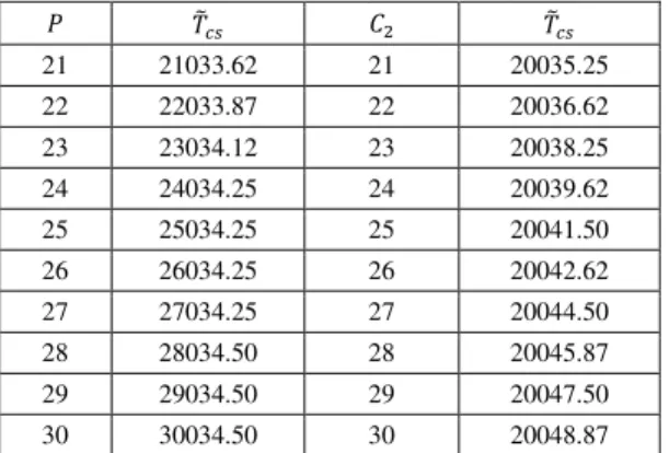
A sensitivity analysis is performed to study the effects of changes in parameters P and C2.

Table 1. Results of the sensitivity analysis Tabela 1. Wyniki analizy wrażliwości

F GJM I GJM

21 21033.62 21 20035.25

22 22033.87 22 20036.62

23 23034.12 23 20038.25

24 24034.25 24 20039.62

25 25034.25 25 20041.50

26 26034.25 26 20042.62

27 27034.25 27 20044.50

28 28034.50 28 20045.87

29 29034.50 29 20047.50

30 30034.50 30 20048.87

From the above observation we have concluded as follows:

− As the value of C2 increases, the fuzzy total

cost G_JM increases.

− As the value of P increases, the fuzzy total cost G_JM increases.

In the cases of both production cost and setup cost, the fuzzy total cost increases more in event of an increase in production cost as compared to an increase in the setup cost.

CONCLUSION

This paper presents a fuzzy EPQ model with a time-dependent demand rate. The demand and setup cost is represented by pentagonal fuzzy numbers. To evaluate the total fuzzy cost the Signed Distance Method was used. A sensitivity analysis was also conducted to determine the behavior of changes in parameters. For instance, we may extend this model to use a graded mean representation method and centroid method etc.

ACKNOWLEDGEMENTS

The first author would like to acknowledge the DST for providing DST INSPIRE fellowship vide letter no. DST/INSPIRE

Fellowship/2014/281 with diary No.

C/4588/IFD/2014-15.

REFERENCES

Zadeh, L.A., 1963. Fuzzy Sets, Information and Control, 8(3), 338-353.

Goyal, S.K., 1985. Economic order quantity under conditions of permissible delay in payments, Journal of Operation Research Society, 36, 335-338.

Balkhi, Z.T., 1998. On the global optimality of a general deterministic production lot size inventory model for a deteriorating item, Belgian J. Oper. Res, Statistics Comput. Sci., 33-44.

Chung, K.J., 2000. The inventory replacement policy for deteriorating items under permission delay in payments, Oper. Res., 267-281.

Chang, C.T., Ouyang, L.Y., Teng J.T., 2003. An EOQ model for deteriorating items under supplier credits linked to ordering quality, Appl. Math. Model, 27, 983-996.

Huang, Y.F., 2007. Optimal retailor's replenishment decisions in the EPQ model under two levels of trade credit policy, European J. Oper. Res., 176, 1577-1591.

Mahata, G.C., Goswami, A., 2010. The optimal cycle for EPQ inventory model of deteriorating items under trade credit financing in the fuzzy sense, International Journal of Operations Research, 7(1), 27-41.

MODEL ROZMYTEJ EKONOMICZNEJ WIELKO

Ś

CI PRODUKCJI

FUNKCJI POPYTU ZALE

Ż

N

Ą

OD ZMIENNEJ CZASU

STRESZCZENIE. Wstęp: W pracy przedstawiono model ekonomicznej wielkości produkcji w rozmytym otoczeniu. Zarówno koszy popytu jak i koszt utrzymania zapasu zostały ujęte, jako rozmyte liczby pentagonalne. Metoda Signed Distance została użyta w celu uszczegółowienia funkcji kosztu całkowitego.

Metody: Wyniki otrzymane w obu metodach zostały ze sobą porównane w przykładzie liczbowym. Przeprowadzono analizę wrażliwości w celu określenia wpływu niektórych parametrów na zmiany otrzymywanych wartości.

Wyniki i wnioski: Zaprezentowano model ekonomicznej wielkości produkcji funkcji popytu zależnej od zmiennej czasu wraz z możliwym jej zastosowaniem. Przeanalizowano zależności zmian wielkości parametrów. Zaproponowano możliwe rozszerzenie zastosowania tej metody.

Słowa kluczowe:zapas, rozmyta liczba pentagonalna, metoda Signed Distance.

EIN

MODELL

FÜR

DIE

WIRTSCHAFTLICHE

FUZZY-PRODUKTIONSGRÖßE

IN

BEZUG

AUF

DIE

VON

DER

ZEITVARIABLE ABHÄNGIGEN NACHFRAGEFUNKTION

ZUSAMMENFASSUNG. Einleitung: Im vorliegenden Beitrag wurde ein Modell für die wirtschaftliche Produktionsgröße im Fuzzy-Umfeld dargestellt. Sowohl die Nachfragekosten, als auch die Kosten der Vorratshaltung wurden als Fuzzy-Pentagonalzahlen angeführt. Die Signed Distance-Methode wurde zwecks einer Detaillierung der auf die Gesamtkosten bezogene Funktion angewendet.

Methoden: Die bei der Anwendung der beiden Methoden erzielten Ergebnisse wurden in einem Zahlenbeispiel miteinander verglichen. Es wurde eine Sensitivitätsanalyse zwecks der Ermittlung des Einflusses mancher Parameter auf die Veränderung der erzielten Werte durchgeführt.

Ergebnisse und Fazit: Es wurde ein Modell für die wirtschaftliche Produktionsgröße in Bezug auf die von der Variable der Zeit abhängigen Nachfragefunktion samt deren möglichen Anwendung dargestellt. Es wurden Abhängigkeiten innerhalb von Veränderungen der betreffenden Parameterwerte analysiert sowie eine mögliche Verbreitung der Anwendung dieser Methode vorgeschlagen.

Codewörter: Vorrat, Fuzzy-Pentagonalzahl, Signed Distance-Methode

Susanta Kumar Indrajitsingha

DST INSPIRE Fellow, P.G. Department of Mathematics Berhampur University, Odisha, India

e-mail: skismath86@gmail.com

Sudhansu Sekhar Routray

Research Scholar, Dept. of Mathematics Ravenshaw University

Cuttack, Odisha, India

e-mail: sudhansu31@gmail.com

Susanta Kumar Paikray Dept. of Mathematics, VSSUT Burla, Odisha, India

e-mail: spaikray2001@gmail.com

Umakanta Misra

Dept. of Mathematics, NIST