ABSTRACT:Fish consumption per capita in Brazil is relatively modest when compared to other animal proteins. This study analyses the influence of protein prices, other food prices and population income on the fish demand in Brazil. First, the problem of fish supply in Brazil is characterized. It is followed by reviews of the relevant economic theory and methods of Almost Ideal Demand System- AIDS and their elasticity calculations. A descriptive analysis of fish de-mand in Brazil using the microdata called “Pesquisa de Orçamento Familiar” (Familiar Budget Research) - POF 2002-2003 is presented. Finally, demand functions and their elasticities are calculated for two different cases: one considering five groups of animal proteins (Chicken; Milk and Eggs; Fish; Processed Proteins and Red Meat) and other with seven groups of food categories (Cereals; Vegetables and Fruits; Milky and Eggs; Oils and Condiments; Fish; Other processed foods; and Meats). The main results are: per capita consumption of fish (4.6 kg per inhabitant per year) is low in Brazil because few households consume fish. When only house-holds with fish consumption are considered, the per capita consumption would be higher: 27.2 kg per inhabitant per year. The fish consumption in the North-East Region is concentrated in the low-income class. In the Center-South Region, the fish consumption is lower and concen-trated in the intermediate income classes. The main substitutes for fish are the processed proteins and not the traditional types of meat, such as chicken and red meat.
Keywords: AIDS, fish, supply, elasticity, market
Introduction
The world fishery production decreased steadily from the early 1960s to the 1990s, when it stabilized at about 80 million tonnes per year. Since the 1970s, aquaculture has increased its share in the total fish pro-duction and since the mid-1980s was the only source of growth in the total global production (FAO, 2005). In Brazil, fishery production increased until 1985 reach-ing one million ton per year. The national production fell abruptly in 1986 with the end of governmental in-centives to the industry and then remained constant at around 0.7 million ton until the end of the 1990s (Abdallah and Bacha, 1999).
Since the 1970s, technological advances in tradi-tional substitutes for fishery products in the food mar-ket, namely beef, pork and poultry industries, resulted in a continuous price reduction of those products in Brazil, whereas the price of fishery products did not decrease in the same period (Sonoda et al., 2002). As
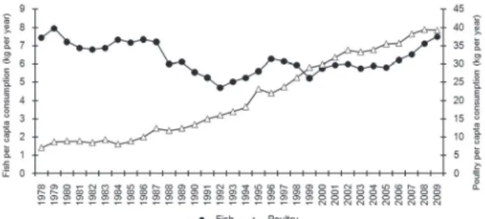
a consequence, fish lost its price competitiveness with other meats (Figure 1).
The impact of these developments on the fish
mar-ket was quite significant: while per capita consumption
of fish decreased from 8 to 5 kg per year between 1978 and 2003, poultry consumption increased sharply from 7 to 34 kg per year in the same period (Figure 2) (ABEF, 2005). This trend could be changed by increasing the supply of fishery products which would benefit pro-ducers and promote healthier food for the population. However, when t demand for fish increases, it is neces-sary to understand the relative demand for this product regarding other groups. These answers are important to guide public and private national fishery development processes and plan the growth of its production, indus-trial and distribution sectors.
This study aims to estimate demand functions for fishery products in Brazil and to calculate compensated and uncompensated price elasticity for animal protein being fish, red meats, poultry, milk and eggs, and
pro-Received April 09, 2010 Accepted February 14, 2012
1PECEGE, R. Alexandre Herculano, 120,
sala T-4 – 13418-445 – Piracicaba, SP – Brasil.
2Embrapa Estudos e Capacitação (CECAT), Parque Estação
Biológica – PqEB s/n – 70770-901 – Brasília, DF – Brasil.
3USP/ESALQ – Depto. de Zootecnia,
C.P. 09 – 13418-900 – Piracicaba, SP – Brasil.
4USP/ESALQ – Depto. de Economia, Administração e
Sociologia.
*Corresponding author <[email protected]>
Edited by: Gerson Barreto Mourão
Demand for fisheries products in Brazil
Daniel Yokoyama Sonoda1*, Silvia Kanadani Campos2, José Eurico Possebon Cyrino3,Ricardo Shirota4
Figure 1 – Brazil: Prices of wholesale cattle, pork and poultry meat of Dec/09. 1989–2009.
cessed proteins; other foods such as cereals, fruit and vegetables, milk and eggs, oils and condiments, fish, other processed foods, and meats.
Materials and Methods
Almost Ideal Demand System-AIDS is a system of equations that belongs to a class denominated piglog functions. It defines the minimum cost (or expenditure) required to attain a certain utility level, known the pric-es. The piglog was, originally, represented by a cost
func-tion c(u, p), where u represents utility and p the vector of
prices (Deaton and Muellbauer, 1980):
ln ( , ) (1c u p = −u)ln[ ( )]a p +uln[ ( )]b p (1)
The utility level is delimited between zero and one
(0 ≤ u ≤ 1), where 0 (zero) represents the subsistence
level and 1 (one) represents the limit of satisfaction for the consumption. These functions are linearly
homoge-neous and positive in a(p) and b(p). The functional forms
of a(p) and b(p)are usually expressed by:
* 0
1
ln ( ) ln ln ln
2 j
k k kj k
k k j
a p =α +
∑
α p +∑∑
γ p p ( 2 )0
ln ( ) ln ( ) k k k b p = a p+β
∏
pβ
(3)
The AIDS cost function becomes:
*
0 0
1
ln ( , ) ln ln log
2
k j
k k kj k k
k k j k
c u p =α +
∑
α p +∑∑
γ p p +uβ∏
pβ (4)where, αi, βiand γ*
ij are parameters.
The expenditure share of good I (wi ) derivate from
ln c(u,p) in terms of ln pi is given by (Griliches and Intrili-gator, 1990):
0
1 1
ln ln
2 2
k
i i kj k kj j i k
k j
w =α +
∑
γ p +∑
γ p +uβ βΠp βln k
o
i i ij j i k
j
w = +a
∑
γ p +β βu∏
pβ (5)* * 1
( )
2 ij ij ji
γ = γ +γ (6)
Expressing wi in terms of expenditure of good i
(adapted from Silberberg, 1990):
ln ln
i i ij j i
j
x
w p
P
α γ β
= +
∑
+ (7)where P is a price index:
0
1
ln ln ln ln
2 j
k k kj k
k k j
P=α +
∑
α p +∑∑
γ p p (8)Taking restrictions (9), (10) and (11) into account, and assuming that (7) represents a system of equations
where
∑
wi=1 (additive condition), the demand modelis homogeneous of degree 0 (zero) for prices and income, and satisfies the Slutsky symmetry. In absence of
varia-tion in the relative prices (p) and the real income (x/P),
the expenditure share (wi) remains constant. Changes in
the real income modify βi and its sum in i is 0 (zero).
The positive values of βi represents luxury goods and the
negative ones, subsistence goods.
1
1
n
i i
α =
=
∑
1
0
n
ij i
γ =
=
∑
1
0
n
i i
β =
=
∑
(9)0
ij j
γ =
∑
(homogenity) (10)ij ji
γ =γ (symmetry) (11)
A better approximation of wi could be achieved
generalizing (7) for a individual household, h:
ln ln h
i ij j i
ih
j h
x
w p
k P
α γ β
= +
∑
+(12)
Parameter kh is interpreted as a measure of
house-hold size and reflects an adjustment for an “adult coef-ficient” of food consumption that takes into account the age and gender of its members. This parameter is used
to correct or to weight the per capita income xh (Deaton
and Muellbauer, 1980). If the household members were homogeneous in terms of food consumption, the
param-eter kh could be represented by the number of resident
people in household h. However, household components
are generally heterogeneous in terms of age and gender,
for instance. Thus, kh makes an adjustment for this
fac-tor that affect food consumption, to a relative value of “adult equivalent”. For example, a child or adolescent is considered a fraction of an adult male. The Amsterdam
Scale (Stone, 1954 apud Deaton and Muellbauer, 1986),
based on the nutritional requirement of people, is an em-pirical application of this method (Table 1). A household represented by one man, one woman and a couple of children (< 14 years), has the “adult equivalent” of 2.94
instead of 4.0 if this per capita index was considered.
There are two alternative methods of estimation. First, a nonlinear system using maximum likelihood, which follows by substituting (8) in (7):
0
1
( ) ln ln ln ln ln
2
α β α γ β α γ
= − +
∑
+ −∑
−∑∑
i i i ij j i k k kj k j
j k k j
w p x p p p
(13)
Table 1 – Amsterdam Scale, adapted from Deaton e Muellbauer (1986).
Age Male Female
< 14 years 0.52 0.52
from 14 to 17 years 0.98 0.90
The main problem with this approach is the
identification of parameter α0 (Deaton and
Muellbau-er, 1980). Alternatively, such as in this study, these equations could be estimated by Seemingly Unre-lated Regressions (SUR) using ordinary least square
(OLS) if P in (7) were linear in terms of parameters
α, β and γ.
In a situation where prices are closely collinear, P
could be known as an index price P* (Stone, 1954 apud
Deaton and Muelbauer, 1980):
*
lnP =
∑
wklnpk(14)
The same index was used to calculate the prices pj
in (7) and (8). If P ≅φP*, then equation (7) can be
writ-ten as:
*
( log ) ln ln
i i i ij j i
j
x
w p
P
α β ϕ γ β
= − +
∑
+(15)
considering αi* = α
i - βi logφ and
* 0
k
α =
∑
, if∑
βk=0.In eq. (15) if high income households consume the same amount of food as the low income households, but their expenditures are higher as a result of prices differences, results could be understood as a proxy to the quality associated to the food products consumed.
Therefore, x/P* represents the amount weighed for the
quality of food product per household. Uncompensated price elasticities in AIDS functions are calculated from eq. (8) as follows (Alston et al., 1994):
ln ln
ln ln
i
i i i i i
ij ij ij ij
j
j j i i
j w
q w w w p
p
p p p w
p
ε δ δ δ
∂
∂ ∂ ∂
= = − + = − +∂ = − + ⋅
∂ ∂ ∂
(
i ijln j iln iln)
j ij ijj i
p x P p
p w
α γ β β
ε = − +δ ∂ + + − ⋅
∂
∑
0 kln k 12 kjln kln j k j
ij j
ij ij i
j j i
p p p
p
p p w
α α γ
γ
ε δ β
∂ + +
= − + −
∑
∂∑∑
⋅ln ln
1 1
2 2
ij j k k j
ij ij i kj kj
k j
j j j j i
p
p p
p p p p w
γ α
ε δ β γ γ
= − + − ⋅ +
∑
+∑
⋅1
ln n ij i
ij ij j kj k
k
i i
p w w
γ β
ε δ α γ
=
= − + − ⋅ +
∑
(16)
where, δij is Kronecker delta (δij = 1 if i = j and δij = 0
if i ≠ j).
Compensated price elasticities (ε*
ij) are calculated
using Slutsky equation:
*
,
ij ij wj i x
ε =ε + ε
(17)
where: ei,x is expenditure elasticity for good i.
, 1 i
i x i w
β
ε = +
(18)
Therefore, compensated price elasticity for AIDS function is given by:
*
1
ln
n
ij i
ij ij j j kj k j
k
i i
w p w
w w
γ β
ε δ α γ
=
= − + + − +
∑
−(19)
The elasticities can be calculated by a linear
ap-proximation (Chalfant, 1987 apud Alston, 1994).
Consid-ering a special case of derivation of P* from (14):
*
j j P
w p
∂ =
∂
(20)
The linear approximation of eij(AL) ande*
ij(AL):
( ) ij i
ij ij j
i i
AL w
w w
γ β
ε = − +δ − ⋅
(21)
*
( ) ij
ij ij j
i
AL w
w
γ
ε = − +δ +
(22)
The study uses data from “Pesquisa de Orçamento Familiar” [POF] (Household Budget Research) from 2002-2003 (IBGE, 2004) which contains information about the expenditure of a sample of 48,471 Brazilian households. Data was collected from July 2002 to June 2003 and is the most recent data available. All the expenses were registered for one week in each household in the sample. The data set covers all geographic regions and economic stratum with prices adjusted to 01 Mar., 2003.
In order to understand the demand function better, data was grouped and analyzed in two alternative forms. First, non-processed fish consumption was compared with the consumption of other animal protein. “Protein” demand was divided into five categories: fish, red meats, chicken, milk and eggs, and processed proteins. The first four categories represent purchases of proteins of low level processing (chilled, frozen or salted meat (whole or in cuts) or live animals) and the last includes these four proteins purchased by households but with higher degrees of processing.
The second analysis considers wider consump-tion categories ignoring the degree of processing. Foods were separated into seven groups namely cereals, fruit and vegetables, milk and eggs; oils and condiments; fish, other processed foods, and other meats. Here though, processed proteins were placed in their respective fish, milk and egg, and total meat categories.
custom-er defines what fraction of their income will be allocat-ed to the purchase of animal protein and subsequently chooses products based on relative prices. It is worth noting that in the estimation of compensated price elas-ticity of demand, the omission of the outside alternative in conjunction with the usual restrictions (symmetry of the Slutsky matrix, the sum of shares equal to 1, etc. ...), tends to exaggerate the income effect and this tendency is proportional to the expenditure share of the good in the total expenditure.
The data line was considered in the model only when the budget share of all categories (five for Proteins and seven for Food) was more than zero, otherwise it was deleted.
Results and Discussion
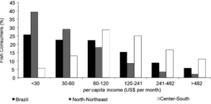
Figure 3 shows the income distribution in Brazil, in total and by regions. In the North-Northeast Region, the population is concentrated in lower income levels whereas in the Central-South the concentration is inter-mediate levels of income. Interesting enough, fish con-sumption has a similar distribution (Figure 4).
Overall, the per capita consumption of 4.59 kg per
yearof fish is quite low in comparison with other
coun-tries. However it is clear that this results from the fact that few individuals (only 29.6 million people out of 175
million report fish consumption) eat a good quantity of fish. This number needs increasing and not just among
current consumers. The per capita consumption rises up
to 27.22 kg per year when one considers only fish con-sumers. The consumption pattern also varies between regions. In the North and Northeast Regions, 28 % of the population eats fish while in the Central-South that ratio drops to 11 %. As a consequence, 60 % of fish consumers are in the North-Northeast Region and 40 % are located in the Central-South.
The third fact worth mentioning is the proportion of households reporting fish consumption: 11,296 out of 48,471 in the sample, and only 1,324 households report-ing simultaneous consumption of all five animal protein categories. This scenario could be explained by the facts that: (i) the household consumes all animal proteins but some (or all) of these were not consumed in the survey week; (ii) the household does not have the habit of con-suming either a little (or any) animal protein; and, (iii) for some reason (unknown), the information regarding this amount (kg) consumed is absent.
In the first model, AIDS function was applied to the five animal protein categories, represented by: a - chicken; l - milk and eggs; p - fish; t - processed proteins; and, v - red meats. Another three important abbreviations for the understanding of these
func-tions are: wi – expenditure share of protein, i (out of
x- total expenditure in animal protein); lpi – Neperian
logarithms of i-th animal protein price; and x/kP –
Ne-perian logarithms of expenditure with animal proteins divided by the adult index equivalent in the household
(k) times the price index (P). The percentage of
expen-diture on animal protein per category (wti) of POF was
compared with the same percentage of expenditure to the group of 5 protein categories consumed
simultane-ously (wi). The main difference was that (wi) consumers
had spent three times more on fish than the national average. The ready protein consumption was
practi-cally the same; however, (wi) consumers had a larger
consumption of chicken and a lesser consumption of red meats, milk and eggs than the national average for meat (Figure 5).
Figure 3 – Brazil: North-Northeast and Center-South Regions: distribution of population according to per capita income. 2003 (source IBGE. 2004).
Figure 5 – Brazil: distribution of animal protein consumption by categories expenditure in “Pesquisa de Orçamento Familiar” (Familiar Budget Research) - POF (wt) and the group of 5 protein categories simultaneously consumed (w). 2003. Original research data. Figure 4 – Brazil: North-Northeast and Center-South Regions:
The estimative results of the model, test t, F and
the low value for R2 were already expected since
cross-section data (Griffiths et al., 1993) (Table 2). The t test
using the restricted model parameters (equations 10, 11 and 12) is better than the partially restricted model (equation 11).
Uncompensated and compensated price elasticity (both sample and cross price data) and income
elastic-ity were estimated from wi and parameter functions.
The signs of most of the price itself and income elastic-ity were consistent with the microeconomic theory. In some cases, the signs for the uncompensated and com-pensated cross price elasticity are the contrary to those expected. This analysis was based on the compensated elasticity and is hence coherent with the microeconomic theory (Table 3). All elasticity in compensated cross price analysis was positive. Curiously, the highest cross price
elasticity was for processed proteins (ε*p
pt) milk and eggs
(ε*p
pl) and not for chicken (ε
*p
pa) or red meat (ε
*p
pv) which
were expected to be the main fish competitors.
Price of fishery products and income elasticity es-timated in this study are similar to those found for Japan (Hayes et al., 1990; Chalfant et al., 1991). Although these studies do not compare the same animal protein groups, all cross elasticity, (USA data excluded), is lower than their prices and income elasticity. Income elasticity estimated for Brazil, Japan and Canada have a stronger influence on fish demand than the surrogate goods (Table 4).
The other model, with seven food categories (c - cereals; h - fruit and vegetables; m - milk and eggs; o - oils and condiments; d - fish; r - other processed foods;
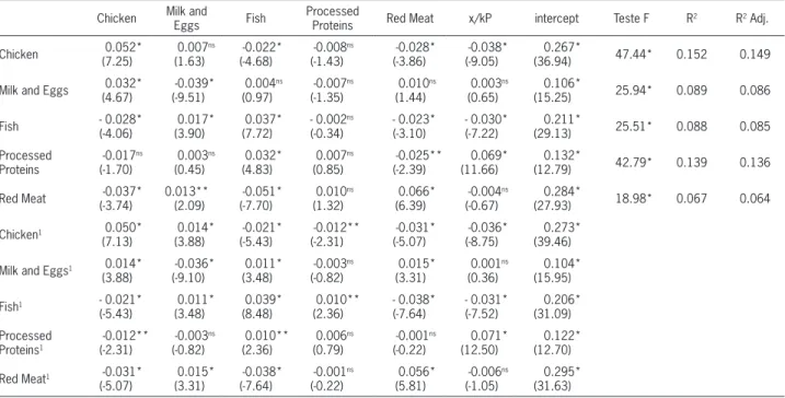
Table 2 –Brazil: parameters and statistic tests estimates for partial restricted and restricted almost ideal demand system - AIDS functions for five animal proteins categories. Original research data; parameters estimated by Neperian logarithm transformation.
Chicken Milk and
Eggs Fish
Processed
Proteins Red Meat x/kP intercept Teste F R
2 R2 Adj.
Chicken (7.25)0.052* 0.007
ns
(1.63)
-0.022* (-4.68)
-0.008ns
(-1.43)
-0.028* (-3.86)
-0.038* (-9.05)
0.267*
(36.94) 47.44* 0.152 0.149
Milk and Eggs (4.67)0.032* (-9.51)-0.039* 0.004
ns
(0.97)
-0.007ns
(-1.35)
0.010ns
(1.44)
0.003ns
(0.65)
0.106*
(15.25) 25.94* 0.089 0.086
Fish - 0.028*(-4.06) (3.90)0.017* (7.72)0.037* - 0.002
ns
(-0.34)
- 0.023* (-3.10)
- 0.030* (-7.22)
0.211*
(29.13) 25.51* 0.088 0.085
Processed Proteins
-0.017ns
(-1.70)
0.003ns
(0.45)
0.032* (4.83)
0.007ns
(0.85)
-0.025** (-2.39)
0.069* (11.66)
0.132*
(12.79) 42.79* 0.139 0.136
Red Meat (-3.74)-0.037* 0.013**(2.09) (-7.70)-0.051* 0.010
ns
(1.32)
0.066* (6.39)
-0.004ns
(-0.67)
0.284*
(27.93) 18.98* 0.067 0.064
Chicken1 0.050*
(7.13)
0.014* (3.88)
-0.021* (-5.43)
-0.012** (-2.31)
-0.031* (-5.07)
-0.036* (-8.75)
0.273* (39.46) Milk and Eggs1 0.014*
(3.88)
-0.036* (-9.10)
0.011* (3.48)
-0.003ns
(-0.82)
0.015* (3.31)
0.001ns
(0.36)
0.104* (15.95)
Fish1 - 0.021*
(-5.43)
0.011* (3.48)
0.039* (8.48)
0.010** (2.36)
- 0.038* (-7.64)
- 0.031* (-7.52)
0.206* (31.09) Processed
Proteins1
-0.012** (-2.31)
-0.003ns
(-0.82)
0.010** (2.36)
0.006ns
(0.79)
-0.001ns
(-0.22)
0.071* (12.50)
0.122* (12.70) Red Meat1 -0.031*
(-5.07)
0.015* (3.31)
-0.038* (-7.64)
-0.001ns
(-0.22)
0.056* (5.81)
-0.006ns
(-1.05)
0.295* (31.63) Note:1 refers to restricted functions;*p < 0.01; **p < 0.05; ***p < 0.1; ns – non significant.
and, n – meats) was estimated using 3,430 households reporting simultaneous consumption of these foods.
The percentage of expenditure per food category (wt) of
POF was compared with the same percentage of expen-diture to the group of seven food categories consumed
simultaneously (wi). Similar to the situation previously
considered, the main difference was that the consumers Table 3 – Brazil: uncompensated (ep) e compensated (e*p) elasticities
for five animal proteins categories. Original research data.
Chiken Milk and
eggs Fish
Processed
proteins Red meat X
εp
p - 0.11* 0.10* - 0.70* 0.12** - 0.20*
ε*p
p 0.02* 0.21* - 0.59* 0.32** 0.02* 0.79*
*p < 0.01; **p < 0.05.
Table 4 – Brazil/Japan/USA/Canada: uncompensated price and income elasticities for fish.
Brazil Japan* USA* Canada**
Chicken - 0.11 0.01 - 0.12 0.19
Cattle - - 0.04 0.19 0.09
Imported Cattle - - 0.04
Pork - - 0.02 0.16 0.09
Red Meat - 0.20 - -
-Milk and Eggs 0.10 - -
-Processed Proteins 0.12 - -
-Fish - 0.70 - 0.70 - 0.23 - 0.37
Income 0.79 0.78 0.15 0.89
sampled (wi) had spent three times more on fish than the national average. The other food consumption was similar to the national average (Figure 6).
The statistical results were similar to the previ-ous model (Table 5). The signs of uncompensated and
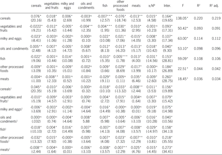
Table 5 – Brazil: almost ideal demand system - AIDS parameters for partial restricted and restricted functions to 7 food categories. Original research data; parameters estimated by Neperian logarithm transformation.
cereals vegetables and fruits milky and eggs oils and condiments fish other processed foods
meats x/kP Inter. F R2 R2 adj.
cereals 0.076* (20.16) 0.018* (5.43) 0.006* (2.69) -0.003ns (-0.99) -0.007*** (-2.57) -0.076* (-18.74) -0.013** (-2.53) 0.015* (4.58) 0.164*
(19.65) 138.05* 0.220 0.219 vegetables and fruits -0.0222* (-9.21) -0.012* (-5.42) -0.005* (-3.44) -0.004** (-2.35) 0.004*** (1.95) 0.030* (11.36) 0.010* (2.95) -0.001ns (-0.23) 0.093*
(17.31) 50.42* 0.093 0.091 milky and eggs -0.023*(-8.41) -0.003
ns (-1.06) -0.002ns (-1.28) 0.000ns (0.10) 0.022* (10.08) 0.021* (7.06) -0.015* (-4.05) 0.008* (3.30) 0.107*
(17.34) 63.00* 0.114 0.112 oils and condiments0.005**(2.48) 0.007*(4.12) -0.005*(-4.72) 0.008*(5.67) 0.012*(8.13) -0.013*(-6.20) -0.013*(-5.17) 0.018*(10.42) 0.040*(9.30) 53.10* 0.098 0.096
fish -0.022*(-9.06) -0.001
ns (-0.44) 0.014* (10.08) 0.001ns (0.72) -0.010* (-5.35) 0.005*** (1.78) 0.013* (4.00) -0.031* (-14.56) 0.153*
(28.81) 59.09* 0.108 0.106 other processed foods -0.009* (-3.09) -0.001ns (-0.35) -0.009* (-5.01) -0.002ns (-0.84) 0.009* (3.66) 0.029* (8.69) -0.017* (-3.99) -0.000ns (-0.17) 0.184*
(26.89) 22.51* 0.044 0.042
meats -0.004ns
(-1.00) -0.008** (-2.33) 0.001ns (0.52) -0.001ns (-0.22) -0.029* (-9.11) 0.005ns (1.11) 0.035* (6.46) -0.009* (-2.60) 0.260*
(28.75) 18.45* 0.036 0.034
cereals1 0.045*
(20.35) -0.010* (-5.19) -0.006* (-3.69) 0.000ns (0.32) -0.018* (10.10) -0.033* (-13.32) -0.008** (-2.44) 0.011* (3.53) 0.156* (19.89) vegetables and fruits1 -0.010* (-5.19) -0.009* (-4.57) -0.003* (-2.91) 0.000ns (0.74) 0.004* (2.72) 0.015* (7.91) 0.004ns (1.64) 0.007* (3.30) 0.079* (15.42) milky and eggs1 -0.006*
(-3.69) -0.003* (-2.91) -0.002ns (-1.14) -0.004* (-4.64) 0.016* (14.49) -0.000ns (-0.38) 0.000ns (0.01) 0.019* (9.18) 0.075* (14.98) oils and condiments1 0.000ns (.032) 0.000ns (0.74) -0.004* (-4.64) 0.008* 5.88 0.007* (5.98) -0.005* (-3.64) -0.006* (-3.10) 0.016* (10.28) 0.040* (10.56)
fish1 -0.018*
(-10.10) 0.004* (2.72) 0.016* (14.49) 0.007* (5.98) -0.007* (-4.13) 0.007* (4.08) -0.008* (-3.57) -0.029* (-14.97) 0.158* (34.13) other processed foods1 -0.032* (-13.32) 0.015* (7.92) -0.000ns (-0.38) -0.005* (-3.64) 0.007* (4.08) 0.023* (7.32) -0.007** (-2.29) -0.010* (-3.81) 0.218* (35.55)
meats1 -0.008**
(-2.44) 0.004ns (1.64) 0.000ns (0.01) -0.006* (-3.10) -0.008* (-3.57) -0.007** (-2.29) 0.025* (4.76) -0.015* (-4.45) 0.273* (34.41) Note:1 refers to restricted functions;*p < 0.01; **p < 0.05; ***p < 0.1; ns – non significant.
compensated price elasticity itself for fishery products and income elasticity were coherent with the micro-economic theory. The price elasticity itself was high-er while income elasticity was lowhigh-er than the earlihigh-er model, but the signs remained the same. All elasticity in compensated cross price analysis was positive except for cereal, indicating they are complements. Consistent to the first model, highest cross price elasticity was found for other processed food, milk and eggs (but not for meat) which were expected to be the main competi-tors for fish (Table 6).
In conclusion, the main substitute products for fishery products are neither red meats nor chicken, and the main markets for these products are in the lowest income stratum in North-Northeast Regions and in the
intermediate stratum for the Central-South. The low per
capita fish consumption in Brazil results, not from a low individual consumption rate but the fact that few house-holds have the habit of consuming fish. Therefore, the challenge of raising the demand for fish is one of attract-ing new consumers and not increasattract-ing the expenditure of current consumers.
Acknowledgments
We would like to thank the reviewers for helpful comments on the paper.
References
Abdallah, P.R.; Bacha, C.J.C. 1999. Evolution of fish activity in Brazil: 1960–1994. Teoria e Evidência Econômica 7: 9–24 (in Portuguese, with abstract in English).
Associação Brasileira de Produtores e Exportadores de Frango [ABEF]. 2005. Brazilian Association of Chicken Producers and Exporters. Available at: http://www.abef.com.br/ Estatisticas/MercadoInterno/Historico.php [Accessed Oct. 31, 2005] (in Portuguese).
Alston, M.J.; Foster, K.A.; Green, R.D. 1994. Estimating elasticities with the linear approximate almost ideal demand system: some Monte Carlo results. The Review of Economics and Statistics 76: 351–356.
Chalfant, J.A. 1987. A globally flexible, almost ideal demand system. Journal of Business and Economic Statistics 5: 233– 242.
Chalfant, J.A.; Gray, R.S.; White, K.J. 1991. Evaluating prior beliefs in demand system: the case of meat demand in Canada. American Journal of Agriculture Economics 72: 476–490.
Table 6 – Brazil: uncompensated (εa) e compensated (ε*a) elasticities for seven food categories.
Cereals Vegetables and fruits
Milky and eggs
Oils and
condiments Fish
Other
processed meats x
εa
d - 0.184* 0.095* 0.286* 0.126* - 1.076* 0.177* - 0.016*
ε*a
d - 0.078* 0.158* 0.367* 0.175* - 1.034* 0.288* 0.125* 0.591*
*p < 0.01.
Deaton, A.; Muellbauer, J. 1980. An almost ideal demand system. The American Economic Review 70: 312–326.
Deaton, A.; Muellbauer, J. 1986. Economics and consumer behavior. Cambridge University Press, New York, NY, USA. Food and Agriculture Organization of the United Nations [FAO].
2005. The State of World Fisheries and Aquaculture 2005. FAO Fisheries and Aquaculture Department. Rome, Italy.
Griffiths, W.E.; Hill, R.C.; Judge, G.G. 1993. Learning and Practicing Econometrics. John Wiley, New York, NY, USA. Griliches, Z.; Intriligator, M.D. 1990. Handbook of Econometrics.
2ed. Elsevier Science, Amsterdam, Netherlands.
Hayes, D.J.; Wahl, T.I.; Williams, G.W. 1990. Testing restrictions on a model of Japanese meat demand. American Journal of Agriculture Economics 72: 556–566.
Instituto Brasileiro de Geografia e Estatística [IBGE]. 2004. Familiar Budget Research: 2002–2003: Microdata. IBGE, Rio de Janeiro, RJ, Brazil. (CD-ROM) (in Portuguese).
Silberberg, E. 1990. The Structure of Economics: A Mathematical Analysis. 2ed. McGraw Hill, New York, NY, USA.