www.earth-syst-dynam.net/3/109/2012/ doi:10.5194/esd-3-109-2012
© Author(s) 2012. CC Attribution 3.0 License.
Earth System
Dynamics
On the relation between Meridional Overturning Circulation and
sea-level gradients in the Atlantic
H. Kienert and S. Rahmstorf
Potsdam Institute for Climate Impact Research, Telegrafenberg A62, 14473 Potsdam, Germany
Correspondence to:H. Kienert (kienert@pik-potsdam.de)
Received: 2 April 2012 – Published in Earth Syst. Dynam. Discuss.: 18 April 2012 Revised: 21 August 2012 – Accepted: 27 August 2012 – Published: 24 September 2012
Abstract. On the basis of model simulations, we examine what information on changes in the strength of the Atlantic Meridional Overturning Circulation (AMOC) can be ex-tracted from associated changes in sea surface height (SSH), specifically from a broad Atlantic north–south gradient as has been suggested previously in the literature. Since a relation between AMOC and SSH changes can only be used as an AMOC diagnostic if it is valid independently of the specific forcing, we consider three different forcing types: increase of CO2concentration, freshwater fluxes to the northern
con-vection sites and the modification of Southern Ocean winds. We concentrate on a timescale of 100 yr. We find approx-imately linear and numerically similar relations between a sea-level difference within the Atlantic and the AMOC for freshwater as well as wind forcing. However, the relation is more complex in response to atmospheric CO2increase,
which precludes this sea-level difference as an AMOC diag-nostic under climate change. Finally, we show qualitatively to what extent changes in SSH and AMOC strength, which are caused by simultaneous application of different forcings, correspond to the sum of the changes due to the individ-ual forcings, a potential prerequisite for more complex SSH-based AMOC diagnostics.
1 Introduction
Due to the associated heat transport, the AMOC plays an important role for the climate in the regions surrounding the North Atlantic (NA). It was suggested 25 yr ago that its strength is likely to be significantly influenced by global warming and consequent changes in the climate system (Broecker, 1987). While this connection was later confirmed
by model experiments (Manabe and Stouffer, 1993; Gre-gory et al., 2005), quantitative predictions are not yet ro-bust and all models may contain systematic biases (Hofmann and Rahmstorf, 2009). Monitoring the AMOC is a challenge, since direct measurements, e.g. as conducted by the RAPID array (Kanzow et al., 2008) are difficult and locally confined. Thus, complementary indirect observations via more acces-sible ocean properties would be desirable. For example, an index correlating a characteristic dipole pattern of sea sur-face temperature between the North and South Atlantic with the AMOC was proposed by Latif et al. (2004). This index has been applied to observations of the 20th century (Latif et al., 2006), and a decadal MOC variability of 1.5 to 3 Sv was found. However, it remains open to what extent this in-dex reflects factors other than the AMOC, e.g. aerosol-forced cooling in the Northern Hemisphere.
Previous research on a scaling between the AMOC strength and meridional density gradients was based on geostrophy, either keeping the relevant depth scale fixed or variable (e.g. Bryan, 1987; Gnanadesikan, 1999). Under the assumption of a fixed level of no motion and thus no horizon-tal mass redistribution, the changes in density can be directly related to changes in sea-level height. In his conceptual box model, Stommel (1961) has applied a linear relation between the density gradient and overturning strength with a fixed scale depth. Also Hughes and Weaver (1994) and Thorpe et al. (2001) have considered a fixed depth (of 3000 m) up to which density differences are integrated. Changes in these resulting steric height differences (corresponding to changes in sea level if mass redistribution is neglected) have been shown to linearly scale with AMOC changes under increas-ing CO2 concentrations. This indicates that sea level alone
However, for AMOC changes induced by freshwater forc-ing, a much higher value for the slope of the linear relation has been found (Hu et al., 2004). Furthermore, the relation of the AMOC and steric height differences as defined in Thorpe et al. (2001) has been shown to break down in case of AMOC changes remotely forced by modifications of the Southern Ocean winds (de Boer et al., 2010).
So far, sea level data from satellites is used in conjunction with data on sea surface temperature and winds in order to determine ocean surface currents (Dohan and Maximenko, 2010). But due to the vertical structure, this is not sufficient for explicitly and locally determining depth-integrated veloc-ities. Ivchenko et al. (2011) show that a large part of the sea-level variability at 26.5◦N is caused by density changes in
the upper 200 m, which hardly influence the total transport. So, for its calculation, the full density field is additionally needed. Taking into account such data, which can be obtained from ARGO measurements, Willis (2010) has reconstructed the transport of the upper limb of the AMOC at a specific location.
One approach to detect changes in the maximum of the AMOC streamfunction by using solely sea level data is based on the possibly strong connection of the AMOC and the subpolar-gyre strength (Lee et al., 2010). The variability of the latter is estimated by H¨akkinen (2001) as the princi-pal component of the first EOF from North Atlantic altime-ter measurements; and he shows on the basis of model ex-periments that it is highly correlated with meridional heat transport, which he takes as a measure for AMOC strength. While these SSH patterns are thus potentially a diagnostic for AMOC variability, it remains unclear whether a similar picture would emerge for future AMOC changes on a longer timescale or with different origins. Spatial patterns of sea-level change have also been analyzed for simulated future climate scenarios (e.g. Yin et al., 2009 and Landerer et al., 2007), and resulting patterns are partly attributed to a shift in the location of the North Atlantic Current (NAC). For two different global-warming scenarios, K¨orper et al. (2009) ob-serve an increased sea level rise in the northern part of the North Atlantic, which is caused by changes of heat content and salinity between 112.5 m and 1200 m depth, and these changes are associated with a weakening of the AMOC. Still, it is an open question if these patterns are in a one-to-one cor-respondence with AMOC changes for different forcing types, strengths and times.
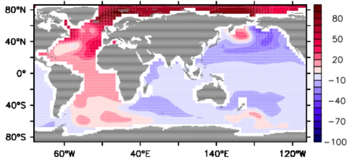
As an alternative to the attempt of identifying more or less complex spatial patterns of sea-level change, which are related to the AMOC strength, it is worth considering a simple large scale north–south gradient of sea-level rise. Levermann et al. (2005) have found such a distinct gradient in response to a freshwater-induced shutdown of the AMOC in idealized model simulations (Fig. 1). A similar pattern was also observed in the model average of SSH changes in the CMIP3 warming scenarios of the IPCC-AR4 (Meehl et al., 2007). This sea surface height anomaly η must be
Fig. 1.Equilibrium dynamic sea level change (in cm) after fresh-water induced collapse of the AMOC (800 yr of forcing as in Levermann et al., 2005).
approximately related via geostrophy to anomaliesuof zonal surface velocities:
f u= − 1
ρ0 ∂p ∂y ≈ −g
∂η
∂y, (1)
wheref is the Coriolis parameter. Only the upper branch of the MOC (in contrast to the currents contributing to the Gyres) crosses the Atlantic without a surface return flow: once from east to west in the South Atlantic, and then in the opposite direction mainly as the North Atlantic Current (NAC). Therefore, we expect a broad meridional SSH gradi-ent to correspond at least to the surface velocities belonging to the AMOC. The idea of a correspondence with depth inte-grated transport has been further pursued by Lorbacher et al. (2010). In agreement with Levermann et al. (2005), they in-deed find that a freshwater induced weakening of the AMOC is well correlated to a broad SSH rise in the NA relative to the South. While this is an encouraging result, it remains open if it also holds for AMOC changes induced by higher CO2
con-centrations under climate change or by remote forcing as in case of Southern Ocean winds. Also, Lorbacher et al. (2010) take into account only a single simulation and thus a single forcing strength. Therefore, it is also necessary to find out whether the linear relation is valid – and numerically iden-tical – for a sufficiently large parameter range. All of this must be fulfilled in order to use such a relation for diagnos-ing AMOC changes.
After a description of the model and the simulations in Sect. 2, we first compare (transient) sea-level patterns result-ing from three different forcresult-ing types in Sect. 3. Followresult-ing this, we present and analyze relations between the SL gradi-ent and AMOC changes based on simulations covering CO2,
2 Model simulations
All simulations have been performed with the Earth System Model of Intermediate Complexity CLIMBER-3α(Montoya et al., 2005) which is based on the ocean model MOM-3 (Pacanowski and Griffies, 1999) and a statistical-dynamical atmosphere (Petoukhov et al., 2000). The ocean module has a non-eddying horizontal resolution of 3.75◦ and a
verti-cal resolution of 24 layers, which together with the sim-plified atmosphere renders the model computationally ef-ficient for the relevant ensemble studies. Vertical mixing in the boundary layer is parameterized via the kpp-scheme (Large et al., 1994). The background values are 0.3 cm2s−1
for vertical diffusivity and 10 cm2s−1for vertical viscosity.
Isoneutral mixing is accomplished via Redi diffusion (Redi, 1982) with a diffusivity of 2.0×107cm2s−1 and
Gent-McWilliams eddy stirring (Gent and Gent-McWilliams, 1990) with 0.25×107cm2s−1. A nonlinear explicit free surface
formu-lation is used so that sea level is a prognostic variable and does not need to be diagnosed.
For our analysis of the relation between sea surface height and the AMOC, we focus on changes caused by freshwater fluxes into the northern convection sites, increases of CO2
concentration as well as modifications of Southern Ocean wind stress. All three forcings are known to determine the AMOC strength (Kuhlbrodt et al., 2007). The first two are ad-ditionally motivated by climate change since greenhouse gas concentrations have been rising and higher temperatures re-sult in larger meltwater runoff from the Greenland ice sheet. The Southern Ocean wind changes are a remote forcing quite different from the others, and it may indicate if a relation between AMOC and SL is universal or just consists of two separate reactions to local buoyancy forcing. However, it is not certain in how far the response of the Southern Ocean to this forcing would be different in eddy-permitting simula-tions, because energetic eddies might partly compensate the reaction of the Ekman transport (e.g. Farneti and Delworth, 2010; Farneti et al., 2010; Spence et al., 2010).
If not otherwise mentioned, all simulations are started from an equilibrium state under preindustrial conditions (CO2 concentration of 280 ppm), and forcing strengths are
linearly increased within 100 yr from zero to a value which we will in the following calltarget value. Freshwater forc-ing has been applied as a negative salt flux in the region be-tween 52◦N and 80◦N as well as 48◦W and 15◦E, excluding
shallow areas over the continental shelves (same forcing area as in Fig. 1). The flux has been compensated in the Pacific ocean. The Southern Ocean wind stress anomalies have been applied south of 31.875◦S. As our emphasis is on better
un-derstanding the principle relations underlying the three forc-ings, we exclude feedbacks involving wind stress by keeping it fixed at its climatological values unless modified explic-itly. Since we exclusively focus on relative regional sea level rise, changes in global sea level have been subtracted for all model results in the paper.
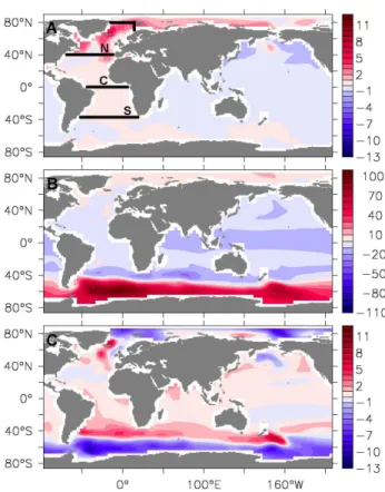
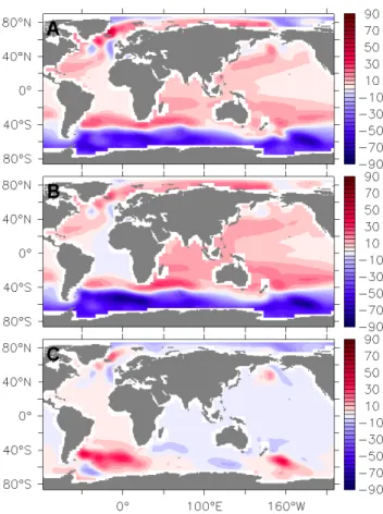
Fig. 2.Dynamic sea level rise in cm Sv−1 (i.e. normalized to a
weakening of the AMOC by 1 Sv), after 100 yr of the following forcings:(A)freshwater with a target value of 0.064 Sv,(B) South-ern Ocean winds approaching zero,(C)CO2with a target
concen-tration of 500 ppm.
3 SSH patterns resulting from the three different forcings
We first compare the sea-level anomalies resulting from 100 yr of simulation under the three different types of forc-ing and several different strengths. The patterns have been divided by the amount of AMOC reduction induced by this forcing for normalization (Fig. 2). The target value of the applied freshwater forcing is 0.064 Sv leading to an AMOC weakening of 2.0 Sv. In order to get a sufficiently strong reduction of the AMOC after these first 100 yr, we let the Southern Ocean wind stress approach zero, which results in a change of the AMOC streamfunction maximum by
−1.24 Sv. The final CO2concentration amounts to 500 ppm
concomitant with an AMOC weakening of 2.0 Sv as in the case of freshwater forcing.
In case of freshwater forcing (top panel), the most promi-nent pattern is a rise of sea level in the Atlantic north of 40◦
on sea level are transmitted to more distant regions, e.g. the South Atlantic.
A reduction of the Southern Ocean wind stress (middle panel) also results primarily in a localized sea level reac-tion. The surface currents in the ACC region are directly slowed down and sea level south of the ACC rises as expected from geostrophy. However, the SL difference in the Atlantic section of the Southern Ocean is not linearly linked to the AMOC when the latter increases and decreases in strength due to modifications of the wind stress (not shown).
The overturning strength is of course not in equilibrium after these first 100 yr. In year 500, from when onwards the AMOC maximum remains rather constant (or oscillates around a quite stable value), the sea-level response turns out to be less localized with a reaction in the North Atlantic for the wind stress forcing, and a reaction in the Southern Ocean in the case of freshwater forcing.
In case of rising CO2concentration (bottom panel), we
ap-ply a global forcing and indeed significant adaptations of sea level height are induced in multiple regions. The most promi-nent features are a relative rise of sea level in the convection areas of the North Atlantic as well as a drop of sea level in the Weddell Gyre and to a lesser extent in further domains south of the ACC.
Comparing these three figures, we can not identify a com-mon sea-level pattern, which could directly correspond to a change of the AMOC maximum independently of the forcing type. However, Fig. 2 supports the link between a system-atic north–south SL gradient in the Atlantic and the AMOC which has been discussed above. In the following section, we will thus analyze the relation of AMOC changes and SL differences between three parts of a subdivided Atlantic Ocean: (N)orth, (C)entral and (S)outh, bounded by the 80◦
-latitude, the 41.25◦-latitude, the equator and the tip of South
Africa as indicated in the top panel of Fig. 2. We focus on the averages of these broad boxes as we aim at robust results that are less dependent on potentially model-specific localized SL reactions.
4 Relation of an Atlantic north–south disparity in SSH to the AMOC
4.1 100 yr of forcing
For a total of 100 yr and for a variety of forcing strengths, we present the relations of AMOC maximum and differences in sea-level change between (N) and (C) as well as (N) and (S). The target values of freshwater forcing (cf. Sect. 2) are var-ied between 0.06 Sv and 0.2 Sv, the strength of the Southern Ocean wind stress by factors 0 to 4.0; the target values of CO2 concentration range from 350 ppm to 1120 ppm. Two
simulations with exponential increase of CO2concentration
(0.5 % and 1.0 % per year) are additionally included.
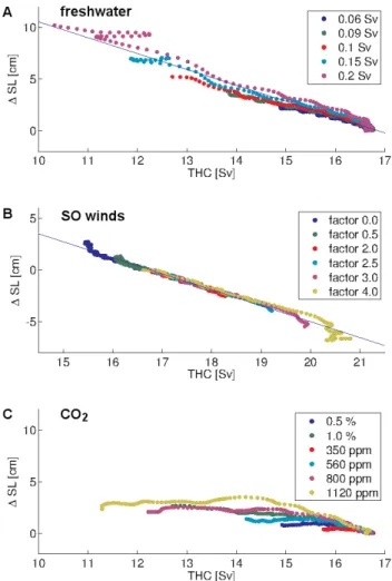
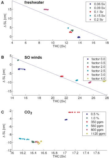
Fig. 3.1SL between North and Central for the following forcings: (A)freshwater (slope:−1.53 cm Sv−1),(B)Southern Ocean winds
(slope:−1.54 cm Sv−1),(C)CO 2.
Plotted against the AMOC strength, Fig. 3 shows the dif-ference in average sea level rise of the northern and the central part, and Fig. 4 between the northern and southern part. These two plots are quite similar, reflecting the fact that most significant relative displacements of SSH occur north of the equator, especially around the latitude of 40◦. The main
difference is the stronger reduction of1SLNScompared to 1SLNCfor CO2forcing in the second half of the simulated
timespan. Below, we will specifically comment on the pecu-liarities of thermal forcing (see Sect. 4.3); but for now, this motivates us to choose the difference between northern and central area as a representative of the SL rise gradient.
For the difference in sea-level change between these two areas in response to freshwater and wind stress forcing, each of the top and middle panels of Fig. 3 also shows an objec-tive linear least square fit giving a slope of−1.53 cm Sv−1
and−1.54 cm Sv−1, respectively. These relations are
Fig. 4.1SL between North and South for the following forcings: (A)freshwater (slope:−1.57 cm Sv−1),(B)Southern Ocean winds
(slope:−0.94 cm Sv−1),(C)CO 2.
appears consistent with the map of dynamic sea-level change per Sverdrup of AMOC reduction given by Lorbacher et al. (2010) and presented in their Fig. 8a. However, increases of CO2 concentration lead to more non-linear relations when
time progresses. This makes it essentially impossible to diag-nose an AMOC change from relative SL rise in this manner. But note that the initial slope of the stronger forcings is quite similar to the one originating from the first two forcing types, which may be an indicator for an initially universal behavior. In a different setting of almost no vertical diffusivity and for equilibrium states, Griesel and Maqueda (2006) ana-lyze among other aspects the relation between AMOC and sea surface height when the density structure of the ocean is modified. This modification is done especially by alter-ing Gent-McWilliams coefficients, but also by surface forc-ings including freshwater and wind as well as an increase in vertical diffusivity. Having a different objective, we look at the transient behavior and all of our forcings are com-bined with a realistic rather than almost zero vertical diffu-sivity, while considering different forcings with a range of
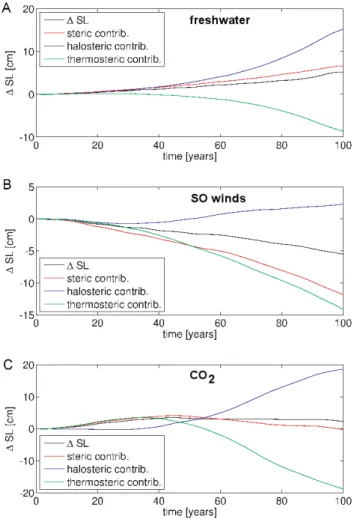
Fig. 5.1SL between North and Central and the contributions due to steric SLR as well as a subdivision into halosteric and thermosteric SLR:(A)freshwater forcing (0.1 Sv),(B)Southern Ocean winds (factor 3.0),(C)linear increase of CO2to 1120 ppm.
strengths. However, some further universality of our above relations for freshwater and wind forcing is indicated by the quite similar linear relation between SSH difference ([40◦
to 60◦N] minus [20◦ to 30◦N], at a longitude of 44◦W)
and AMOC with a slope of about−2 cm Sv−1observed by
Griesel and Maqueda (2006).
While we have also analyzed the consequences of includ-ing all latitudes from Antarctica to the North Pole and sec-tioning this extended Atlantic (not shown), the inclusion of the Southern Ocean does not produce the apparently robust linear relations seen in Fig. 3a and b, because the positive and negative changes around the ACC do not balance out and thus interfere with the relation found in the Atlantic further north.
halosteric effect dominates in the freshwater case and the thermosteric effect dominates in case of modified Southern Ocean winds. The significant role of mass redistribution (the difference between total SL change and the steric contribu-tion) is remarkable.
4.2 Longer timescale
For checking in how far the relations are dependent on the continuous increase of the forcing and on the relatively short timescale of 100 yr, we did two further analyses. Firstly, we have included the evolution of AMOC and SL for another 100 yr in which we keep the forcing constant at its target value. Secondly, we have performed a set of experiments in which also 200 yr of data are included but now with a slower increase of the forcing so that the target value is only reached at the end of this 200-yr period.
Including the additional 100 yr of the first case, the re-sults deviate significantly from the original ones and nei-ther of the two approximately linear relations is confirmed for this time period. The same is valid for the second set of 200-yr experiments, although the deviations are smaller. This illustrates the limitations of the transient relations. At this point, the tracer redistribution seems to lead to a state in which the vertical structure of density changes has suf-ficient time to change so that the relation between changes in depth-integrated transport and sea level is modified. It is noticeable that the linear relation breaks down for especially strong AMOC changes in Sect. 4.1. However, during the sec-ond century (at least in some of the simulations) no further reduction of the AMOC strength goes along with the break-down of the linear relation. This indicates that the cause for the breakdown is not the amount of the AMOC change itself but the strength of the forcing combined with its timescale.
One may now wonder if the system approaches an equi-librium on a longer timescale when a linear relation between AMOC and sea level might be reestablished. Therefore, we have extended the original runs with constant forcing up to the year 1000. Figure 6 covers the last 10 yr of the simula-tion, also illustrating the changes still occurring at this point of time. The slopes found in Sect. 4.1 are plotted into Fig. 6 for reference.
In case of freshwater forcing, the data is still scattered along a linear relation but with roughly double the slope and a different offset. This shows that with the continuous accu-mulation of freshwater, the impact on the sea level difference between north and center gets larger while the AMOC only weakens relatively little after the first 100 yr. For modified Southern Ocean wind stress, the situation is quite the oppo-site. When the wind stress is held constant after an increase, the AMOC continues to intensify and reaches maxima that are significantly larger after 1000 yr. The consequence is a linear best fit with a smaller slope. However, a significantly stronger weakening of the AMOC cannot be achieved via a weakening of the Southern Ocean winds even on this long
Fig. 6.1SLNCafter 1000 yr for the following forcings:(A)
fresh-water,(B)Southern Ocean winds,(C)CO2. The lines in the upper two panels follow Fig. 3.
timescale and the linear fit is not as good as in the freshwa-ter forcing case. For both types of simulations, the vertical profile of density changes gets modified in the longer run compared to the first 100 yr. This means that a preexisting specific linear relation between changes in the sea-level dif-ferences and in the depth-integrated pressure difdif-ferences will degrade, no matter if there is a continuous linear scaling be-tween the latter and the AMOC or not.
It was suggested a long time ago that the AMOC strength recovers approximately to its original value when an equilib-rium state with higher CO2concentration is reached: Manabe
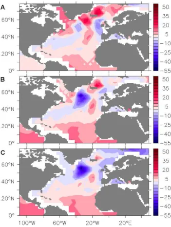
Fig. 7.Sea-level anomaly (zero global mean) in cm for linearly in-creasing CO2 concentration (to 1120 ppm within 100 yr) at three
different times:(A)year 100,(B)year 500,(C)year 1000.
discussed in the following subsection, we note that none of the relations described in the previous subsection is retained on the thousand year timescale.
4.3 Special role of CO2forcing
The initial weakening followed by a recovery of the AMOC in case of CO2forcing is easily understood: While as a first
reaction the heat exchange in the deepwater-formation gions is reduced, instabilities of the water column can re-occur when the deeper ocean layers also have adjusted to the warmer climate. However, instead of vanishing when the AMOC is stabilized roughly at its original value, relative SLR is larger south of 30◦N than north of 30◦N. This is also
reflected by the negative1SL in the lower panel of Fig. 6. Time slices of sea-level anomaly patterns in the North At-lantic (Fig. 7) illustrate this effect for a linear increase of CO2
concentration to 1120 ppm within 100 yr (concentration kept constant thereafter).
Fig. 8. (A)AMOC maximum, and(B) sea-level anomaly at the North American coast (zero global mean). CO2concentration is
lin-early increased to 1120 ppm within the first 100 yr.
Looking at the more local development, Fig. 8 shows a time series of the AMOC maximum and the average sea level of a fraction of the North American coast: between 41◦N (1◦
north of New York City) and 60◦N. While the AMOC
sta-bilizes, the transient SLR at the American coast is overcom-pensated, reaching a negative value rather than returning to the original equilibrium state.
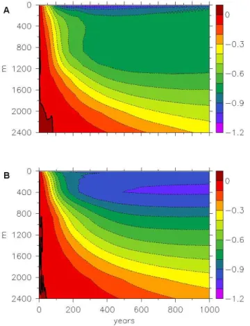
Fig. 9.Potential density anomaly (kg m−3) for linearly
increas-ing CO2concentration (to 1120 ppm within 100 yr): (A)average of northern area,(B)average of central area.
in the top 200 m warms more strongly in the north, but den-sity is reduced more strongly in the south because of the temperature dependence of the equation of state. However, the striking thermal expansion in the south centered around 400 m depth is due directly to stronger warming.
4.4 Combined forcings based on RCP scenarios
After this highly idealized study of fully independent forc-ing types, let us now turn to somewhat more realistic scenar-ios. The initial condition of the following simulations is pro-duced by an integration over the time period between 1767 and 2005 on the basis of RCP historical forcing data (Mein-shausen et al., 2011b). For the years 2006 to 2100, we have simulated all 4 RCP scenarios and an additional set of ex-periments in which we have also included high estimates of idealized Greenland freshwater forcing with target values of 0.042 to 0.13 Sv. The RCP forcing as applied by us consists of greenhouse gases, direct effects of sulphate aerosols, land-use change and solar variability. For the historic forcing lead-ing to the initial condition, volcanic forclead-ing was also taken into account.
Fig. 10.1SLNCfor 100 yr relative to 2005 for the following
forc-ings:(A)4 RCP-scenarios,(B)RCP-scenarios plus freshwater forc-ing (slope of linear fit:−0.50 cm Sv−1).
Changes in the hydrological cycle are automatically re-flected in the simulations. However, the freshwater flux due to meltwater runoff from Greenland has to be separately es-timated. As its magnitude is highly uncertain, we have based our study on a best guess with the aim to see how parallel application of CO2and freshwater forcing behave in
princi-ple. As in the preceding subsections, we linearly increase the freshwater flux from 0 to its target value between the years 2006 and 2100, and we apply it to the same area as in the preceding subsections, not taking into account regional dis-tributions due to the Greenland boundary currents.
For no future temperature change, we assume a constant current Greenland mass loss rate of 250 Gt yr−1 (Rignot
et al., 2011) which corresponds to about 7 cm SLR until 2100. Motivated by the results of Pfeffer et al. (2008), we choose an accumulated mass loss of 54 cm until the year 2100 for the strongest scenario (RCP8.5). Linearly scal-ing the freshwater fluxes between these two values for the other scenarios on the basis of the median global temper-atures reached in the year 2100 as calculated with MAG-ICC6 (Meinshausen et al., 2011a), we apply target values of 0.042 Sv, 0.066 Sv, 0.085 Sv and 0.13 Sv for the scenar-ios RCP3-PD, RCP4.5, RCP6 and RCP8.5 respectively. We then keep the fluxes fixed for another five years in order to compare a total of 100 yr with the results of Sect. 4.1.
The results with and without freshwater forcing are pre-sented in Fig. 10. The pure RCP-forcing scenarios provide a picture qualitatively similar to the case of idealized CO2
sea-level difference as well as with respect to the shapes of the curves. When combining both forcings, we do see lin-ear trends for the largest fraction of the 100 yr. However, the slopes are smaller than in case of pure freshwater forcing and they are significantly different between the scenarios. The large drop of the SLR difference in the last 30 yr of the simu-lation with strongest forcing goes along with a strongly non-linear strengthening of the Subpolar Gyre in our model (Lev-ermann and Born, 2007). The results in Fig. 10 confirm that the approach as it is cannot be used for diagnosing a weaken-ing of the AMOC under climate change, not even under the assumption of strong and fixed Greenland runoff going along with each of the RCP scenarios.
5 Additivity of SSH patterns and AMOC strengths
In the preceding section, we have shown relations between AMOC strength and an Atlantic sea level difference for three types of forcing, but they turned out to be unsuitable as an AMOC diagnostic. Possibly other models, preferably with a higher resolution, may reveal more fine-structured patterns of which each corresponds to AMOC changes under a spe-cific forcing and which are likely different from each other (cf. Fig. 2). In that case, it would be essential that the AMOC changes belonging to the individual forcings as well as the corresponding patterns of sea-level change add up linearly. If this were true, one might be able to deduce the contribut-ing patterns as well as the contributcontribut-ing and total AMOC re-ductions from the observed sea-level changes (which are in general caused by the simultaneous action of different forc-ings). However, already the case of RCP scenarios with ad-ditional meltwater fluxes in the previous section reveals that the AMOC reductions do not add up linearly. We examine this aspect further in this section.
5.1 Additivity of SSH patterns
We do not attempt a quantitative analysis of the linear regime for the different parameters. Instead, we aim at illustrating that the large-scale patterns of sea-level change simulated by our model can be superposed reasonably well for our exam-ple forcings.
We choose the case of CO2increase by 1 % per year,
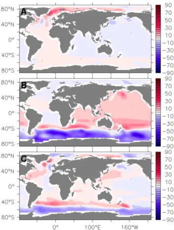
dou-bling of the Southern Ocean winds within 100 yr and a fresh-water flux with a target value of 0.09 Sv. The sum of the sea-level anomalies after the first 100 yr is compared with the pat-tern resulting from the application of all three types of forc-ing at the same time. In contrast to the simulations in the pre-ceding two sections where we were interested in the isolated effects of specific forcings, we now have included the wind stress feedback instead of keeping the wind stress fixed at its climatological values. Figure 11 shows the patterns of the three individual forcings, while Fig. 12 shows the sum of the patterns, the pattern resulting from the application of all three
Fig. 11.Sea-level anomaly (cm) for individual forcings after 100 yr: (A)freshwater,(B)SO winds,(C)CO2.
forcings and the difference between the two. Qualitatively, the patterns can be linearly superposed on a large scale. How-ever, the regions of more pronounced non-linearity are those with a strong signal: the northern convection sites, the subpo-lar gyres and the ACC. This already influences the sea-level difference between the two areas (N) and (C) that we have discussed above.
5.2 Additivity of AMOC weakening
For checking the additivity of the individual changes in AMOC strength, we have applied the same forcings as in the preceding subsection. Figure 13 shows a time series of the first 200 yr. While the sum of the individual AMOC changes coincides very well with the anomaly due to combined forc-ing for the first 80 yr and a total AMOC change of about 4 Sv, we observe that they differ significantly thereafter.
This suggests that the range of applicability of a hypotheti-cal AMOC diagnostic involving different SL change patterns for different forcings is limited.
Fig. 12. (A)Sum of the three anomalous sea-level fields given in Fig. 11,(B)sea-level anomaly resulting from application of all three forcings,(C)difference of the fields in(A)and(B).
the same magnitude of freshwater-forcing if the wind-stress feedback is disabled, it does occur even without variable wind stress when applying some other forcing strengths.
6 Conclusions
We were aiming at identifying a robust transient relation between a gradient of sea-level change in the Atlantic and changes of the AMOC on the basis of an ensemble study with a coarse resolution model that parameterizes eddy fluxes. We did indeed find a linear relation for Southern Ocean wind and freshwater forcing, which has a slope of about−1.5 cm Sv−1
with respect to the difference in sea-level change between two areas in the North Atlantic. While a somewhat similar slope was found for an initial short period of strong changes in CO2 concentration, this relation does not hold for the
largest fraction of the simulations and is also dependent on the forcing strength. For each of the less idealized settings of four RCP scenarios with associated freshwater forcing mo-tivated by Greenland meltwater runoff, transient linear rela-tions of the SL difference and AMOC weakening are mainly confirmed. However, the slopes quantitatively differ between the different scenarios. Because of the great relevance of CO2
0 50 100 150 200
-10 -8 -6 -4 -2 0 2
Time [a]
∆
AMOC [Sv] Freshwater SO winds Carbon dioxide Sum
Combined forcing
Fig. 13.AMOC changes for individual forcings and for combined forcing.
forcing, these results exclude using the sea-level difference or gradient as a direct AMOC diagnostic under climate change. It is therefore desirable to focus on the analysis of more detailed patterns of sea-level change, which might lead to fingerprints for different forcing mechanisms similar to the sea-level patterns provided in Sect. 3. However, for such a study, more complex models based on a higher resolution are likely to be better suited. We demonstrated in a short outlook that individual large-scale patterns of SSH change as well as AMOC changes can be linearly superposed reasonably well for the given forcing strengths in a limited timeframe of 80 yr (Figs. 12 and 13). Thus, if different relations for different forcing types are found in the future, they might be able to serve as an AMOC diagnostic under the realistic simultane-ous action of several forcings; but the indicated limitations regarding additivity would have to be further explored.
Acknowledgements. We thank Georg Feulner and Till Kuhlbrodt
for helpful discussions and we are grateful to the anonymous referees for their comments. H. K. acknowledges support by the Evangelisches Studienwerk Villigst e.V. and the German National Academic Foundation.
Edited by: K. Keller
References
Broecker, W. S.: Unpleasant surprises in the greenhouse?, Nature, 328, 123–126, 1987.
Bryan, F.: Parameter sensitivity of primitive equation ocean general circulation models, J. Phys. Oceanogr., 17, 970–985, 1987. de Boer, A. M., Gnanadesikan, A., Edwards, N. R., and Watson,
A. J.: Meridional density gradients do not control the Atlantic overturning circulation, J. Phys. Oceanogr., 40, 368–380, 2010. Dohan, K. and Maximenko, N.: Monitoring ocean currents with
satellite sensors, Oceanography, 23, 94–103, 2010.
Farneti, R., Delworth, T. L., Rosati, A. J., Griffies, S. M., and Zeng, F.: The role of mesoscale eddies in the rectification of the South-ern Ocean response to climate change, J. Phys. Oceanogr., 40, 1539–1557, 2010.
Gent, P. R. and McWilliams, J. C.: Isopycnal mixing in ocean cir-culation models, J. Phys. Oceanogr., 20, 150–155, 1990. Gnanadesikan, A.: A simple predictive model for the structure of
the oceanic pycnocline, Science, 283, 2077–2079, 1999. Gregory, J. M., Dixon, K. W., Stouffer, R. J., Weaver, A. J.,
Driess-chaert, E., Eby, M., Fichefet, T., Hasumi, H., Hu, A., Jung-claus, J. H., Kamenkovich, I. V., Levermann, A., Montoya, M., Murakami, S., Nawrath, S., Oka, A., Sokolov, A. P., and Thorpe, R. B.: A model intercomparison of changes in the At-lantic thermohaline circulation in response to increasing atmo-spheric CO2 concentration, Geophys. Res. Lett., 32, L12703,
doi:10.1029/2005GL023209, 2005.
Griesel, A. and Morales Maqueda, M. A.: The relation of meridional pressure gradients to North Atlantic deep water volume transport in an ocean general circulation model, Clim. Dynam., 26, 781– 799, 2006.
H¨akkinen, S.: Variability in sea surface height: A qualitative mea-sure for the meridional overturning in the North Atlantic, J. Geo-phys. Res.-Oceans, 106, 13837–13848, 2001.
Hofmann, M. and Rahmstorf, S.: On the stability of the Atlantic meridional overturning circulation, P. Natl. Acad. Sci., 106, 20584–20589, 2009.
Hu, A. X., Meehl, G. A., and Han, W. Q.: Detecting thermohaline circulation changes from ocean properties in a coupled model, Geophys. Res. Lett., 31, L13204, doi:10.1029/2004GL020218, 2004.
Hughes, T. M. C. and Weaver, A. J.: Multiple equilibria of an asym-metric 2-basin ocean model, J. Phys. Oceanogr., 24, 619–637, 1994.
Ivchenko, V. O., Sidorenko, D., Danilov, S., Losch, M., and Schr¨oter, J.: Can sea surface height be used to estimate oceanic transport variability?, Geophys. Res. Lett., 38, L11601, doi:10.1029/2011GL047387, 2011.
Kanzow, T., Hirschi, J. J. M., Meinen, C., Rayner, D., Cunningham, S. A., Marotzke, J., Johns, W. E., Bryden, H. L., Beal, L. M., and Baringer, M. O.: A prototype system for observing the Atlantic meridional overturning circulation – scientific basis, measure-ment and risk mitigation strategies, and first results, J. Operat. Oceanogr., 1, 19–28, 2008.
K¨orper, J., Spangehl, T., Cubasch, U., and Huebener, H.: Decom-position of projected regional sea level rise in the north Atlantic and its relation to the AMOC, Geophys. Res. Lett., 36, L19714, doi:10.1029/2009GL039757, 2009.
Kuhlbrodt, T., Griesel, A., Montoya, M., Levermann, A., Hofmann, M., and Rahmstorf, S.: On the driving processes of the Atlantic meridional overturning circulation, Rev. Geophys., 45, RG2001, doi:10.1029/2004RG000166, 2007.
Landerer, F. W., Jungclaus, J. H., and Marotzke, J.: Regional dy-namic and steric sea level change in response to the IPCC-A1B scenario, J. Phys. Oceanogr., 37, 296–312, 2007.
Large, W. G., McWilliams, J. C., and Doney, S. C.: Oceanic vertical mixing: A review and a model with a nonlocal boundary layer parameterization, Rev. Geophys., 32, 363–403, 1994.
Latif, M., Roeckner, E., Botzet, M., Esch, M., Haak, H., Hage-mann, S., Jungclaus, J., Legutke, S., Marsland, S., Mikolajewicz,
U., and Mitchell, J.: Reconstructing, monitoring, and predicting multidecadal-scale changes in the North Atlantic thermohaline circulation with sea surface temperature, J. Climate, 17, 1605– 1614, 2004.
Latif, M., Boning, C., Willebrand, J., Biastoch, A., Dengg, J., Keenlyside, N., Schweckendiek, U., and Madec, G.: Is the thermohaline circulation changing?, J. Climate, 19, 4631–4637, 2006.
Lee, T., H¨akkinen, S., Kelly, K., Qiu, B., Bonekamp, H., and Lind-strom, E. J.: Satellite observations of ocean circulation changes associated with climate variability, Oceanography, 23, 70–81, 2010.
Levermann, A. and Born, A.: Bistability of the Atlantic subpolar gyre in a coarse-resolution climate model, Geophys. Res. Lett., 34, L24605, doi:10.1029/2007GL031732, 2007.
Levermann, A., Griesel, A., Hofmann, M., Montoya, M., and Rahmstorf, S.: Dynamic sea level changes following changes in the thermohaline circulation, Clim. Dynam., 24, 347–354, 2005. Levermann, A., Mignot, J., Nawrath, S., and Rahmstorf, S.: The role of northern sea ice cover for the weakening of the thermo-haline circulation under global warming, J. Climate, 20, 4160– 4171, 2007.
Lorbacher, K., Dengg, J., B¨oning, C. W., and Biastoch, A.: Regional patterns of sea level change related to interannual variability and multidecadal trends in the Atlantic meridional overturning circu-lation, J. Climate, 23, 4243–4254, 2010.
Manabe, S. and Bryan Jr., K.: CO2-Induced change in a coupled
Ocean-Atmosphere model and its paleoclimatic implications, J. Geophys. Res., 90, 11689–11707, 1985.
Manabe, S. and Stouffer, R. J.: Century-scale effects of increased atmospheric C02on the ocean-atmosphere system, Nature, 364,
215–218, 1993.
Meehl, G. A., Stocker, T. F., Collins, W. D., Friedlingstein, P., Gaye, A. T., Gregory, J. M., Kitoh, A., Knutti, R., Murphy, J. M., Noda, A., Raper, S. C. B., Watterson, I. G., Weaver, A. J., and Zhao, Z.-C.: Climate Change 2007: The Physical Science Basis, Contribu-tion of Working Group I to the Fourth Assessment Report of the Intergovernmental Panel on Climate Change, Chap. Global Cli-mate Projections, Cambridge University Press, Cambridge, UK and New York, NY, USA, 2007.
Meinshausen, M., Wigley, T. M. L., and Raper, S. C. B.: Emulat-ing atmosphere-ocean and carbon cycle models with a simpler model, MAGICC6 – Part 2: Applications, Atmos. Chem. Phys., 11, 1457-1471, doi:10.5194/acp-11-1457-2011, 2011a. Meinshausen, M., Smith, S. J., Calvin, K., Daniel, J. S., Kainuma,
M. L. T., Lamarque, J.-F., Matsumoto, K., Montzka, S. A., Raper, S. C. B., Riahi, K., Thomson, A., Velders, G. J. M., and van Vu-uren, D. P. P.: The RCP greenhouse gas concentrations and their extensions from 1765 to 2300, Climatic Change, 109, 213–241, 2011b.
Montoya, M., Griesel, A., Levermann, A., Mignot, J., Hofmann, M., Ganopolski, A., and Rahmstorf, S.: The earth system model of intermediate complexity CLIMBER-3α, Part 1: description and performance for present-day conditions, Clim. Dynam., 25, 237– 263, 2005.
Petoukhov, V., Ganopolski, A., Brovkin, V., Claussen, M., Eliseev, A., Kubatzki, C., and Rahmstorf, S.: CLIMBER-2: a climate sys-tem model of intermediate complexity, Part I: model description and performance for present climate, Clim. Dynam., 16, 1–17, 2000.
Pfeffer, W. T., Harper, J. T., and O’Neel, S.: Kinematic constraints on glacier contributions to 21st-Century Sea-Level rise, Science, 321, 1340–1343, 2008.
Redi, M. H.: Oceanic isopycnal mixing by coordinate rotation, J. Phys. Oceanogr., 12, 1154–1158, 1982.
Rignot, E., Velicogna, I., van den Broeke, M. R., Monaghan, A., and Lenaerts, J.: Acceleration of the contribution of the Greenland and Antarctic ice sheets to sea level rise, Geophys. Res. Lett., 38, L05503, doi:10.1029/2011GL046583, 2011.
Spence, Pa., Fyfe, J. C., Montenegro, A., and Weaver, A. J.: Southern Ocean Response to Strengthening Winds in an Eddy-Permitting Global Climate Model, J. Climate, 23, 5332–5343, 2010.
Stommel, H.: Thermohaline convection with 2 stable regimes of flow, Tellus, 13, 224–230, 1961.
Thorpe, R. B., Gregory, J. M., Johns, T. C., Wood, R. A., and Mitchell, J. F. B.: Mechanisms determining the Atlantic thermo-haline circulation response to greenhouse gas forcing in a non-flux-adjusted coupled climate model, J. Climate, 14, 3102–3116, 2001.
Willis, J. K.: Can in situ floats and satellite altimeters detect long-term changes in Atlantic ocean overturning?, Geophys. Res. Lett., 37, L06602, doi:10.1029/2010GL042372, 2010.
