Sea level trend and variability around the Peninsular Malaysia

(1)

OSD

11, 1519–1541, 2014

Sea level trend and variability around the

Peninsular Malaysia

Q. H. Luu et al.

Title Page

Abstract Introduction

Conclusions References

Tables Figures

◭ ◮

Back Close

Full Screen / Esc

Printer-friendly Version Interactive Discussion

Discussion

P

a

per

|

Discus

sion

P

a

per

|

Discussion

P

a

per

|

Discussion

P

a

per

|

Ocean Sci. Discuss., 11, 1519–1541, 2014 www.ocean-sci-discuss.net/11/1519/2014/ doi:10.5194/osd-11-1519-2014

This discussion paper is/has been under review for the journal Ocean Science (OS). Please refer to the corresponding final paper in OS if available.

Sea level trend and variability around the

Peninsular Malaysia

Q. H. Luu, P. Tkalich, and T. W. Tay

Tropical Marine Science Institute, National University of Singapore, Singapore

Received: 16 April 2014 – Accepted: 15 May 2014 – Published: 17 June 2014

Correspondence to: Q. H. Luu (tmslqh@nus.edu.sg)

(2)

OSD

11, 1519–1541, 2014

Q. H. Luu et al.

Title Page

Tables Figures

◭ ◮

Back Close

Full Screen / Esc

Discussion

P

a

per

|

Discus

sion

P

a

per

|

Discussion

P

a

per

|

Discussion

P

a

per

|

Abstract

Peninsular Malaysia is bounded from the west by Malacca Strait and the Andaman Sea both connected to the Indian Ocean, and from the east by South China Sea being largest marginal sea in the Pacific Basin. Resulting sea level along Peninsu-lar Malaysia coast is assumed to be governed by various regional phenomena as-5

sociated with the adjacent parts of the Indian and Pacific Oceans. At annual scale, sea level anomalies (SLAs) are generated by the Asian monsoon; interannual sea level variability is determined by the El Niño–Southern Oscillation (ENSO) and the Indian Ocean Dipole (IOD); while long-term sea level trend is related to global cli-mate change. To quantify the relative impacts of these multi-scale phenomena on 10

sea level trend and variability around the Peninsular Malaysia, long-term tide gauge record and satellite altimetry are used. During 1984–2011, relative sea level rise (SLR) rates in waters of Malacca Strait and eastern Peninsular Malaysia are found to be 2.4±1.6 mm yr−1and 2.7±1.0 mm yr−1, respectively. Allowing for corresponding

verti-cal land movements (VLM; 0.8±2.6 mm yr−1and 0.9±2.2 mm yr−1), their absolute SLR 15

rates are 3.2±4.2 mm yr−1and 3.6±3.2 mm yr−1, respectively. For the common period

1993–2009, absolute SLR rates obtained from both tide gauge and satellite altimetry in Peninsular Malaysia are similar; and they are slightly higher than the global tendency. It further underlines that VLM should be taken into account to get better estimates of SLR

observations. At interannual scale, ENSO affects sea level over the Malaysian coast in

20

the range of±5 cm with a very high correlation. Meanwhile, IOD modulates sea level

anomalies mainly in the Malacca Strait in the range of ±2 cm with a high correlation

coefficient. Interannual regional sea level drops are associated with El Niño events and positive phases of the IOD index; while the rises are correlated with La Niña episodes and the negative periods of the IOD index. Seasonally, SLAs are mainly monsoon-25

(3)

OSD

11, 1519–1541, 2014

Q. H. Luu et al.

Title Page

Tables Figures

◭ ◮

Back Close

Full Screen / Esc

Discussion

P

a

per

|

Discus

sion

P

a

per

|

Discussion

P

a

per

|

Discussion

P

a

per

|

of Peninsular Malaysia, mostly due to East Asian-Western Pacific Monsoon. These results imply that a narrow topographic constriction in Singapore Strait may separate different modes of annual and interannual sea level variability along coastline of Penin-sular Malaysia.

1 Introduction 5

The Peninsular Malaysia is located on the middle of Sunda Shelf, encompassed from the east by the South China Sea (SCS) being the largest marginal sea in the Pacific Basin, and from the west by the Andaman Sea of the Indian Ocean. Sea level around the Peninsular Malaysia is governed by a variety of phenomena, ranging from global to regional scales, resulting in complicated sea level trend and variability along the coast. 10

It is well established that global mean sea level (GMSL) has been rising at the rate

of 1.7±0.2 mm yr−1 since the beginning of last century (Nerem et al., 2006; Church

and White, 2011; Stammer et al., 2013). A significant acceleration of sea level rise

(SLR) in the order of 0.01 mm yr−2 has also been observed since early 20th century,

leading to the rate of 1.9±0.4 mm yr−1 during the 1961–2009 era (Jevrejeva, 2008;

15

Church and White, 2011). For the recent period (1993–2009), GMSL has been rising much faster: in situ data displayed the rate 2.8±0.8 mm yr−1(Church and White, 2011),

while satellite altimetry suggested a consistent increment of 3.3±0.4 mm yr−1(Nicholls

and Cazenave, 2010). However, sea level change is highly non-uniform spatially and temporally, mostly due to local adjustment to the global warming as well as variability 20

of regional climate drivers. For example, in the tropical western Pacific and eastern

Indian Oceans, rise rate seemingly approached 30 mm yr−1 for the period 1993–2001

(Church et al., 2006; Becker et al., 2012); however, this pattern was largely attributed to the variability of El Niño–Southern Oscillation (ENSO) and North Pacific Decadal Os-cillation (Trenberth and Hurrell, 1994; Church et al., 2004; Becket et al., 2012; Tkalich 25

(4)

OSD

11, 1519–1541, 2014

Q. H. Luu et al.

Title Page

Tables Figures

◭ ◮

Back Close

Full Screen / Esc

Discussion

P

a

per

|

Discus

sion

P

a

per

|

Discussion

P

a

per

|

Discussion

P

a

per

|

the adjacent region. Thus, quantification of regional sea level trend requires sufficiently long datasets to filter out the climate variability.

In areas adjacent to the Peninsular Malaysia, a few studies have analyzed sea level trends, including the Gulf of Thailand (Trisirisatayawong et al., 2011), the Sin-gapore Strait (Tkalich et al., 2013) and the SCS (Peng et al., 2013). Trisirisatayawong 5

et al. (2011) used tide gauge data corrected by the Vertical Land Motion (VLM) to ob-tain a SLR rate 3.0±1.5 mm yr−1for the Gulf of Thailand during the period 1940–2004,

thus qualifying the rate to be significantly faster than the global tendency. In the

Sin-gapore Strait, Tkalich et al. (2013) obtained a SLR rate of 1.2–1.7 mm yr−1 during the

period 1975–2009 and 1.8–2.4 mm yr−1 during the years 1984–2009. Taking into

ac-10

count an estimate of land subsidence rate, 1–1.5 mm yr−1

in Singapore, the trend of absolute SLR in the strait follows the regional tendency. Recently, Peng et al. (2013) examined the sea level trend and variability in the SCS since 1950 by analyzing two-dimensional past sea level reconstruction (produced by Meyssignac et al., 2012) and observed satellite altimetry. For the period 1993–2009, it was found that the recon-15

structed sea levels exhibit an average rise speed of 3.6±0.4 mm yr−1, which is

sim-ilar to the satellite altimetry rate of 3.9±0.9 mm yr−1. On average, the SLR rate over

1950–2009 period was estimated at 1.7±0.1 mm yr−1, which is slightly lower than the

global tendency (1.8±0.1 mm yr−1). When comparing their reconstruction for the period

1950–2009 with altimetry era 1993–2009, the acceleration of SLR in the Sunda Shelf 20

and southern SCS is slightly higher than these in other regions.

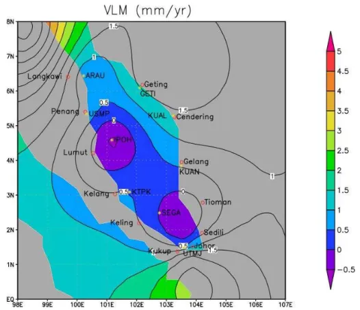
Noticeable rates of VLM have been detected in the Peninsular Malaysia (Simons

et al., 2007), spanning from a subsidence rate of −0.60±2.89 mm yr−1 to an uplift

value of 1.70±1.90 mm yr−1. Although being of the same order as regional SLR rates,

VLM was unlikely accounted for by Peng et al. (2013). For instance, the SLR rate in 25

(5)

OSD

11, 1519–1541, 2014

Q. H. Luu et al.

Title Page

Tables Figures

◭ ◮

Back Close

Full Screen / Esc

Discussion

P

a

per

|

Discus

sion

P

a

per

|

Discussion

P

a

per

|

Discussion

P

a

per

|

with VLM correction is clearly required to derive robust sea level trend around the Peninsular Malaysia.

Meanwhile, at interannual scale, the ENSO is a renowned climatic driver governing sea level variability over the tropical Pacific. In the SCS, interannual sea level variability has a strong signature of the ENSO (Wang et al., 2006; Cheng and Qi, 2007; Rong 5

et al., 2007; Chen et al., 2012; Tkalich et al., 2013; Peng et al., 2013). In the Singapore

Strait, sea level anomaly (SLA) is highly correlated (−0.7) with the Multivariate ENSO

Index (MEI) during the observation period (1984–2011). Drops and rises of mean sea

level (MSL) in the strait in the order of ±5 cm are associated with El Niño and La

Niña episodes, respectively (Tkalich et al., 2013). The influence of ENSO becomes 10

stronger toward southern region of the SCS (Rong et al., 2007; Peng et al., 2013). Qu et al. (2004) suggested that the intrusion of Kuroshio Current through the Luzon Strait coupled with atmospheric teleconnection is likely to cause such interannual variability. In the Bay of Bengal and the Andaman Sea, the ENSO alters the MSL within the range of±15 cm (Aparna et al., 2012; Sreenivas et al., 2012).

15

Similar to the ENSO, the Indian Ocean Dipole (IOD) affects sea level as well as

climate of countries surrounding the Indian Ocean basin, extending from eastern Africa to southern Australia (Saji et al., 1999; Iizuka et al., 2000). The west IOD pole exists in the Arabian Sea, while its east pole occurs in the southern sea of Indonesia. The signature of IOD has been detected in the sea level in the Gulf of Bengal, which varies 20

in the range ±20 cm (Aparna et al., 2012; Sreenivas et al., 2012). It is not known to

what extent sea level around the Peninsular Malaysia is affected by the IOD, as it is

shielded behind the Kalimantan and Sumatra Islands.

At seasonal scale, sea level variability across the SCS is predominantly driven by the Asian monsoonal wind (Wyrtki, 1961; Lau et al., 1998; Ding and Johnny, 2005; Tan 25

et al., 2006; Wang et al., 2009; Liang and Evans, 2011). At a closer look, the Asian monsoon is branching to two major parts: the East Asian – Western Pacific (EAWP) Monsoon (Li and Zeng, 2002; Wang et al., 2008) and the South Asian – Indian (SAI)

(6)

OSD

11, 1519–1541, 2014

Q. H. Luu et al.

Title Page

Tables Figures

◭ ◮

Back Close

Full Screen / Esc

Discussion

P

a

per

|

Discus

sion

P

a

per

|

Discussion

P

a

per

|

Discussion

P

a

per

|

region quite independently (Liang and Evans, 2011). Located in the interferential

do-main, sea level around the Peninsular Malaysia thus may experience monsoon in diff

er-ent ways. Along east coast of Peninsular Malaysia, observed positive SLAs are induced by the wind shear during northeast monsoon (boreal winter), while negative anomalies are caused by the southwest monsoon (Tkalich et al., 2012; Chen et al., 2012). For 5

example, monsoonal wind may increase or decrease the sea level in the Singapore Strait up to 20 cm (Tkalich et al., 2013).

Our aim in this paper is to quantify the sea level trend and variability around the Peninsular Malaysia at various temporal scales, from seasonal to decadal, using research-quality tide gauge data combined with local VLM information and satellite 10

altimetry. Section 2 presents the data, and discusses how sea level variability is con-nected to climate indices. In Sect. 3, sea level variability is quantified at various time-scales, from seasonal pattern to interannual variability and long-term tendency. Main findings are then summarized and discussed in the last section.

2 Data and methodology

15

The annual and monthly sea level data for all considered stations in the domain are ob-tained from the Permanent Service for Mean Sea Level (PSMSL, 2013; Holgate et al., 2013). We use data from 12 research-quality tide gauges out of 25 available at PSMSL, which have more than 20 years of records and minimum gaps. The tide gauges are equally distributed in the domain (Fig. 2): six stations in the Malacca Strait includ-20

ing Langkawi, Pinang, Lumut, Kelang, Keling and Kukup; six stations are located in the eastern Peninsular Malaysia region including Geting, Cendering, Gelang, Tioman, Sedili and Johor Bahru. Representative annual MSL along each side of the Peninsular is averaged using annual MSLs of available stations. Four stations in the Singapore

waters (namely Sultan Shoal, Raffles Lighthouse, Tanjong Pagar and Sembawang) are

25

(7)

OSD

11, 1519–1541, 2014

Q. H. Luu et al.

Title Page

Tables Figures

◭ ◮

Back Close

Full Screen / Esc

Discussion

P

a

per

|

Discus

sion

P

a

per

|

Discussion

P

a

per

|

Discussion

P

a

per

|

In order to get the absolute SLR rate, tide gauge records have to be corrected for VLM. This highly localized phenomenon may occur due to glacial isostatic adjustment (GIA), the dislocation of tectonic plates of the Earth, or solidity of underground soil and sediments. In Malaysia, Simons et al. (2007) reported regional VLM rates during the 1994–2004 period using data from 14 nationwide Global Positioning System (GPS) 5

stations. These values were interpolated by the Kriging method to obtain local VLM rates at tide gauge locations (Fig. 2). Linear trends (Table 1) were obtained by the least square fitting to straight lines, and uncertainties (±) were calculated at 95 % confidence

level.

In correlating interannual sea level variability to ENSO and IOD events, the Multi-10

variate ENSO Index (MEI, 2013) and the Dipole Mode Index (DMI, 2013), respectively, are used as proxies. The MEI index comprises of six main physical variables (sea level pressure, zonal and meridional components of the surface wind, sea surface tempera-ture, surface air temperature and total cloudiness fraction of the sky), which have been measured over the North Pacific for many years (Wolter and Timlin, 1993, 1998). The 15

DMI index is represented by the anomalous sea surface temperature gradient between two areas: a western pole in the Arabian Sea and an eastern pole in the eastern Indian Ocean south of Indonesia (Saji et al., 1999).

Gappy data may lead to incorrect estimates of MSL trend (Douglas, 2001; Wahl et al., 2010: Becker et al., 2012). Around the Peninsular Malaysia, gappy data are seen 20

at all 12 considered stations, where (for instance) Lumut tide gauge records miss as much as 25 % data since 1993. Due to a strong seasonal variability of sea level, even one month gap necessitates removal of the respective year out of trend analysis. At the same time, the gappy years cannot be simply neglected because annual increment due to SLR could be one order smaller than annual and interannual sea level variability. 25

(8)

OSD

11, 1519–1541, 2014

Q. H. Luu et al.

Title Page

Tables Figures

◭ ◮

Back Close

Full Screen / Esc

Discussion

P

a

per

|

Discus

sion

P

a

per

|

Discussion

P

a

per

|

Discussion

P

a

per

|

Peninsular Malaysia is highly correlated with ENSO, and at some regions (i.e., Malacca Strait) partly linked to IOD, the technique could be applied to the extended domain. Here, it is assumed that total annual sea level anomaly is the arithmetic sum of sea level constituents associated with ENSO and IOD, where each constituent is repre-sented as a linear function of corresponding proxy index (MEI and DMI, respectively). 5

Least-square minimal algorithm is applied in order to fit linear parameters. The derived function is then used to fill the missing data in the respective years.

To assess the reconstruction algorithm, satellite altimetry observation (AVISO, 2013) during the common period (1993–2011) is used as a baseline. Improvement of recon-structed data over original PSMSL records is small at most individual gauges; how-10

ever, the total accumulative di_fference is clearly seen at averaged trend for each side of the Peninsular. For example, original data for the period 1993–2009 show sea level trend (−0.2) mm yr−1 (Malacca Strait) and 2.5 mm yr−1 (eastern Peninsular Malaysia);

whereas, respective reconstructed values (3.2 mm yr−1

and 3.6 mm yr−1

) are

signifi-cantly closer to altimetry trend 3.6 mm yr−1 during the same period (see also Table 1

15

and Sect. 3.3).

3 Results and discussions

3.1 Seasonal sea level variability

Figure 3 presents the seasonal pattern of sea level at different regions around the

Peninsular Malaysia. Sea level varies at the eastern coast of Peninsular Malaysia in 20

the range of ±25 cm throughout a year, yielding single peak during Northeast (NE)

(9)

OSD

11, 1519–1541, 2014

Q. H. Luu et al.

Title Page

Tables Figures

◭ ◮

Back Close

Full Screen / Esc

Discussion

P

a

per

|

Discus

sion

P

a

per

|

Discussion

P

a

per

|

Discussion

P

a

per

|

and along east coast of Peninsular Malaysia. During summer months, SW wind pulls water mass offthe Sunda Shelf, leading to the drop of sea level.

In the Malacca Strait, quasi-periodic annual cycle is observed twice a year within

the range of±15 cm (Fig. 3a). Positive peaks are observed during May and November,

while negatives are seen during February–March and September. The complexity of 5

the pattern is arguably due to competing of the seasonal wind from the SCS with the wind curl from the Andaman Sea blowing toward the Malacca Strait. Liang and Evans (2011) pointed out that this region is influenced by the SAI monsoon, which regulates local dynamics independently from the EAWP monsoon.

Singapore Strait sea level records (Fig. 3b, after Tkalich et al., 2013) show transient 10

features of both sides of Peninsular Malaysia. The node is located between Ra_ffles

Lighthouse and Tanjong Pagar stations, most likely at the narrowest part of Singapore Strait.

3.2 Interannual sea level variability

Figure 4 presents the interannual variability of sea level around the Peninsular Malaysia 15

during the observation period. Averaged annual sea level at different parts of the

do-main as well as annual records from individual tide gauges are highly correlated with MEI, as in Figs. 5 and 6, respectively. Sea levels in the Malacca Strait have slightly larger correlations with MEI with an average of (−0.69) and the largest of (−0.73) at

Kelang and Pinang tide gauges; while arithmetic mean of correlations in the eastern 20

Peninsular Malaysia is (−0.64). Prominent annual sea level troughs are clearly

ob-served during extreme El Niño episodes in the years 1987, 1991–1992, 1997, 2002, 2006 and 2009; while sea level peaks are tangible amongst La Niña phases in the years 1988–1989, 1996, 1999 and 2008. The magnitude of annual sea level variability is proportional to the intensity of ENSO events. During extreme periods of El Niño or 25

(10)

OSD

11, 1519–1541, 2014

Q. H. Luu et al.

Title Page

Tables Figures

◭ ◮

Back Close

Full Screen / Esc

Discussion

P

a

per

|

Discus

sion

P

a

per

|

Discussion

P

a

per

|

Discussion

P

a

per

|

most likely due to a combination of signals from atmospheric teleconnection feedback and oceanic lateral fluxes.

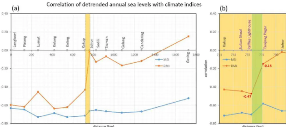
Whilst ENSO signatures are evident at most of tide gauge records along the Malaysian coasts, the IOD signals are detected merely in the Malacca Strait. The

cor-relation between sea level change and DMI is significant (−0.5) along the Malacca

5

Strait (Fig. 6). As a secondary force, extreme IOD events may raise or lower sea level by 2 cm. Explanation for how IOD drives the sea level change is also not well revealed – probably through the easterly zonal wind-induced equatorial Kelvin waves generated in the Indian Ocean during IOD events and propagating to Malacca Strait through the Andaman Sea (Vinaychandran et al., 1999; Mutrugudde et al., 2000).

10

The correlation coe_fficient between DMI and annual sea level in the Malacca Strait

gradually decreases eastward from Andaman Sea toward Singapore Strait, being

(−0.60) at Langkawi tide gauge, (−0.43) at Kukup, and (−0.02) at Johor (Fig. 6a).

Zooming into the Singapore waters, a sharp reduction of correlation is observed be-tween Raffles Lighthouse (−0.47) and Tanjong Pagar (−0.15) as shown in Fig. 6b. It is 15

coincident with the separation found in the seasonal variations of sea level (Sect. 3.1), which may be explained by the fact that IOD evolution is locked to seasonal changes (Toshio et al., 2003).

The concurrence of ENSO and IOD impacts may strengthen the sea level anomaly. For instance, in 1997 when both MEI and DMI gained their highest positive values, sea 20

level in the Malacca Strait dropped more than 7 cm on average (Fig. 5). Sea level drop up to 10 cm is observed at Langkawi, Pinang and Kelang stations (Fig. 4), which are more exposed to the IOD impact due to the geographic location (Fig. 6).

3.3 Long-term sea level trend

During the period 1984–2011, relative SLR rates in the Malacca Strait and eastern 25

Peninsular Malaysia have been 2.4±1.6 mm yr−1 and 2.7±1.0 mm yr−1, respectively

(Table 1); which is lower than to the speed 3.2±1.2 mm yr−1 observed in the

(11)

OSD

11, 1519–1541, 2014

Q. H. Luu et al.

Title Page

Tables Figures

◭ ◮

Back Close

Full Screen / Esc

Discussion

P

a

per

|

Discus

sion

P

a

per

|

Discussion

P

a

per

|

Discussion

P

a

per

|

was estimated from reconstruction dataset as 3.9±0.6 mm yr−1 (Peng et al., 2013);

while Singapore Strait records exhibited an increment of 3.4 ± 2.4 mm yr−1 (Tkalich

et al., 2013). These regional relative rates are significantly higher than measurements in the Malaysia Peninsular for the same years (Malacca Strait: 2.7±3.6 mm yr−1;

east-ern Peninsular Malaysia: 2.2±1.9 mm yr−1). 5

Taking into account the VLM, absolute SLR rates obtained from Peninsular Malaysia

tide gauges for the 1984–2011 era are 3.2±4.2 mm yr−1 (Malacca Strait) and 3.6±

3.2 mm yr−1 (eastern Peninsular Malaysia), as shown in Table 1. For the common

pe-riod 1993–2009, both satellite altimetry and corrected tidal record show similar abso-lute SLR rates. In the Malacca Strait, estimates are 3.4±6.2 mm yr−1(tide gauges) and 10

3.6±2.7 mm yr−1(satellite data); while at the eastern coast of Peninsular Malaysia, they

are 3.1±4.1 mm yr−1and 3.6±1.6 mm yr−1, respectively. These rates are slightly higher

than the global tendencies observed from tide gauges (2.8±0.8 mm yr−1, Church and

White, 2011) and satellite altimetry (3.3±0.4 mm yr−1, Nicholls and Cazenave, 2010)

for the same years. 15

Present in situ estimate of global SLR rates mostly rely on the GIA, which is solely applicable to correct VLM in polar region (Church and White, 2006, 2011). As no correc-tion is applied to tide gauges beyond this region such as around equatorial areas, the global estimate of SLR rate could be improved with local VLM information. As shown in the above example, corrected SLR rate around the Peninsular Malaysia is about 30 % 20

higher than the relative speed measured directly at tide gauges. Meanwhile, present network of GPS stations is sparse and recent (for instance, only 10 year VLM data are available for the Malaysia region). Accordingly, our study underlines the fact that more

efforts should be put forward in the future to measure the VLM in addition to the tide

(12)

OSD

11, 1519–1541, 2014

Q. H. Luu et al.

Title Page

Tables Figures

◭ ◮

Back Close

Full Screen / Esc

Discussion

P

a

per

|

Discus

sion

P

a

per

|

Discussion

P

a

per

|

Discussion

P

a

per

|

4 Conclusions

Tide gauge records, satellite altimetry data, VLM as well as climate proxies are used to quantify sea level trend and variability along Peninsular Malaysia coast. It is found that during 1984–2011 years, relative sea level rise (SLR) rates at Malacca

Strait and eastern coast of Peninsular Malaysia are found to be 2.4±1.6 mm yr−1and

5

2.7±1.0 mm yr−1, respectively. Allowing for corresponding VLMs (0.8±2.6 mm yr−1and

0.9±2.2 mm yr−1), their absolute SLR rates are 3.2±4.2 mm yr−1and 3.6±3.2 mm yr−1,

respectively. For the common period 1993–2009, absolute SLR rates obtained from tide gauges and satellite altimetry along Peninsular Malaysia coast are similar; and they are slightly higher than the global tendency. This result underlines the fact VLM must be 10

taken into account to get better estimates of in situ SLR observations.

At interannual scale, ENSO modulates sea level variability around the peninsular,

while IOD affects the west coast (Malacca Strait) mainly. Interannual regional sea

level drops are associated with El Niño events, while the rises are correlated with La Niña episodes; both variations are in the range of±5 cm having correlation coefficient 15

of (−0.7) with respect to MEI. The IOD modulates interannual sea level variability in

the Malacca Strait in the range of±2 cm with a correlation coefficient (−0.5) relative to

DMI. At annual scale, SLAs are mainly monsoon-driven, in the order of 10–25 cm. They

respond differently to the Asian monsoon; having two quasi-periodic cycles annually in

the Malacca Strait, presumably due to South Asian-Indian Monsoon; but a single one 20

annually in the remaining region, mostly due to East Asian-Western Pacific Monsoon. We suggest that a topographical and hydrodynamic constriction located between Raf-fles Lighthouse and Tanjong Pagar tide gauges in the Singapore Strait may separate sea level variabilities observed at both sides of the Peninsular Malaysia.

Acknowledgements. We thank J. Huthnance and B. Thompson for useful suggestions, and

25

(13)

OSD

11, 1519–1541, 2014

Q. H. Luu et al.

Title Page

Tables Figures

◭ ◮

Back Close

Full Screen / Esc

Discussion

P

a

per

|

Discus

sion

P

a

per

|

Discussion

P

a

per

|

Discussion

P

a

per

|

References

Aparna, S. G., McCreary, J. P., Shankar, D., and Vinayachandran, P. N.: Signatures of Indian Ocean dipole and El Niño–Southern Oscillation events in sea level variations in the Bay of Bengal, J. Geophys. Res., 117, C10012, doi:10.1029/2012JC008055, 2012.

AVISO: Altimetric data, available at: http://www.aviso.oceanobs.com/en/data.html (last access:

5

25 January 2013), 2013.

Becker, M., Meyssignac, B., Letetrel, C., Llovel, W., Cazenave, A., and Delcroix, T.: Sea level variations at tropical Pacific islands since 1950, Global Planet. Change, 80–81, 85–98, doi:10.1016/j.gloplacha.2011.09.004, 2012.

Chen, H., Tkalich, P., Malanotte-Rizzoli, P., and Wei, J.: The forced and free response of

10

the South China Sea to the large-scale monsoon system, Ocean Dynam., 62, 377–393, doi:10.1007/s10236-011-0511-7, 2012.

Cheng, X. and Qi, Y.: Trends of sea level variations in the South China Sea from merged altimetry data, Global Planet. Change, 57, 371–382, doi:10.1016/j.gloplacha.2007.01.005, 2007.

15

Church, J. A. and White, N. J.: A 20th century acceleration in global sea-level rise, Geophys. Res. Lett., 33, L01602, doi:10.1029/2005GL024826, 2006.

Church, J. A. and White, N. J.: Sea-level rise from the late 19th to the early 21st century, Surv. Geophys., 32, 585–602, doi:10.1007/s10712-011-9119-1, 2011.

Ding, Y. and Johnny, C. L. C.: The East Asian summer monsoon: an overview, Meteorol. Atmos.

20

Phys., 89, 117–142, doi:10.1007/s00703-005-0125-z, 2005.

DMI: Dipole Mode Index, available at: http://stateoftheocean.osmc.noaa.gov/sur/ind/dmi.php (last access: 28 July 2013), 2013.

Douglas, B. C.: Sea level change in the era of the recording tide gauge, in: Sea Level Rise: History & Consequence, edited by: Douglas, B. C., Kearney, M. S., and Leatherman, S. P.,

25

International Geophysical Series, 75, Academic Press, 37–64, 2001.

Goswami, B. N., Krishnamurthy, V., and Annmalai, H.: A broad-scale circulation index for the interannual variability of the Indian summer monsoon, Q. J. Roy. Meteorol. Soc., 125, 611– 633, doi:10.1002/qj.49712555412, 1999.

Holgate, S. J., Matthews, A., Woodworth, P. L., Rickards, L. J., Tamisiea, M. E.,

Brad-30

(14)

OSD

11, 1519–1541, 2014

Q. H. Luu et al.

Title Page

Tables Figures

◭ ◮

Back Close

Full Screen / Esc

Discussion

P

a

per

|

Discus

sion

P

a

per

|

Discussion

P

a

per

|

Discussion

P

a

per

|

and products at the permanent service for mean sea level, J. Coastal Res., 29, 493–504, doi:10.2112/jcoastres-d-12-00175.1, 2013.

Iizuka, S., Matsuura, T., and Yamagata, T.: The Indian Ocean SST dipole simulated in a coupled general circulation model, Geophys. Res. Lett., 27, 3369–3372, doi:10.1029/2000GL011484, 2000.

5

Jevrejeva, S., Moore, J. C., Grinsted, A., and Woodworth, P. L.: Recent global sea level acceleration started over 200 years ago?, Geophys. Res. Lett., 35, L08715, doi:10.1029/2008GL033611, 2008.

Laing, A. and Evans, J. L.: Introduction to Tropical Metorology, 2nd Edn., COMET Pro-gram, available at: http://www.goes-r.gov/users/comet/tropical/textbook_2nd_edition/index.

10

htm (last access: 14 March 2014), University Corporation for Atmospheric Research, 2011. Lau, K.-M., Wu, H.-T., and Yang, S.: Hydrologic processes associated with the first transition of

the Asian Summer Monsoon: a pilot satellite study, B. Am. Meteorol. Soc., 79, 1871–1882, doi:10.1175/1520-0477(1998)079<1871:HPAWTF>2.0.CO;2, 1998.

Li, J. and Zeng, Q.: A unified monsoon index, Geophys. Res. Lett., 29, 1274,

15

doi:10.1029/2001GL013874, 2002.

Luu, Q. H. and Tkalich, P.: Reconstruction of gappy mean sea level data, in: Proceedings of the Fifth Indian Nat. Conf. Harbour Ocean Eng., Goa, India, 5–7 February, 5 pp., 2014.

Murtugudde, R., McCreary, J. P., and Busalacchi, A. J.: Oceanic processes associated with anomalous events in the Indian Ocean with relevance to 1997–1998, J. Geophys. Res., 105,

20

3295–3306, 2000.

MEI: Multivariate ENSO Index, available at: http://www.esrl.noaa.gov/psd/enso/mei/ (last ac-cess: 25 July 2013), 2013.

Meyssignac, B., Becker, M., Llovel, W., and Cazenave, A.: An assessment of two-dimensional past sea level reconstructions over 1950–2009 based on tide-gauge data and different input

25

sea level grids, Surv. Geophys., 33, 945–972, doi:10.1007/s10712-011-9171-x, 2012. Nerem, R. S., Leuliette, E., and Cazenave, A.: Present-day sea-level change: a review, Ext.

Geophys. Clim. Env., 338, 1077–1083, doi:10.1016/j.crte.2006.09.001, 2006.

Nerem, R. S., Chambers, D., Choe, C., and Mitchum, G. T.: Estimating mean sea level change from the TOPEX and Jason altimeter missions, Mar. Geod., 33, 435–446,

30

doi:10.1080/01490419.2010.491031, 2010.

(15)

OSD

11, 1519–1541, 2014

Q. H. Luu et al.

Title Page

Tables Figures

◭ ◮

Back Close

Full Screen / Esc

Discussion

P

a

per

|

Discus

sion

P

a

per

|

Discussion

P

a

per

|

Discussion

P

a

per

|

Peng, D., Palanisamy, H., Cazenave, A., and Meyssignac, B.: Interannual sea level variations in the South China Sea over 1950–2009, Mar. Geod., 36, 164–182, doi:10.1080/01490419.2013.771595, 2013.

PSMSL: Obtaining Tide Gauge Data, available at: http://www.psmsl.org/data/obtaining/ (last access: 28 June 2013), 2013.

5

Rao, S. A., Behera, S. K., Masumoto, Y., and Yamagata, T.: Interannual subsurface variability in the tropical Indian Ocean with a special emphasis on the Indian Ocean dipole, Deep-Sea Res. Pt. II, 49, 1549–1572, doi:10.1016/S0967-0645(01)00158-8, 2002.

Rong, Z., Liu, Y., Zong, H., and Cheng, Y.: Interannual sea level variability in the South China Sea and its response to ENSO, Global Planet. Change, 55, 257–272,

10

doi:10.1016/j.gloplacha.2006.08.001, 2007.

Saji, N. H., Goswami, B. N., Vinayachandran, P. N., and Yamagata, T.: A dipole mode in the tropical Indian Ocean, Nature, 401, 360–363, 1999.

Simons, W. J. F., Socquet, A., Vigny, C., Ambrosius, B. A. C., Haji Abu, S., Promthong, C., Subarya, C., Sarsito, D. A., Matheussen, S., Morgan, P., and Spakman, W.: A decade of

15

GPS in Southeast Asia: resolving Sundaland motion and boundaries, J. Geophys. Res., 112, B06420, doi:10.1029/2005JB003868, 2007.

Sreenivas, P., Gnanaseelan, C., and Prasad, K. V. S. R.: Influence of El Niño and Indian Ocean Dipole on sea level variability in the Bay of Bengal, Global Planet. Change, 80–81, 215–225, doi:10.1016/j.gloplacha.2011.11.001, 2012.

20

Stammer, D., Cazenave, A., Ponte, R. M., and Tamisiea, M. E.: Causes for contemporary regional sea level changes, Annu. Rev. Mar. Sci., 5, 21–46, doi:10.1146/annurev-marine-121211-172406, 2013.

Tan, C. K., Ishizaka, J., Matsumura, S., Yusoff, F. M., Mohamed, M. I. H.: Seasonal variability of SeaWiFS chlorophyll a in the Malacca Straits in relation to Asian monsoon, Cont. Shelf

25

Res., 26, 168–178, doi:10.1016/j.csr.2005.09.008, 2006.

Tkalich, P., Vethamony, P., Babu, M. T., and Malanotte-Rizzoli, P.: Storm surges in the Singapore Strait due to winds in the South China Sea, Nat. Hazards, 66, 1345–1362, doi:10.1007/s11069-012-0211-8, 2012.

Tkalich, P., Vethamony, P., Luu, Q.-H., and Babu, M. T.: Sea level trend and variability in the

30

(16)

OSD

11, 1519–1541, 2014

Q. H. Luu et al.

Title Page

Tables Figures

◭ ◮

Back Close

Full Screen / Esc

Discussion

P

a

per

|

Discus

sion

P

a

per

|

Discussion

P

a

per

|

Discussion

P

a

per

|

Toshio, Y., Behera, S. K., Rao, S. A., Guan, Z., Ashok, K., and Saji, H. N.: Comments on “Dipoles, Temperature Gradients, and Tropical Climate Anomalies”, B. Am. Meteorol. Soc., 84, 1418–1422, doi:10.1175/BAMS-84-10-1418, 2003.

Trisirisatayawong, I., Naeije, M., Simons, W., and Fenoglio-Marc, L.: Sea level change in the Gulf of Thailand from GPS-corrected tide gauge data and multi-satellite altimetry, Global

5

Planet. Change, 76, 137–151, doi:10.1016/j.gloplacha.2010.12.010, 2011.

Vinayachandran, P. N., Saji, N. H., and Toshio, Y.: Response of the equatorial Indian Ocean to an unusual wind event during 1994, Geophys. Res. Lett., 26, 1613–1616, doi:10.1029/1999GL900179, 1999.

Wahl, T., Jensen, J., and Frank, T.: On analysing sea level rise in the German Bight since 1844,

10

Nat. Hazards Earth Syst. Sci., 10, 171–179, doi:10.5194/nhess-10-171-2010, 2010.

Wang, B. and Fan, Z.: Choice of South Asian summer monsoon indices, B. Am. Meteorol. Soc., 80, 629–638, 1999.

Wang, B., Huang, F., Wu, Z., Yang, J., Fu, X., and Kikuchi, K.: Multi-scale climate vari-ability of the South China Sea monsoon: a review, Dynam. Atmos. Oceans, 47, 15–37,

15

doi:10.1016/j.dynatmoce.2008.09.004, 2009.

Wang, C., Wang, W., Wang, D., and Wang, Q.: Interannual variability of the South China Sea associated with El Niño, J. Geophys. Res.-Oceans, 111, 2156–2202, doi:10.1029/2005JC003333, 2006.

Wolter, K. and Timlin, M. S.: Monitoring ENSO in COADS with a seasonally adjusted

prin-20

cipal component index, in: Proceedings of the 17th Clim. Diagn. Workshop, Norman, OK, NOAA/NMC/CAC, NSSL, Oklahoma Climate Survey, CIMMS and School of Meteorology, University Oklahoma, 52–57, 1993.

Wolter, K. and Timlin, M. S.: Measuring the strength of ENSO events – how does 1997/98 rank?, Weather, 53, 315–324, doi:10.1002/j.1477-8696.1998.tb06408.x, 1998.

25

(17)

OSD

11, 1519–1541, 2014

Q. H. Luu et al.

Title Page Abstract Introduction Conclusions References Tables Figures ◭ ◮ ◭ ◮ Back Close

Full Screen / Esc

Printer-friendly Version Interactive Discussion Discussion P a per | Discus sion P a per | Discussion P a per | Discussion P a per |

Table 1.Linear trends (mm yr−1

) of SLR and VLM rates over selected periods.

SLR rate from tide gauge record

Source of record Entire period 1993–2009 SLR rate from satellitei _{VLM rate}a,h

(Location) Period Relative Absolutei Relative Absolutei 1993–2011 1993–2009 1994–2004

Langkawi (99◦

46′ E, 6◦

26′

N) 1986–2011 3.0±2.0 4.4±4.7 1.9±4.2 3.3±6.9 3.4±2.6 2.8±3.2 1.4±2.7

Pinang (100◦

21′ E, 5◦

27′

N) 1986–2011 3.7±2.1 4.5±5.8 4.4±4.4 5.2±8.1 3.3±2.3 2.7±2.8 0.8±3.7

Lumut (100◦

37′ E, 4◦

14′

N) 1985–2010 2.1±1.7 2.0±4.4 2.2±3.5 2.1±6.2 4.3±2.6 3.8±3.2 −0.1±2.7

Kelang (101◦₂₁′_{E, 3}◦₀₃′_N) _1984–2011 _1.8

±1.8 2.3±4.1 1.4±3.8 2.0±6.1 4.1±2.7 3.3±3.2 0.5±2.3

Keling (102◦₀₉′_{E, 2}◦₁₃′_N) _1985–2011 _2.4

±1.7 2.9±4.0 2.9±3.6 3.4±5.9 4.7±2.1 4.5±2.7 0.5±2.3

Kukup (103◦₂₇′_{E, 1}◦₂₀′_N) _1986–2011 _3.0

±1.6 4.4±3.6 3.3±3.3 4.7±5.3 5.2±2.2 4.5±2.7 1.4±2.0

Malacca Strait 1984–2011 2.4±1.6 3.2±4.2 2.7±3.6 3.4±6.2 4.1±2.2 3.6±2.7 0.8±2.6

Johor (103◦₄₈′_{E, 1}◦₂₈′_N) _1984–2011 _2.3

±1.1 3.5±3.1 1.9±2.3 3.1±4.3 5.0±2.1 4.2±2.6 1.2±2.0

Sedili (104◦₀₇′_{E, 1}◦₅₆′_N) _1987–2011 _2.5

±1.2 2.8±3.3 1.8±2.1 2.1±4.2 4.0±1.5 3.5±1.7 0.3±2.1

Tioman (104◦₀₈′_{E, 2}◦₄₈′_N) _1986–2011 _3.0

±1.2 3.3±3.5 2.6±2.0 2.9±4.3 4.0±1.4 3.4±1.6 0.3±2.3

Gelang (103◦₂₆′_{E, 3}◦₅₉′_N) _1984–2011 _3.2

±1.0 3.8±3.4 3.5±1.8 4.1±4.2 3.9±1.5 3.4±1.8 0.6±2.4

Cendering (103◦₁₁′_{E, 5}◦₁₆′_N) _1985–2011 _3.3

±1.1 4.7±2.6 2.3±2.0 3.7±3.5 3.9±1.4 3.2±1.6 1.4±1.5

Geting (102◦₀₆′_{E, 6}◦₁₄′_N) _1987–2011 _3.1

±1.5 4.7±4.2 1.1±2.4 2.7±5.1 4.4±1.4 3.9±1.7 1.6±2.7

Eastern Peninsular Malaysia 1984–2011 2.7±1.0 3.6±3.2 2.2±1.9 3.1±4.1 4.2±1.4 3.6±1.6 0.9±2.2

Singapore Straitb 1984–2011 3.2±1.2 3.4±2.4

Gulf of Thailandc 1940–2004 3.0±1.5 3.6±0.7

South China Sead _1950–2009 _1.7

±0.1 3.9±0.6

Global tidal gaugee 1900–2009 1.7±0.2 2.8±0.8

Global altimetry 1993–2013 3.2±0.4f _3.3

±0.4g

a

VLM rates and uncertainties are interpolated from Simons et al. (2007);

b

Tkalich et al. (2013);

c_{Trisirisatayawong et al. (2011) at Ko Lak tide gauge;} d

Peng et al. (2013);

e

Church and White (2011);

f

Nerem et al. (2010);

g

Nicholls and Cazenave (2010);

h

Assume that VLM speed is constant beyond its observational period.

i

(18)

OSD

11, 1519–1541, 2014

Q. H. Luu et al.

Title Page

Tables Figures

◭ ◮

Back Close

Full Screen / Esc

Discussion

P

a

per

|

Discus

sion

P

a

per

|

Discussion

P

a

per

|

Discussion

P

a

per

|

(19)

OSD

11, 1519–1541, 2014

Q. H. Luu et al.

Title Page

Tables Figures

◭ ◮

Back Close

Full Screen / Esc

Discussion

P

a

per

|

Discus

sion

P

a

per

|

Discussion

P

a

per

|

Discussion

P

a

per

|

Figure 2.Locations of and GPS stations (yellow symbols) extracted from Simons et al. (2007) and tidal gauge stations (red circles) archived from PSMSL (2013) along the coasts of Penin-sular Malaysia. Contours represent VLM rates (mm yr−1

(20)

OSD

11, 1519–1541, 2014

Q. H. Luu et al.

Title Page

Tables Figures

◭ ◮

Back Close

Full Screen / Esc

Discussion

P

a

per

|

Discus

sion

P

a

per

|

Discussion

P

a

per

|

Discussion

P

a

per

|

(21)

OSD

11, 1519–1541, 2014

Q. H. Luu et al.

Title Page

Tables Figures

◭ ◮

Back Close

Full Screen / Esc

Discussion

P

a

per

|

Discus

sion

P

a

per

|

Discussion

P

a

per

|

Discussion

P

a

per

|

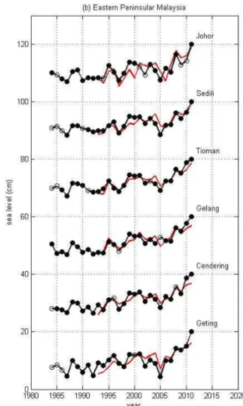
Figure 4.Annual sea level at tidal gauges around the Peninsular Malaysian:(a)Malacca Strait,

(22)

OSD

11, 1519–1541, 2014

Q. H. Luu et al.

Title Page

Tables Figures

◭ ◮

Back Close

Full Screen / Esc

Discussion

P

a

per

|

Discus

sion

P

a

per

|

Discussion

P

a

per

|

Discussion

P

a

per

|

(23)

OSD

11, 1519–1541, 2014

Q. H. Luu et al.

Title Page

Tables Figures

◭ ◮

Back Close

Full Screen / Esc

Discussion

P

a

per

|

Discus

sion

P

a

per

|

Discussion

P

a

per

|

Discussion

P

a

per

|