Seasonal variability of the Caspian Sea three-dimensional circulation, sea level and air-sea interaction

(1)

OSD

6, 1913–1970, 2009

Seasonal variability of the Caspian Sea

three-dimensional circulation

R. A. Ibrayev et al.

Title Page

Abstract Introduction

Conclusions References

Tables Figures

◭ ◮

Back Close

Full Screen / Esc

Printer-friendly Version

Interactive Discussion Ocean Sci. Discuss., 6, 1913–1970, 2009

www.ocean-sci-discuss.net/6/1913/2009/

Ocean Science Discussions

Papers published inOcean Science Discussionsare under open-access review for the journalOcean Science

Seasonal variability of the Caspian Sea

three-dimensional circulation, sea level

and air-sea interaction

R. A. Ibrayev1,2, E. ¨Ozsoy3, C. Schrum4, and H. ˙I. Sur5

1

Institute of Numerical Mathematics, Russian Academy of Sciences, Moscow, Russia

2

P. P. Shirshov Institute of Oceanology, Russian Academy of Sciences, Moscow, Russia

3

Institute of Marine Sciences, Middle East Technical University, Erdemli-Mersin, Turkey

4

Geophysical Institute, The University of Bergen, Bergen, Norway

5

Institute of Marine Sciences and Operation, Istanbul University, Istanbul, Turkey

Received: 10 June 2009 – Accepted: 30 June 2009 – Published: 1 September 2009 Correspondence to: R. A. Ibrayev (ibrayev@inm.ras.ru)

(2)

OSD

6, 1913–1970, 2009

Title Page

Tables Figures

◭ ◮

Back Close

Full Screen / Esc

Interactive Discussion Abstract

A three-dimensional primitive equation model including sea ice thermodynamics and air-sea interaction is used to study seasonal circulation and water mass variability in the Caspian Sea under the influence of realistic mass, momentum and heat fluxes. River discharges, precipitation, radiation and wind stress are seasonally specified in

5

the model, based on available data sets. The evaporation rate, sensible and latent heat fluxes at the sea surface are computed interactively through an atmospheric boundary layer sub-model, using the ECMWF-ERA15 re-analysis atmospheric data and model generated sea surface temperature. The model successfully simulates sea-level changes and baroclinic circulation/mixing features with forcing specified for a

se-10

lected year. The results suggest that the seasonal cycle of wind stress is crucial in producing basin circulation. Seasonal cycle of sea surface currents presents three types: cyclonic gyres in December–January; Eckman south-, south-westward drift in February–July embedded by western and eastern southward coastal currents and tran-sition type in August–November. Western and eastern northward sub-surface coastal

15

currents being a result of coastal local dynamics at the same time play an important role in meridional redistribution of water masses. An important part of the work is the simulation of sea surface topography, yielding verifiable results in terms of sea level. Model successfully reproduces sea level variability for four coastal points, where the observed data are available. Analyses of heat and water budgets confirm climatologic

20

(3)

OSD

6, 1913–1970, 2009

Title Page

Tables Figures

◭ ◮

Back Close

Full Screen / Esc

Interactive Discussion 1 Introduction

The Caspian Sea is the largest totally enclosed water body on Earth, constituting 44% of the global volume of lacustrine waters. Compared to other semi-enclosed and en-closed seas of the world, little is known of the Caspian Sea variability. The most urgent, yet unresolved questions relating to the Caspian Sea are: What is the

three-5

dimensional general circulation of the sea and how does it affect transport of pollutants? How is this circulation created? Through which climatic and dynamic mechanisms is the sea level variability controlled? The phenomenological evidence is too ambiguous or insufficient to give satisfactory answers to these questions.

The Caspian Sea has an elongated geometry (1000 km in length and 200–300 km

10

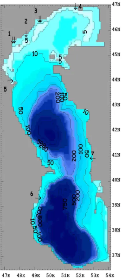
in width), where the Northern, Middle and Southern Caspian Basins (respectively the NCB, MCB and SCB) constitute the main geographic divisions, as illustrated by the model bottom topography in Fig. 3. The shallow NCB has maximum depth of about 20 m, while the MCB and SCB have deep troughs with maximum depths of 788 m and 1025 m respectively. Shelf areas with depth less than 100 m, mainly along the northern

15

and eastern coasts, account for 62% of the total area. The underwater extension of the Apsheron peninsula forms a sill separating the MCB and the SCB, with maximum depth of about 180 m. The SCB contains two thirds and the NCB makes up 1% of the total volume of water (Kosarev and Yablonskaya, 1994).

The sea surface temperature (SST) in the NCB ranges from below zero under frozen

20

ice in winter to 25–26◦C in summer, while more moderate variability occurs in the SCB, changing from 7–10◦C in winter to 25–29◦C in summer. The seasonal thermocline occurs at a depth of 20–30 m during the warm season. Seasonal changes in thermal stratification typically reach a depth of 100 m in the SCB and to 200 m in the MCB, while convection is known to reach the bottom in parts of the MCB during severe winters

25

(Kosarev, 1975).

(4)

OSD

6, 1913–1970, 2009

Title Page

Tables Figures

◭ ◮

Back Close

Full Screen / Esc

Interactive Discussion changes (Terziev et al., 1992). Sharp gradients of salinity occur near the mouths of

rivers such as the Volga, where it changes from 2 to 10, typically at a distance of about 20–100 km from the coast.

The elongated geometry and strong topography of the basin, acted upon by vari-able wind forcing and baroclinic effects result in spatially and temporally variable

cur-5

rents in the Caspian Sea. Despite strong variability of the sea currents, the general circulation has been described to be cyclonic, based on the results of investigations carried out from the end of 19th century till 1950’s, either using indirect estimates of currents (floats, bottles or the dynamic method), or simple hydrodynamic interpreta-tions (Bondarenko, 1993; Terziev et al., 1992). Especially standing out among these

10

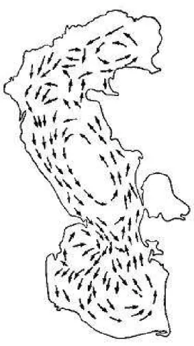
were the six instrumental surveys along the western coast of the MCB, carried out in the years 1935–1937 (Stockman, 1938; Baidin and Kosarev, 1986), showing predomi-nantly southward currents along the western coast of the MCB, modified by wind-driven currents close to the surface. A synthesis of these results has led to the current scheme of Lednev (1943) (Fig. 1).

15

Since the 1950’s, regular oceanographic observations and current measurements in coastal areas shallower than 100 m have confirmed some circulation features illustrated in Fig. 1. Accordingly, the southward currents have been well established along the western coast of MCB; while the northward currents indicated along the eastern coast contradict with summertime observations of surface southward currents in the same

20

region. The cyclonic general circulation of Fig. 1 is partially supported by observed northward currents below of a surface layer (7–8 m depth) of southward drift currents along the eastern coast. It appears that the southward surface currents along the eastern coast are driven by winds with a prevailing southward component in the eastern halves of the MCB and SCB from spring till autumn. The circulation indicated in the

25

shallow NCB appears to be almost totally controlled by local winds (Bondarenko, 1993; Terziev et al., 1992; Kosarev and Yablonskaya, 1994).

(5)

OSD

6, 1913–1970, 2009

Title Page

Tables Figures

◭ ◮

Back Close

Full Screen / Esc

Interactive Discussion of the MCB in summer, expressed by a well-defined pattern of cold water detected in

satellite images (Sur, Ozsoy, and Ibrayev, 1998) and also revealed by climatological temperature fields in the warm season (Kosarev and Tuzhilkin, 1995). Although winter upwelling is also possible under favourable winds, detection by satellite remote sensing becomes more difficult in the cold season, as a result of smaller temperature contrasts

5

with the surrounding waters.

The water budget of the landlocked Caspian Sea is extremely sensitive to climatic variability in the surrounding areas. With a large catchment area extending towards the Urals and Caucasia, river runoffdominates the water budget (with an annual average of∼3×1011m3yr−1 and a range of 2.0–4.5×1011m3yr−1 during the recorded period,

10

Terziev et al. (1992). Annual precipitation is about one third of runoff, while evaporation is of the same order as runoff. Runoff and evaporation each correspond to about 1 m/yr of sea level change. The water budget depends on climate, but anthropogenic effects such as water regulation schemes also had significant effects, leading to inter-annual, inter-decadal and longer term variations in sea level throughout the history of

15

the Caspian Sea (Kosarev and Yablonskaya, 1994; Rodionov, 1994). During 1930– 1977, the sea level decreased to −29 m relative to the mean sea level of the global ocean, from the earlier value of about−26 m lasting from the beginning of the century till the 1930’s. From 1977 onwards, it increased once again to reach the pre-1930’s levels. Rapid sea level change occurred in both of these periods, as indicated in Fig. 2

20

for 1977–1995. Superposed on these inter-decadal changes, the sea level displays a clear seasonal cycle in Fig. 2, as a function of the net water budget (river inflow+

rainfall - evaporation). The sea level reaches its lowest seasonal value in winter and increases in the May–July period, following the spring floods. The climatological mean seasonal range of sea level is about 30 cm (Baidin et al., 1986).

25

(6)

OSD

6, 1913–1970, 2009

Title Page

Tables Figures

◭ ◮

Back Close

Full Screen / Esc

Interactive Discussion surface and river mouths determine the mean sea level in an enclosed water body

such as the Caspian Sea. Surface fluxes of momentum, water and heat are coupled together, and can strongly be modified by the surface temperature and circulation of the sea. On the other hand, these fluxes are the basic elements of the regional hydrological cycle coupled to the global climate. New findings suggest linkages of the Caspian Sea

5

level to ENSO/El Ni ˜no via the Indian Monsoon (Bengtsson, 1998), further supported by predictions of multi-decadal fluctuations and increased river discharges associated with global warming scenarios (Arpe and Roeckner, 1999).

In the past, modelling of the Caspian Sea circulation has been rather limited in scope, relying mostly on diagnostic models. A baroclinic diagnostic model (Sarkisyan,

10

Zaripov, Kosarev, and Rzheplinski, 1976) has shown the importance of wind stress and summer-time thermal stratification in establishing the circulation. The space-time vari-ability of the summer circulation in response to prevailing north-west and south-east winds was studied by Badalov and Rzheplinski (1989), who combined results from non-stationary models of the NCB and of the upper ocean with a diagnostic model of

15

the deep waters. Akhverdiev and Demin (1989), Kosarev and Yablonskaya (1994), and Terziev et al. (1992) presented a number of diagnostic studies of climatic and synop-tic situations. The dynamically adjusted climasynop-tic seasonal circulation investigated by Trukhchev, Kosarev, Ivanova, and Tuzhilkin (1995) and Tuzhilkin, Kosarev, Trukhchev, and Ivanova (1997) showed persistent cyclonic and anticyclonic vortices respectively

20

in the north-west and the south-east sectors of the MCB, and anticyclonic vortices in the north-west and the south-east of the SCB, to be the main elements of the circula-tion. The success of these diagnostic studies was limited by the spatial resolution and quality of the available hydrological data.

Considering the general lack of understanding of the Caspian Sea circulation and

25

(7)

OSD

6, 1913–1970, 2009

Title Page

Tables Figures

◭ ◮

Back Close

Full Screen / Esc

Interactive Discussion A description of the model and its forcing is given in Sects. 2 and 3. In Sect. 4 we

analyse the seasonal circulation, water budget and the resulting sea level variability in correspondence with heat and evaporation fluxes at the air-sea interface. In Sect. 5 we consider the sensitivity of the model results to external forcing and model parameters.

2 Model description

5

2.1 General remarks

The enclosed geometry and size of the Caspian Sea are advantageous for numerical modelling. On the other hand, greater constraints are imposed in formulation of bound-ary fluxes in enclosed basin as compared to semi-enclosed or open seas, as improper accounting of mass or buoyancy fluxes could lead to unrealistic trends of total stored

10

mass, heat and salt in the model.

Sea level change is a direct result of water balance, which depends on the quality of estimation of the river inflows and air-sea water fluxes. River inflows and precipitation, as remotely defined functions, are prescribed in the model, while evaporation depends on local air-sea interaction, i.e. atmospheric parameters (air temperature, humidity,

15

wind speed) near the sea surface and SST. The air-sea interaction module used for computing fluxes is therefore an essential part of the model because systematic errors in mass flux specified otherwise could rapidly contaminate the SST and lead to greatly differing estimates of sea level.

An essential for the model formulation is capability to simulate variability of total

20

water mass in the basin. We use kinematic equation at the sea surface, which make it possible to introduce time-varying thickness of the upper layer in correspondence with the continuity equation.

An important issue concerning the formulation of boundary conditions arise from the fact that fresh water income and outflow plays an important role in the sea dynamics.

25

(8)

OSD

6, 1913–1970, 2009

Title Page

Tables Figures

◭ ◮

Back Close

Full Screen / Esc

Interactive Discussion of 200 years and for the shallow NCB of the order of 1 year. As was discussed by

Beron-Vera, Ochao and Ripa (1999), use of ad hoc surface boundary conditions for salt balance, such as salt relaxation or “virtual” salt flux conditions are unphysical in nature because they create or destroy salt mass. The correct boundary conditions should include the fact that the vast majority of the salt particles remain in the sea

5

during evaporation, and that the precipitated water is essentially pure freshwater. In formulation of boundary conditions for salt, heat and momentum fluxes we follow the approach of Beron-Vera et al. (1999), and of Roulett and Madec (2000) and add to the usual formulation of air-sea fluxes the terms responsible for freshwater influence.

In the study we use free-surface, primitive equation, z-level numerical Model for

En-10

closed Sea Hydrodynamics (MESH), described by Ibrayev (2001), employing Boussi-nesq and hydrostatic approximations. Formulation of free-surface condition in the model allows propagation of surface gravity waves and mean sea surface elevation changes in response to non-zero water balance.

2.2 Governing equations

15

The basic equations of the model in spherical coordinates (λ– longitude,ϕ– latitude, z– depth) are the following:

u_t+(v · ∇)u+wuz−f v+a−1tgϕu2=−(ρ0acosϕ)−1pλ+(Kmuz)z+Du (1) vt+(v · ∇)v+wvz+f u+a−1tgϕuv =−(ρ0a)−1pϕ+(Kmvz)z+Dv (2)

p_z =ρg (3)

20

∇v +wz =0 (4)

Tt+(v · ∇)T +wTz =(KhTz)z+DT +(ρocp)−1Iz·(1−A) (5) S_t+(v· ∇)S+wSz =(KhSz)z+DS (6)

(9)

OSD

6, 1913–1970, 2009

Title Page

Tables Figures

◭ ◮

Back Close

Full Screen / Esc

Interactive Discussion where v=(u, v) is the horizontal velocity vector; w the vertical velocity; T, S, ρ the

temperature, salinity and density of sea water; ρo – mean density; f=2Ωsinϕ the Coriolis parameter, Ω representing the angular velocity of Earth’s rotation; ∇η=(acosϕ)−1[(uη)_λ+(vηcosϕ)_ϕ] the two dimensional gradient operator; K_m, K_h the vertical turbulent viscosity and diffusion coefficients for momentum and scalars;

5

D_u, D_v, D_T, D_S the horizontal turbulent viscosity and diffusion terms for momentum, heat and salinity;athe Earth’s radius;c_pthe specific heat of sea water;Ithe incoming solar irradiance; A – sea ice compactness. The UNESCO equation of state for sea water (UNESCO, 1976) is used in Eq. (7).

For stable stratification, we use Richardson number dependent parameterization of

10

the vertical mixing coefficients proposed by Munk and Anderson (1948):

Km =am0(1+αRi)−n+amb (8)

K_h =a_h0(1+αRi)−n+a_hb (9)

wherea_m0,a_mb,a_h0,a_hb,α,nare empirical constants, andRi is the Richardson num-ber defined asRi=gρzρ−

1 0 [(uz)

2

+(vz) 2

]−1. In the case of unstable stratification, water

15

is mixed instantaneously with conservation of total heat and salt in mixed volumes of water.

Horizontal mixing terms (Du, Dv, DT, DS) expressed in the form Dη=(acosϕ)−1[(Aηηλa−1cos−1ϕ)λ+(Aηηϕa−1cosϕ)ϕ], where η stands for either one of the velocity componentsu, v, temperature or salinity T, S, and A_η stands for

20

the horizontal viscosity (Am) or diffusion (Ah) coefficients, depending on which term is represented.

2.3 Boundary conditions

Sea surface evolution equation taking into account water fluxes is (Kamenkovich, 1973; Ibrayev, 2001):

25

(10)

OSD

6, 1913–1970, 2009

Title Page

Tables Figures

◭ ◮

Back Close

Full Screen / Esc

Interactive Discussion withW=P+M−E, where ζ(λ, ϕ, t) is the sea surface elevation; ρ_f – density of fresh

water;W – water flux;P – precipitation;M – water flux due to ice melting/freezing;E – the rate of evaporation.

Upper boundary conditions are specified at the sea surfacez=ζ(λ, ϕ, t):

−Km(uz, vz)+(u, v)·ρ_f−1W =ρ−o1(1−A)(τλ, τϕ) (11)

5

p=pa (12)

−c_pK_hT_z+c_pT ρ−_f1W =ρ_o−1[Qaw_h (1−A)+Qiw_hA] (13)

−K_hS_z+Sρ−_f1W =ρ−_o1SiwMA (14)

where (τλ, τϕ) are the wind stress components; p_a – atmospheric pressure;Qaw_h , Qiw_h – air-water and ice-water heat fluxes; SiwM the rate of salt flux in the sea due to ice

10

melting/freezing. The second terms of the left side of Eq. (11), Eq. (13), Eq. (14) describe change of salt, heat and momentum content of the surface waters due to fresh water fluxes.

At the sea bottom,z=H(λ, ϕ), the corresponding boundary conditions are: w=u(acosϕ)−1H_λ+va−1_H

ϕ (15)

15

ρoKm(uz, vz)=(τ_Bλ, τ ϕ

B) (16)

Kh(Tz, Sz)=0, (17)

where (τ_Bλ, τ_Bϕ) are the bottom stress components.

At lateral walls, the free slip boundary condition and zero heat and salt fluxes are imposed:

20

vn=0, ∂vτ

(11)

OSD

6, 1913–1970, 2009

Title Page

Tables Figures

◭ ◮

Back Close

Full Screen / Esc

Interactive Discussion A_h(∂T

∂n,

∂S

∂n)=0 (19)

wherenand τ represent respectively the normal and tangential directions to the sur-face. The model has also inflow and outflow open boundaries. At inflow boundaries horizontal velocity components as well as temperature and salinity are prescribed: (u, v, T, S)=(uin_{, v}in_{, T}in_{, S}in₎ ₍₂₀₎

5

while at outflow boundaries only the horizontal velocity components are prescribed

(u, v)=(uout, vout) (21)

and the scalars are allowed to advect out of the region with this velocity. 2.4 Air-sea interaction and sea ice models

The heat fluxes at the sea and ice upper boundaries are the sum of solar surface and

10

long-wave backward radiations, sensible and latent heat fluxes at the sea surface. The momentum, sensible heat and evaporation fluxes are calculated through the air-sea interaction sub-model based on the Monin-Obukhov similarity theory. The bulk transfer coefficients depend on universal functions relevant to the given stability conditions of the atmospheric boundary layer. Inputs for the air-sea interaction sub-model are the

15

air and dew point temperature at 2 m above the sea surface, wind speed at 10 m and the sea surface temperature. The method of iterative flux calculations is based on the approach of Launiainen and Vihma (1990).

Whenever thermal conditions are favourable to form ice, air-sea fluxes are modified to account for the effects of sea-ice, based on the thermodynamic sea-ice sub-model

20

(12)

OSD

6, 1913–1970, 2009

Title Page

Tables Figures

◭ ◮

Back Close

Full Screen / Esc

Interactive Discussion 2.5 Penetration of solar radiation

Although more than half of the incoming solar radiation that enters the ocean in the long wave spectral band is absorbed within the top half meter, the remaining short wave fraction, as it penetrates through the surface waters, modifies SST by absorption, which in turn affects the rate of evaporation, leading to an impact on the water balance

5

of the sea. The subsurface profile for solar radiation is computed using the two-band approximation of Paulson and Simpson (1977):

I(z)=Qs[R·exp(−z/ζ1)+(1−R)·exp(−z/ζ2)] (22) whereQ_s is the downward flux of incoming solar radiation;R is an empirical constant; ζ1, ζ2 are respectively the attenuation lengths for long wave and short wave spectral

10

bands of solar radiation. For a one-dimensional model, Martin (1985) has found his model simulations sensitive to the optical properties of the given type of seawater. For enclosed and semi-enclosed seas, Timofeev (1983) adopts a value ofR=0.53 for the empirical constant. Attenuation lengths for long wave radiation are typically small (we useζ1=0.033 m, as proposed by Timofeev (1983)), so that total absorption occurs in

15

the first model layer. The attenuation length for short wave band of solar radiation strongly depends on turbidity and differs between coastal and offshore regions. For the Caspian Sea its value is estimated to be about 10–15 m in the central parts of the MCB and SCB, and about 1–5 m in the NCB (Terziev et al., 1992). We parameterized the short wave attenuation length as depending on local depth,ζ2=15 m, forH>100 m and

20

ζ2=(15 m/100 m)H, forH<100 m, whereH is the depth of the bottom. 2.6 The model resolution

The grid resolution of the model is (1/12)◦in latitude and (1/9)◦in longitude, which gives a grid size of about 9.3 km. There are 22 vertical model levels defined at depths of 1, 3, 7, 11, 15, 19, 25, 35, 50, 75, 100, 125, 150, 200, 250, 300, 400, 500, 600, 700, 800,

25

(13)

OSD

6, 1913–1970, 2009

Title Page

Tables Figures

◭ ◮

Back Close

Full Screen / Esc

Interactive Discussion The maximum depth in the model is 950 m, and a minimum depth of 5 m occurs in

the shelf region of the NCB. The bottom topography and coastline correspond to the conditions during 1940–1955, when the mean sea level was 28 m below the global ocean level. The model bottom topography in Fig. 3 realistically represents the flat NCB shelf, the steep topographic slopes of the SCB and of the western part of the

5

MCB, as well as a number of islands. 2.7 Initial conditions

The model is initialized from a state of rest corresponding to the climatologic state of the sea in November (Fig. 4) in order to overcome the lack of temperature and salinity data in winter in regions under ice cover.

10

The values of vertical and lateral mixing coefficients were selected to have the following values: (am0, amb, ah0, ahb)=(50.,1.,10.,0.02)×10−4m2s−1, α=1, n=1, A_m=150 m2s−1,A_h=0.1 m2s−1. The time step of integration was 30 min.

We run the model for four years with perpetual seasonal forcing, to ensure that the basin averaged kinetic energy, temperature and general circulation reach

quasi-15

stationary periodical states.

3 External forcing

The model forcing is computed from monthly mean atmospheric surface variables based on the ECMWF ERA15 reanalysis data (wind velocity at 10 m height, air and dew point temperatures at 2 m height, incoming solar radiation and thermal back

radi-20

ation).

We simulate the seasonal dynamics by applying perpetual yearly forcing correspond-ing to a selected year. Since drastic sea level changes in the last two decades have resulted from imbalances in the external forcing, we select a year with the lowest net sea level change in the period of interest covered by the ECMWF data. Analyses

(14)

OSD

6, 1913–1970, 2009

Title Page

Tables Figures

◭ ◮

Back Close

Full Screen / Esc

Interactive Discussion of hydro-meteorological data from Makhachkala, Fort-Shevchenko, Krasnovodsk and

Baku indicate 1982 to be a year with smallest change in mean sea level, amounting to about+6.75 cm from January till December, as shown in Fig. 2. For testing the validity of ECMWF ERA15 data we compare them with climatologic data and statistics from hydrometeorological atlases of Samoilenko and Sachkova (1963) and the books of

5

Kosarev and Yablonskaya (1994) and Terziev et al. (1992) (hereinafter briefly referred to as SS, KY, and TKK).

Monthly mean river runoffdata were obtained from routine hydrometeorological ob-servations.

3.1 Atmospheric forcing

10

3.1.1 Air temperature and humidity

The characteristic air temperature patterns in winter and summer are shown in Fig. 5. In winter, the temperature has a meridional gradient, decreasing from about +8◦C in the SCB to−10◦C in the NCB, with a local minimum near the mountainous west. Air temperature in July has a zonal gradient resulting from contrasts between the desert

15

and mountain regions, increasing from about 22◦C in the northwest to 27◦C in the east. Throughout the year, vapour pressure is higher in the SCB compared to the other sub-basins and also in the interior of the sea compared to the coastal regions. Maxi-mum vapour pressure occurs in July, reaching values of 27 mb and 23 mb respectively at the centers of the SCB and the NCB, and decreasing to 11–15 mb along the eastern

20

coast. In February, the vapour pressure decreases from 8 mb at the center of SCB to 1–2 mb in the NCB and in the coastal regions.

Monthly mean air temperature and vapour pressure distributions for 1982 are close to the climatology provided by TKK, except for winter in the NCB, where air temperature from ECMWF is 3–5◦C higher than the values given by the climatology.

(15)

OSD

6, 1913–1970, 2009

Title Page

Tables Figures

◭ ◮

Back Close

Full Screen / Esc

Interactive Discussion 3.1.2 Wind

The wind speed is typically about 4 m/s during the summer and increases up to 5– 6 m/s in winter. Wind speed in winter increases from south to north, exceeding 6.5 m/s in the north (Fig. 6a). In summer the maximum wind speed occurs to the east of the Apsheron peninsula. The annual cycle of the monthly mean wind can be divided into

5

three periods: a) December–January with convergence of winds in the MCB and SCB resulting from the high land-sea temperature contrast in winter, producing local cells of atmospheric circulation with upward motion of the relatively warmer air in the middle of the basin (Fig. 6a). b) February–July when large-scale anti-cyclonic winds prevail over the Sea (Fig. 6b), with south south-southwest-ward winds and divergence in the SCB.

10

The local atmospheric circulation in summer in the SCB appears to be the opposite of the winter situation, as a result of the reversed land-sea temperature differences, when the land temperature in the surrounding deserts and steppes exceed 30–40◦C, while the sea is relatively cooler. c) August–November, when average wind direction gradually changes from south-, southwest-ward to westward.

15

Substantial agreement is observed between monthly mean winds computed from the ECMWF reanalysis data for 1982 and the climatologic winds provided by SS on the basis of measurements made at ships and 72 coastal meteorological stations. The consistency between the climatologic means of SS from the 1950’s and those derived from ECMWF ERA15 data for the 1980’s suggest relatively small climatic change in

20

the character of winds during the 30 years. 3.1.3 Precipitation

Precipitation over the sea is extremely non-uniform. The southwest receives up to 10 times more rainfall compared to the rest of the basin with a maximum in October and November (Fig. 7a). A maximum value 238 mm/month in November 1982 occurs

25

(16)

OSD

6, 1913–1970, 2009

Title Page

Tables Figures

◭ ◮

Back Close

Full Screen / Esc

Interactive Discussion western part of SCB is normally about 30–40 mm/month (Fig. 7b), but almost

com-pletely vanishes in some years. The annual mean precipitation of 340 mm/month in 1982 is close to the maximum value of 366 mm/month in 1993, and much greater than the minimum of 247 mm/month in 1986. Large-scale precipitation based on ECMWF reanalysis data shows good correlation with the 1900–1960 rainfall data of SS and with

5

the climatologic data of TKK. 3.1.4 Radiation fluxes

Radiation flux for the Caspian Sea has a minimum in December and a maximum that typically occurs in June (Fig. 8). The most distinguishing feature of the net radiation flux pattern is the decrease from west to east in summer. The annual mean net

radia-10

tion flux (defined by the sum of solar and thermal radiation fluxes) is 73 Wm−2 for the ECMWF data set, which is lower than the climatologic estimates of SS (79.7 Wm−2) and of TKK, the latter one having 101–136 Wm−2for different parts of the sea. Annual radiation flux in 1982 is the lowest in the analysed period, which has a maximum of 76.8 Wm−2in 1985.

15

The radiative heat flux plays an important role in the heat and water budgets of the Caspian Sea. Because the net radiation flux of ECMWF reanalysis is lower than the climatological estimates, we have increased the solar radiation by 5% to yield a corrected annual mean net radiation flux of 80.6 Wm−2, a value close to estimate of SS. The sensitivity of the model to radiation flux is further discussed in the following

20

sections.

3.1.5 River forcing

The largest inflow of fresh water comes from the Volga River, accounting for about 80% of the climatological mean river discharge of 250 km3yr−1 (Kosarev and Yablonskaya, 1994). The mass, momentum and buoyancy inputs from the Volga River all play

impor-25

(17)

OSD

6, 1913–1970, 2009

Title Page

Tables Figures

◭ ◮

Back Close

Full Screen / Esc

Interactive Discussion are idealized in the model as shown in Fig. 3. All other sources of freshwater with net

annual water flux greater than 10 km3yr−1, namely the Ural, Terek and Kura rivers are represented by their corresponding discharges of fresh water. The Kara-Bogaz-Gol on the arid eastern coast acts as an important sink in the water balance, largely as a shallow evaporation basin connected to the sea. Altogether, lateral fluxes are specified

5

at 7 input/output ports in the model. Monthly mean runoff for 1982 are specified for the Volga, Ural, Terek and Kura rivers. There was no outflow to Kara-Bogaz-Gol Bay in 1982. Water temperature at all rivers was taken to be the same as the Volga River, using averages for the 1960–1990 period at the Verkhnee Lebjazhie station, reported in the Water Cadastral Reference book of the USSR Rivers. Seasonal variability in

10

Volga river runoff is extremely high. From July till April, the Volga River discharge is about 5000–6000 m3s−1. A sharp increase in run-offof up to 15 500 m3s−1occurs in May–June during the spring flood. Different estimates show that up to 3–5% of Volga runoffmeasured at the Verkhnee Lebjazhie station, located upstream of the delta, is lost due to evaporation in the vast delta of the river (Terziev et al., 1992). To account

15

for this loss, we corrected the Volga river runoff, assuming that the river discharge at the coast amounted to 96% of the inland measurements.

4 Model results

We first consider a basic experiment, and in a later section analyse the sensitivity of the model to external forcing and model parameters. Only the monthly averaged fields are

20

(18)

OSD

6, 1913–1970, 2009

Title Page

Tables Figures

◭ ◮

Back Close

Full Screen / Esc

Interactive Discussion 4.1 Seasonal variability of the Caspian Sea dynamics

4.1.1 Three dimensional currents

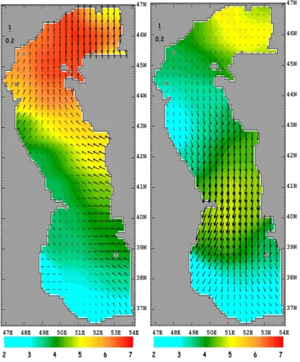
Monthly mean currents at 1 m depth in December, May and August in Fig. 9 exhibit the dominant seasonal patterns of surface circulation. In December and January, sub-basin-scale cyclonic gyres entirely cover the MCB and SCB, while a number of

anti-5

cyclonic and cyclonic eddies are found in the NCB. This pattern of surface currents is expected, in view of the strong westward wind along the eastern coast and the convergence areas in Fig. 6a. The subsurface (25–100 m depth) circulation (Fig. 10) in December and January correlates well with the surface circulation patterns of Fig. 9. Both the MCB and the SCB are occupied by cyclonic gyres connected across the

10

Apsheron sill. Deeper circulation plots reveal that the currents become weaker with depth but preserve their structure all the way to the bottom.

In comparison to the earlier month of December displayed in Fig. 9, the surface circulation first becomes significantly different in February (not shown), when the wind direction changes to become southward in the MCB and SCB. As shown by the May

cir-15

culation in Fig. 9b, the cyclonic gyre in the SCB is shifted to the south and the cyclonic gyre in the MCB disappears. South-southwestward Ekman drift currents dominate the deep-sea regions, superposed on southward coastal currents along the eastern and western shelf regions. The main features of the circulation in May is representative of the period from February till July, which indicates additional small changes in

cur-20

rents along the eastern part of the NCB and cyclonic and anticyclonic eddies near the NCB-MCB boundary.

In February and March the subsurface circulation is gradually modified to become more like Fig. 10b, a pattern which is characteristic of the warm period from April till October. The main differences from the cold period are the appearance of anticyclonic

25

(19)

OSD

6, 1913–1970, 2009

Title Page

Tables Figures

◭ ◮

Back Close

Full Screen / Esc

Interactive Discussion much weaker in the MCB.

Of particular interest is the presence of southward coastal currents along either the eastern and western coasts. Both current systems are dominant from February till July, when the wind-induced southwestward drift currents at the surface result in offshore transport near the east coast and onshore transport near the west coast, resulting in

5

upwelling and downwelling respectively on these coasts to compensate the surface drift. Both current systems span the continental shelf/slope regions in the form of coastal jets studied by Csanady (1982). The coastal current along the west coast and the upwelling along the east are well-documented (Terziev et al., 1992; Kosarev and Yablonskaya, 1994), but often conflicting evidence is found on the eastern coastal

10

current, as a result of its poorly understood horizontal and vertical structure.

The Eastern coastal current near the surface occupies a coastal belt shoreward of the 50 m isobath. At a distance 50–100 km from the coast, the alongshore surface cur-rent turns offshore to join the surface drift, which is compensated by onshore motion in the subsurface layer, as shown in Fig. 11a. In the subsurface layer, slightly offshore

15

of the core of the eastern southward coastal current, exists northward countercurrent, attached to the slope between 50–100 m isobaths, as shown in Fig. 11b. A very sim-ilar, but narrower subsurface current flowing northward takes place under the western coastal current. The core of the counter-current coincides with the pycnocline, which is stronger and shallower in summer.

20

After August, the circulation pattern is gradually modified towards the December pat-tern reviewed earlier. The changes in the circulation are correlated with the changes in wind direction from southward to westward in the MCB and becoming southwestward in the SCB. The earlier southwestward drift in the MCB becomes more west and north-west oriented, as indicated in Fig. 9c. In the north-western part of the MCB, a number of

25

(20)

OSD

6, 1913–1970, 2009

Title Page

Tables Figures

◭ ◮

Back Close

Full Screen / Esc

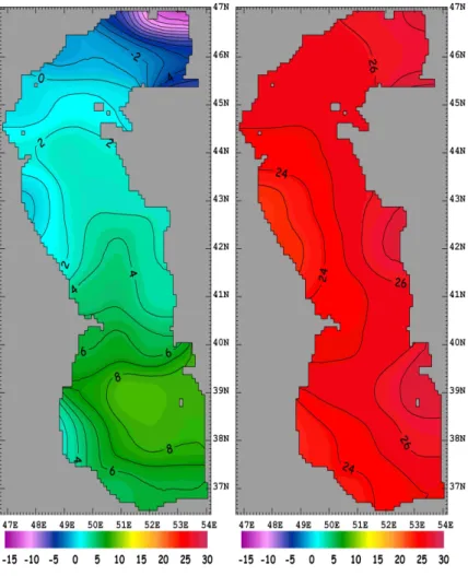
Interactive Discussion 4.1.2 Water mass characteristics

In the shallow NCB, minimum SST occurs in February, when the sea is covered with ice (Fig. 12a). With a time lag, the minimum temperatures in the MCB and SCB occur in March, when the NCB starts warming. The winter time SST increases from lower temperatures near the coast to about 12◦C in the interior of SCB. In autumn and

win-5

ter, the shelf areas are always 5–6◦C cooler than the interior regions, because of the smaller heat capacity of shallow waters.

From December till March, SST in the MCB is characterised by a north-south gra-dient, and tongues of warm water along the eastern coast and cold water along the western coast. In December and January, these coastal SST anomalies are

appar-10

ently related to the cyclonic circulation shown in Figs. 9a and 10a.

A paradox with the tongue of warm water along the eastern coast is that it does not disappear in February and March, at a time when the surface currents (Fig. 9b) are directed southward. The transport of warm water along the coast is maintained by the northward subsurface current identified earlier (Fig. 10b). The warming of surface

15

waters is a result of two mechanisms working in parallel: the upwelling of warm subsur-face vein attached to the shelf (Fig. 11a) and by vertical mixing of this warm subsursubsur-face water with colder surface water.

The west to east increase of SST in the MCB in winter is a characteristic feature of the Caspian Sea climatology (Kosarev and Yablonskaya, 1994). A tongue of warm

20

water extending from the SCB to the MCB along the eastern shelf has been one of the supportive arguments for the existence of the northward current and, hence, of the gen-eral cyclonic circulation pattern at the sea surface. While the surface current system in MCB and SCB in December and January supports the scheme of Fig. 1, then the existence of a southerly flowing coastal current along the east coast and offshore drift

25

(21)

OSD

6, 1913–1970, 2009

Title Page

Tables Figures

◭ ◮

Back Close

Full Screen / Esc

Interactive Discussion followed by upwelling and mixing between surface and subsurface waters. The

exis-tence of a northward flowing subsurface counter-current under the southward flowing surface current has been discussed by Kosarev and Yablonskaya (1994). The simu-lated structure of the currents along the east coast is also supported by observations made to the north of 43◦N (Bondarenko, 1993).

5

The effects of freshwater input from the Volga River, intensive evaporation along the eastern coast of the SCB, combined with the southward flowing coastal current along the western coast create three major salinity fronts (Fig. 12b) in the Caspian Sea. Meeting of the saline waters from the MCB and the fresh waters discharged into the NCB by Volga as well as other rivers creates a wide front between them, further

10

enhanced by the depth difference between the two regions. The second, less sharp, salinity front is created on the eastern shelf of the SCB. Here the interior waters meet the more saline water of the shelf produced by excessive evaporation in the region. The third, meridionally stretched front is formed in the MCB, between low salinity waters of NCB transported south along the west coast (also noted by Kosarev and Tuzhilkin,

15

1995) and the higher salinity waters of the MCB interior.

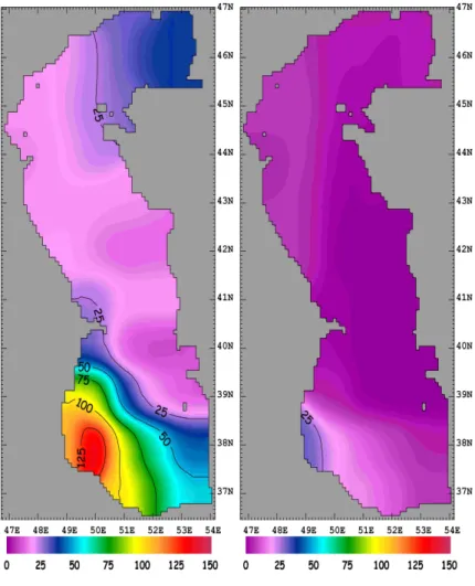
Winter mixing in the MCB and SCB is strongest in March and reaches 50–75 m depth in the interior regions of the MCB and 100–200 m along the shelf slopes (Fig. 13). Newly formed cold water with temperature of about 7–8◦C occupies the upper part of the basin interior, while the temperature is close to zero along the west coast.

Obser-20

vations of dissolved oxygen indicate large variations in the depth of convective mixing, depending on the bottom depth, location and the severity of winter. During moderate and mild winters, convective mixing is shown to reach depths of 150–200 m, as op-posed to severe winters when it reaches all the way to the bottom of the MCB (Baidin and Kosarev, 1986).

25

(22)

OSD

6, 1913–1970, 2009

Title Page

Tables Figures

◭ ◮

Back Close

Full Screen / Esc

Interactive Discussion (Fig. 14), when the NCB is totally covered by ice. Maximum ice thickness of more than

70 cm is reached in the beginning of March. Model simulated ice growth, i.e. features such as the start of ice formation, periods of maximum ice cover and thickness, etc. are in agreement with the available observations (Kosarev and Yablonskaya, 1994). On the other hand, comparison with climatologic data shows that the ice edge is often about

5

50 km more to the south than indicated by the model, often extending south along the eastern coast of the MCB in moderate winters such as 1982. A smaller ice covered area in the model as compared to the observations could be a result of (i) higher air temperature in the NCB obtained from ECMWF data compared to the climatology, (ii) modified heat capacity of the extremely shallow areas of the NCB, artificially made

10

deeper due to numerical stability considerations.

As surface waters start warming in March, the temperature difference between the shelf and the deep-sea regions start to decrease. In the beginning of April, after the melting of ice, the last cold water patch remains in the north-eastern part of NCB, undisturbed by the weak circulation in the region.

15

The average SST values are around 25–26◦C, 22–23◦C and 25◦C respectively in the interior regions of the NCB, MCB and SCB (Fig. 15). The surface waters in the shallow coastal regions of the SCB are often much warmer, especially along the eastern shelf, where the temperature approaches 30◦C and the salinity is increased by high rates of evaporation near the desert. Cold water with temperature of 14–16◦C appears along

20

the eastern shelf of the MCB, in the well-known upwelling region of the Caspian Sea, as a result of the surface drift directed away from the coast. Upwelling along the east coast is a quasi-permanent circulation feature of the warm season, supported by climatologic (Kosarev and Yablonskaya, 1994) and satellite (Sur et al., 1998) observations.

The sea surface salinity distribution in spring and summer is qualitatively similar to

25

(23)

OSD

6, 1913–1970, 2009

Title Page

Tables Figures

◭ ◮

Back Close

Full Screen / Esc

Interactive Discussion coastal waters (S=15.6 ppt) and the less saline interior waters (S=13.2 ppt). Noticeable

salinity changes occur along the western coast of MCB in August, when the coastal current is deflected from the west coast and therefore the southernmost penetration of low salinity waters is limited only to as far south as 42◦N.

The surface mixed layer thickness changes from 15–25 m on the western coast of

5

MCB and SCB to about 10 m on the eastern coast of MCB, with essentially a two-layer density stratification developing in summer. A temperature difference of 14◦C develops across the seasonal thermocline, with the density increasing from 1067 kg m−3in the upper layer to 1095 kg m−3at the bottom (Fig. 16).

4.2 Air-sea fluxes of heat and mass

10

In this section we focus our attention on the seasonal air-sea fluxes of heat and mois-ture at the air-sea interface. Our model development for the Caspian Sea is unique in many respects: Flux estimates in the past often have been based on bulk formulae using extremely non-uniform and coarse data sets. We implement a more rigorous, interactive flux estimation scheme making use of oceanic and atmospheric surface

15

properties respectively obtained from the Caspian Sea model and the ECMWF reanal-ysis atmospheric model relying on global data assimilation. A thermodynamic sea ice model is further used to modify the surface fluxes when ice is formed. The requirement for mass conservation is relaxed in the model to account for a non-zero water budget of the sea with respect to the river and surface volume fluxes.

20

Estimation of surface heat flux from bulk formulae using monthly mean values of sur-face wind speed, humidity, air and sea sursur-face temperature, has been shown to differ by less than 10% from computations using all samples by Esbensen and Reynolds (1981), and has been confirmed to have a ratio of 1.02–1.09 for different parts of the Caspian Sea by Panin (1987). We thus employ a correction factor of 1.09 for sensible and latent

25

(24)

OSD

6, 1913–1970, 2009

Title Page

Tables Figures

◭ ◮

Back Close

Full Screen / Esc

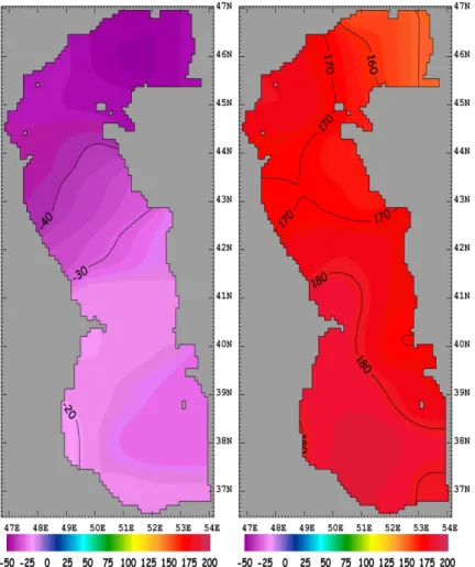
Interactive Discussion 4.2.1 Evaporation

In winter, a region of high evaporation in the eastern part of MCB (Fig. 17a) results from the combined effects of (i) cold and dry air intrusions from the eastern coast and (ii) warm water from the SCB advected along the eastern coast. The summer evapo-ration pattern is the opposite (Fig. 17b): the cold water along the eastern shelf of MCB

5

produces very little evaporation. Evaporation in summer has an increasing trend from north to south, except in the shallow NCB where evaporation is increased to almost twice the deep basin values. Analyses of monthly mean evaporation in the Caspian Sea made on the basis of 150 000 observations (Panin, 1987) are in good agreement with the simulated evaporation both in terms of distribution and magnitude. For

exam-10

ple, for the eastern part of MCB, Panin gives E=100–110 mm/month in January and E <40 mm/month in July, which are consistent with our estimates. On the other hand, Panin’s estimate ofE >180 mm/month in June–August in the southern part of the SCB is much higher than ours in the same region.

4.2.2 Sensible and latent heat fluxes

15

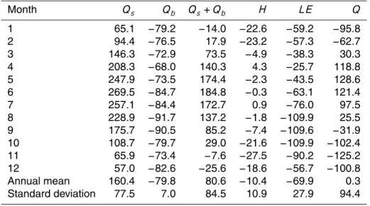
Monthly and annual mean heat budget components are given Table 1. In the annual mean budget, heat influx by solar radiation, amounting to 160.4 W/m2, is balanced by the outgoing thermal radiation (−79.8 W/m2), latent heat (−69.9 W/m2) and sensible heat (−10.4 W/m2) flux components.

The seasonal cycle of latent heat flux follows that of evaporation. In summer the

20

sensible heat flux almost vanishes as a result of the small difference between SST and air temperature. SST is higher than the air temperature in the NCB and SCB (Panin, 1987), while in the MCB, SST is usually lower than the air temperature as a consequence of upwelling. Sensible heat flux becomes relatively more significant in the heat budget in the autumn and winter seasons, when it is close to the net radiative

25

(25)

OSD

6, 1913–1970, 2009

Title Page

Tables Figures

◭ ◮

Back Close

Full Screen / Esc

Interactive Discussion In winter, the turbulent heat flux (sum of sensible and latent heat fluxes) at the sea

surface (Fig. 18a) has a maximum along the east coast of the MCB, produced by the interaction of the warm water tongue with overlying cold air (Figs. 5a and 12a). In this area both terms of the turbulent heat flux are of the same order (−250 W/m2for latent and−150 W/m2 for sensible heat flux), whereas in other parts of the sea, latent heat

5

flux is often 2–5 times larger than the sensible heat flux. In July (Fig. 18b), sensible heat flux in the same area decreases to about (−10)–(+20) W/m2and latent heat flux dominates in total flux.

4.3 Sea level variability and water budget

4.3.1 Mean sea level variability

10

Time series of model simulated and observed sea level anomaly at four Caspian Sea stations are shown in Fig. 19 for the year 1982. Station locations are shown in Fig. 20. Common features of the sea level time series at all four stations are the minimum in September–October, the rising trend from autumn to spring, followed by the fall in summer. There is a net rise in sea level at the end of the presented one year

pe-15

riod because the sea level is on a rising trend in the longer term. Good correlation in terms of amplitude and of phase between simulated and observed sea level demon-strates the model capability to reproduce key hydro- and thermo-dynamical processes of the Caspian Sea, of which the sea level is an integral measure. Root mean square difference between the simulated and observed curves changes from 1.4 cm at Baku

20

(26)

OSD

6, 1913–1970, 2009

Title Page

Tables Figures

◭ ◮

Back Close

Full Screen / Esc

Interactive Discussion 4.3.2 Spatial variability of the sea surface topography

The leading factors creating the observed spatial structure of sea surface topography in the model are baroclinicity and wind setup. Although the atmospheric forcing is variable in space and time, the following features emerge from a study of the seasonal cycle: (i) East-west asymmetry in buoyancy resulting from the distribution of fresh water

5

flux components (run-off, precipitation and evaporation). All major rivers enter the sea along the northwest coast. In the absence of other forcing, the fresh water introduced by the Volga River tends to flow along western coast, as a result of deflection by the Coriolis force. Precipitation and evaporation over the sea are extremely non-uniform. The southwest part of the SCB receives rainfall that is up to 10 times greater than the

10

other parts of the sea (Fig. 7), while the evaporation has somewhat smoother varia-tion over the basin. (ii) The predominant southward winds in the MCB and SCB are favourable for drifting surface water offthe eastern coast, thus producing typical coastal upwelling of cold and saline sub-surface waters along this coast. All of the above fac-tors support asymmetrical distribution of salinity, yielding high density waters on the

15

eastern shelf and relatively low density waters on the north and southwest parts of the sea, supporting the model produced west-east slope of the sea surface topography in Fig. 20. The spatial range of sea surface topography is minimum in July (7.5 cm) and maximum in December (15 cm), which is 2–3 times smaller then the seasonal range of sea level variations.

20

4.3.3 Water budget

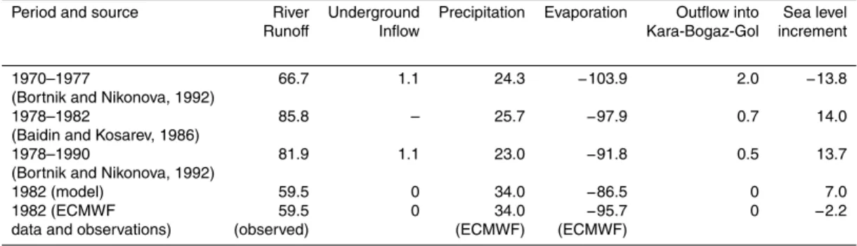
Estimates of Caspian Sea water balance terms based on various sources (Table 2) do not differ significantly from each other. The model simulated evaporation rate, of 86.5 cm/yr, is close to the estimate of Bortnik and Nikonova (1992) for the period 1978– 1990 and to the climatologic estimate of 96.3 cm/yr of Panin (1987).

25

(27)

OSD

6, 1913–1970, 2009

Title Page

Tables Figures

◭ ◮

Back Close

Full Screen / Esc

Interactive Discussion inter-annual variability of river runoff is extremely high. For example, the difference

between maximum and minimum yearly runoffin the last century is about 260 km3/yr or more than 100 cm/yr in terms of sea level rise (Bortnik et al., 1992).

Low river runoffin 1982 is compensated by high precipitation. The ECMWF reanaly-sis data for 1982 gives a value 28% higher than the estimates of Bortnik et al. (1992) for

5

the 1970–1977 and 1978–1990 periods. Precipitation in ECMWF reanalysis actually could have been underestimated, if one takes into account similar estimates elsewhere at around the same latitude, yielding 20% less precipitation compared to observations (Betts, Ball, and Viterbo, 1999).

Underground water flux into the sea is the least known component of the water

bal-10

ance, with different authors’ estimates in the range 0.3 to 49.3 km3/yr (Bortnik et al., 1992). As most estimates are relatively small, on the order of 3–5 km3/yr or about 1 cm/yr of mean sea level change, ground water inflow was not taken into considera-tion in the model.

In Table 2, we also give mean sea level increment estimated from observed river

15

runoffdata and precipitation/evaporation based on ECMWF reanalysis data. The dif-ference of 9.2 cm/yr between ECMWF estimated and observed sea level change gives a measure of error of the modern estimations of the water balance.

5 Sensitivity experiments

As already pointed out, the water budget of Caspian Sea is extremely sensitive to

20

climatic variability. In fact, the present sea level variations are much smaller than the contributing terms of river runoff, precipitation and evaporation, which tend to balance each other. Therefore, small differences in water budget components can lead to large changes in sea level. It is a widespread opinion that inter-annual variability of sea level is controlled by river runoffwhile anomalies of precipitation and evaporation have less

25

(28)

OSD

6, 1913–1970, 2009

Title Page

Tables Figures

◭ ◮

Back Close

Full Screen / Esc

Interactive Discussion A set of experiments was performed to ascertain the sensitivity of the circulation and

sea level change to external forcing and model parameters. We refer to the above ex-periment with the parameters and forcing given earlier, as the control run (CR). In the following experiments, we have run the model with further variations in model param-eters and of external forcing, using the beginning of the fourth year of the CR as initial

5

conditions.

In the first two experiments we examine the sea level change and circulation in re-sponse to variations in prescribed water budget components, i.e. river runoffand pre-cipitation. Next are the experiments with variations of atmospheric parameters, which determine the evaporative flux, i.e. the air and dew point temperature, and wind speed.

10

In further experiments we describe the sensitivity of the model to solar radiation and to parameterisation of the solar radiation penetration into the sea. In the last experiment, we analyse the sensitivity of the model to variations of vertical mixing. In most of these sensitivity experiments we have implemented external forcing, which varied from the central run comparable with the observed inter-annual variability in them. Seasonal

15

sea level changes derived from the sensitivity experiments are shown in Fig. 21. 5.1 Experiment 1: 50% increase in river runoff

We increase the runoffof all rivers by 50%. The reaction of the water budget and of sea level is quite expected and is almost linear. Mean sea level compared to the CR is increased by 28.3 cm/yr, corresponding to a value less than the 29.8 cm/yr that would

20

be obtained by linear extrapolation. The small non-linear response of the water budget is related to increased stability of the water column followed by an increase of SST, which leads to excessive evaporation compared to the CR. The main consequence of increased runoffon circulation is the extension of western coastal current towards the south.

(29)

OSD

6, 1913–1970, 2009

Title Page

Tables Figures

◭ ◮

Back Close

Full Screen / Esc

Interactive Discussion 5.2 Experiment 2: 50% increase in precipitation

Based on linear extrapolation we expect an increase of 17 cm/yr in sea level when precipitation is increased by 50% (Table 2), while the model gives an increase of 16.4 cm/yr. As in the first experiment, we have more stable water column especially in the SCB, due to excessive precipitation.

5

5.3 Experiment 3: 50% increase in wind speed

Much stronger non-linear reaction occurs in the case of increased wind speed. Based on linear extrapolation, the sea level would be expected to drop by 43.2 cm/yr, amount-ing to 50% increase in annual evaporation (Table 2). Because mixamount-ing is enhanced by increased wind stress, both the sensible and latent heat fluxes are affected, thus

con-10

siderably modifying the expected reaction. As cooling is increased, SST decreases by 1–2◦C compared to the CR, decreasing the surface humidity yielding a smaller spe-cific humidity difference at the sea surface and at 10 m height (qsurface−q10 m). The increased wind stress also changes the circulation. The overall decrease of mean sea level produced by the model is 13.0 cm/yr, which is about 3.3 times smaller than

15

expected from a proportional linear calculation. 5.4 Experimant 4: 5◦C warmer air temperature

When air temperature is warmer and the dew point temperature is the same as that used in CR, the obvious reaction of the model is an increase of SST (up to 2◦C in summer) and corresponding increase of specific humidity at the sea surface, resulting

20

(30)

OSD

6, 1913–1970, 2009

Title Page

Tables Figures

◭ ◮

Back Close

Full Screen / Esc

Interactive Discussion 5.5 Experiment 5: Warmer and more humid air

An increase of the dew point temperature by 5◦C compared to Experiment 4 affects the water balance in the opposite direction. Higher specific humidity of air prohibits the excessive evaporation observed in the previous experiment, leading to 6.2 cm/yr higher rise of sea level compared to the CR and of 19.6 cm/yr as compared to Experiment 4.

5

As a result of the restricted latent heat flux, the surface waters are warmer by 2◦C compared to Experiment 4.

5.6 Experiment 6: Solar radiation without correction

In the CR we have used ECMWF solar radiation heat flux with a correction factor of 1.05 to ensure better correspondence to climatologic estimates. The primary influence

10

of correction of solar radiation is on the SST. In the experiment without correction we have 1◦C lower SST compared to climatology, though the seasonal cycle of currents and of upper mixed layer show very little change. In response to the lower SST in the model we have lower evaporation, with an annual budget giving 5.7 cm/yr higher rise of sea level as compared to CR.

15

5.7 Experiment 7: Absorption of solar radiation at the sea surface

In this experiment we have checked the sensitivity of the seasonal cycle of sea level to parameterization of solar penetration into the sea. In Eq. (22) we put attenuation length for the short fraction of the solar radiation equal to 0.033 m, such that all the solar radiation is absorbed in the first model layer. Compared to the CR, SST starts to

20

increase much faster in the spring to produce a sharper thermocline and a shallower upper mixed layer. As a result, we have higher values of SST and of evaporation in the period from January till September. On the other hand, the balance between sen-sible and latent heat release from the sea is modified such that relatively larger part of the heat flux is accounted by sensible heat flux. In May, the sensible and latent

(31)

OSD

6, 1913–1970, 2009

Title Page

Tables Figures

◭ ◮

Back Close

Full Screen / Esc

Interactive Discussion heat fluxes are equal to (−10.8; −65.2) W/m2 compared to (−2.3; −43.5) W/m2 in the

CR, which means that the heat formerly released through evaporation or stored in the upper mixed layer is now released through sensible heat. In the period from Septem-ber till DecemSeptem-ber, the balance between sensible and latent heat fluxes is changed. In November we have (−19.0; −73.6) W/m2 for sensible and latent heat fluxes as

com-5

pared to (−27.5; −90.2) W/m2in the CR. The reduced penetration of heat into the sea results in stronger surface currents and more pronounced influence of baroclinicity on the circulation pattern.

5.8 Experiment 8: Constant vertical mixing coefficients

This experiment is designed to explore how the specification of mixing coefficients

10

modifies the circulation. We take constant values ofK_m andK_h, equal to the maximum values of (50.,10.)×10−4m2s−1 used in the CR. The reaction of the sea circulation is dramatic, sea currents become almost barotropic. The major effect of increased vertical mixing is a lowering of the SST by about 11◦C in August and a corresponding decrease of evaporation from the sea surface as compared to the CR. Annual sea level

15

rise is increased by 34.1 cm/yr compared to the CR. The fall of sea level in August-October typical of the seasonal cycle in the CR is now absent, due to insufficient heat stored in the summer.

6 Summary and conclusions

A coupled sea hydrodynamics – air/sea interaction – sea ice thermodynamics model

20

has been developed to simulate intra-annual variability of the Caspian Sea circulation and sea level. Complex bottom topography including large shallow areas, wide shelf and slope regions, interconnected sub-basins, large freshwater inflows, sensitive re-sponse to atmospheric forcing, sea ice formation, and the observed level of climatic variability combined with man-made changes in hydrology make the Caspian Sea a