www.atmos-chem-phys.net/15/685/2015/ doi:10.5194/acp-15-685-2015
© Author(s) 2015. CC Attribution 3.0 License.
Mercury vapor air–surface exchange measured by collocated
micrometeorological and enclosure methods – Part I: Data
comparability and method characteristics
W. Zhu1,2, J. Sommar1, C.-J. Lin1,3,4, and X. Feng1
1State Key Laboratory of Environmental Geochemistry, Institute of Geochemistry, Chinese Academy of Sciences, Guiyang 550002, China
2University of Chinese Academy of Sciences, Beijing 100049, China
3Department of Civil Engineering, Lamar University, Beaumont, TX 77710, USA
4College of Environment and Energy, South China University of Technology, Guangzhou 510006, China
Correspondence to:X. Feng ([email protected]) and J. Sommar ([email protected])
Received: 24 July 2014 – Published in Atmos. Chem. Phys. Discuss.: 1 September 2014 Revised: 15 December 2014 – Accepted: 17 December 2014 – Published: 19 January 2015
Abstract.Reliable quantification of air–biosphere exchange flux of elemental mercury vapor (Hg0)is crucial for under-standing the global biogeochemical cycle of mercury. How-ever, there has not been a standard analytical protocol for flux quantification, and little attention has been devoted to characterize the temporal variability and comparability of fluxes measured by different methods. In this study, we de-ployed a collocated set of micrometeorological (MM) and dynamic flux chamber (DFC) measurement systems to quan-tify Hg0flux over bare soil and low standing crop in an agri-cultural field. The techniques include relaxed eddy accumu-lation (REA), modified Bowen ratio (MBR), aerodynamic gradient (AGM) as well as dynamic flux chambers of tradi-tional (TDFC) and novel (NDFC) designs. The five systems and their measured fluxes were cross-examined with respect to magnitude, temporal trend and correlation with environ-mental variables.
Fluxes measured by the MM and DFC methods showed distinct temporal trends. The former exhibited a highly dy-namic temporal variability while the latter had much more gradual temporal features. The diurnal characteristics re-flected the difference in the fundamental processes driv-ing the measurements. The correlations between NDFC and TDFC fluxes and between MBR and AGM fluxes were sig-nificant (R>0.8,p<0.05), but the correlation between DFC and MM fluxes were from weak to moderate (R=0.1–0.5). Statistical analysis indicated that the median of turbulent
fluxes estimated by the three independent MM techniques were not significantly different. Cumulative flux measured by TDFC is considerably lower (42 % of AGM and 31 % of MBR fluxes) while those measured by NDFC, AGM and MBR were similar (<10 % difference). This suggests that incorporating an atmospheric turbulence property such as friction velocity for correcting the DFC-measured flux ef-fectively bridged the gap between the Hg0fluxes measured by enclosure and MM techniques. Cumulated flux measured by REA was∼60 % higher than the gradient-based fluxes. Environmental factors have different degrees of impacts on the fluxes observed by different techniques, possibly caused by the underlying assumptions specific to each individual method. Recommendations regarding the application of flux quantification methods were made based on the data obtained in this study.
1 Introduction
phase, Hg0 is prone to undergo hemispherical-scale tropo-spheric transport (Durnford et al., 2010). Hg0 is subject to bi-directional exchange between atmosphere and natural sur-faces through complex and yet not well understood processes (Bash, 2010; Gustin and Jaffe, 2010). Recent estimation indi-cates that annual natural emission accounts for two-thirds of global release of atmospheric Hg (Pirrone et al., 2010). How-ever, current estimates of natural exchange quantity remain highly uncertain due to the limitations in accuracy and repre-sentativeness of measurement techniques (Gustin and Jaffe, 2010; Pirrone et al., 2010).
There exist multiple experimental approaches to gauge Hg0 air–surface exchange, which can be grouped into en-closure and micrometeorological (MM) methods (Sommar et al., 2013a). Dynamic flux chambers (DFCs) representing the smallest scale, as the areas covered are typically in the order of 0.1 m2, are the most extensively applied method for quantifying Hg0evasion from and deposition to soil (Pois-sant and Casimir, 1998; Stamenkovic and Gustin, 2007; Xiao et al., 1991; Carpi and Lindberg, 1998). For measuring Hg0 fluxes on larger landscape scales, MM techniques represent an attractive alternative to DFCs. They allow spatially av-eraged measurements over a large area without disturbing ambient environmental conditions. For trace gases such as CO2, CH4, O3, NH3, HNO3, and selected volatile organic compounds (VOCs), eddy covariance (EC) is the preferred MM technique for quantifying air–landscape gas exchange (Aubinet et al., 2012; Farmer et al., 2006; Park et al., 2013; Whitehead et al., 2008). However, due to the lack of a suf-ficiently fast and sensitive sensor for the ultra-trace levels of Hg0in air, true EC measurement of background Hg0flux has not yet been accomplished. MM techniques applied in Hg0 flux (also called turbulent flux) quantification include the re-laxed eddy accumulation method (REA, also known as con-ditional sampling, CS) (Bash and Miller, 2008; Cobos and Baker, 2002; Olofsson et al., 2005; Sommar et al., 2013b), the aerodynamic gradient methods (AGMs) (Baya and Van Heyst, 2010; Cobbett and Van Heyst, 2007; Converse et al., 2010; Edwards et al., 2005; Fritsche et al., 2008a; Fritsche et al., 2008b; Marsik et al., 2005), and the modified Bowen ratio method (MBR) (Converse et al., 2010; Fritsche et al., 2008a; Fritsche et al., 2008b; Lindberg et al., 1995; Pois-sant et al., 2004). MM methods estimate turbulent transport with the assumptions of fetch homogeneity and the measure-ments are made within the constant flux layer (Wesely and Hicks, 2000). For example, REA-derived flux relies on ac-curate measurement of the concentration difference between upward and downward moving air parcels while gradient-derived flux is estimated from the vertical concentration gra-dient and the associated turbulent exchange parameters. For the traditional DFC (TDFC) methods, flux is derived from a steady-state mass balance over the chamber. More recently, we have designed and deployed a DFC of novel design (NDFC) based on surface wind shear condition (friction
ve-locity) rather than on artificial fixed flow to account for nat-ural shear conditions (Lin et al., 2012).
Limited efforts have been devoted to Hg0 flux measure-ment comparison. In the Nevada STORMS campaign (4-day duration), TDFCs and MM gradient methods were deployed to measure Hg0 flux over a heterogeneously Hg-enriched fetch. The TDFC- and MM-derived fluxes differed by one order of magnitude (Gustin et al., 1999; Gustin and Lind-berg, 2000; Poissant et al., 1999; Wallschläger et al., 1999). Subsequent investigations have suggested that TDFCs of dif-ferent sizes, shapes and operation flow rates yield difdif-ferent fluxes (Eckley et al., 2010; Lin et al., 2012; Zhang et al., 2002; Wallschläger et al., 1999). Gradient methods were de-ployed to measure seasonal Hg0fluxes over grasslands in the Alps (Fritsche et al., 2008b) and over a meadow in the Ap-palachians (Converse et al., 2010), the observed flux means varied by up to one order of magnitude. Collocated flux mea-surement using both MM and DFCs techniques for method evaluation and data synthesis remains scarce (Gustin, 2011). This limits a thorough comparison of flux data obtained by different techniques.
Measured fluxes are estimates of unknown quantities of air–surface exchange under field conditions and a reference technique for validating the estimates does not exist. Each available technique has its specific advantages and draw-backs and its applicability to obtain representative fluxes is limited under particular atmospheric conditions and site characteristics. It is therefore essential to compare and review uncertainties of the major techniques deployed for measur-ing air–ecosystem Hg0exchange. The objective of this study is to investigate the method characteristics, data comparabil-ity and measurement uncertainty of Hg0exchange fluxes as measured by five collocated MM and DFC methods includ-ing REA, MBR, AGM, TDFC and NDFC. We improved a number of measurement platforms (Lin et al., 2012; Sommar et al., 2013b) and performed two intensive field campaigns over both bare and vegetated landscapes. The results of this integrated assessment are presented in part by two compan-ion papers. In Part I, we evaluate the technical merits of the examined flux quantification methods, assess the flux vari-ability and data comparvari-ability, and address the method ap-plicability under a given set of environmental conditions. In Part II, we quantify the bias and uncertainty of the examined flux measurement methods.
2 Material and methods 2.1 Flux measurement methods
2.1.1 Dynamic flux chamber techniques
of 0.06 m2has been used extensively in our group and else-where (Feng et al., 2005; Fu et al., 2008, 2010, 2012; Li et al., 2010; Wang et al., 2005, 2007; Zhu et al., 2013a). The NDFC was fabricated of thin polycarbonate sections and enclosed a soil surface of 0.09 m2(for details, see Lin et al., 2012). The NDFC internal flow condition was precisely controlled to relate to the applied flushing flow rate to the atmospheric boundary shear condition (therefore wind shear condition) and the calculated flux was re-scaled to boundary shear con-dition (Eq. 2 below). Both DFCs were operated at a relatively high flushing flow rate of 15 L min−1, corresponding to turn-over times (TOTs) of 0.32 min and 0.47 min for TDFC and NDFC, respectively. The flux from TDFC and NDFC were calculated following Eq. (1) and (2), respectively (Xiao et al., 1991; Lin et al., 2012):
FHgTDFC0 =
Q(Co−Ci)
A (1)
FHgNDFC0 =
Q(1C) A
kmass(a) kmass(m)
(2)
=Q(Co−Ci)
A
4.86+ 0.03(h/ l)[hu∗/(6kz0)](DH/D) 1+0.016{(h/ l)[hu∗/(6kz0)](DH/D)}2/3
4.86+1+00.03(h/ l)(Q/Ac)(DH/D)
.016[(h/ l)(Q/Ac)(DH/D)]2/3
,
whereFHgTDFC0 is Hg0flux measured from the TDFC method,
FHgNDFC0 is Hg0flux from the NDFC method,Qis applied flow
rate (0.9 m3h−1),Ais footprint (0.06 m2for TDFC, 0.09 m2 for NDFC), Co and Ci are the DFC outlet and inlet air Hg0concentration, andkmass
(a)andkmass(m) are the overall mass transfer coefficient (m s−1)in the near-surface bound-ary layer and in the internal layer within NDFC, respec-tively.Acis the NDFC flow cross-sectional area (0.009 m2), l is the distance measured from the starting point of the measurement zone (0.15 m),his the height of NDFC (0.03 m), u∗ is the atmospheric boundary layer friction velocity,
andz0 is surface roughness height (m).DH andD are the NDFC hydraulic radius (0.0545 m) and diffusivity of Hg0 (1.194×10⁻⁵m2s−1), respectively.
2.1.2 Micrometeorological techniques Relaxed eddy accumulation (REA) method
A REA system of whole-air type was deployed with the de-sign and operation parameters described elsewhere (Sommar et al., 2013b; Zhu et al., 2013b). The REA apparatus con-stitutes of open path EC (OPEC) and conditional gas sam-pling system. The OPEC part included a 3-D fast-response anemometer, an open path CO2/H2O analyzer, and a micro-logger with processing and control capabilities. MM data collected at 10 Hz are acquired and processed by the lat-ter, which also control the execution of conditional sampling valves from its 12 V terminal following the implemented dy-namic wind dead-band algorithm to accurately isolate
up-and down-drafts present in sampled turbulent air parcels. Turbulent REA flux was computed according to
FHgREA0 =βsσw
C↑−C↓
| {z }
1CREA
=βsσw (
X
i
m↑i ti·Q↑i ·α
↑
i
−X
i
m↓i ti·Q↓i ·α
↓
i )
, (3)
whereσw(m s−1)is the standard deviation of vertical wind speed (m s−1)andC↑/↓is the concentration of Hg0(at stan-dard temperature and pressure) for the up- and down-moving eddies corrected for dilution of zero air injection, respec-tively (ng m−3). The operational form of Eq. (3) is given in the right-hand side, in which, for samplei,m↑i/↓is the mass of Hg0 derived for the up- or down-draft channels (pg), ti is the total duration (min),Q↑i/↓is the continuous flow rate through the up- or down-draft channels (L dry air min−1), andα↑i/↓is the fraction of time the up- or down-draft condi-tional sample valves are activated.βs is a dimensionless re-laxation coefficient (calculated from scalars)which for each averaging period (20 min) was calculated on-line from suit-able scalarsthose fluxes (FsEC=ρd·w′χs′) can be measured by the OPEC system (in addition to CO2flux, buoyancy flux CP·w′Ts′and for latent heat fluxλ·w′q′, symbol definitions see appendix in Sommar et al., 2013b) as well as by REA according to
βs=w′χs′ . h
σw
χs↑−χs↓ i
, (4)
whereχs↑/↓is the mixing ratio of the specific scalar quantity for the up- and downdraft (kg kg−1).
Aerodynamic gradient micrometeorological (AGM) method
The AGM method is based on an analogy application of Fick’s first law stating that turbulent bi-directional flux of a scalar from surface (FAGM
two heights, the flux can be expressed as
FHgAGM0 = −KH(u∗, ς )
∂C ∂z
= − κu∗
lnz2−d z1−d
−ψH(ς2)+ψH(ς1)
| {z }
υtr
· CZ2−CZ1
| {z }
1C
, (5)
whereκ is von Kármán constant (∼0.41),u∗ is the friction velocity (m s−1), theυtrterm is the transfer velocity (m s−1), z2 andz1are the heights of the upper and lower sampling inlet (m), andψHis the integrated universal function for sen-sible heat to correct for deviations from the ideal logarithmic profile.ψH is parameterized as a function ofςm (ς1andς2 represent the parameter at z2 andz1 respectively), and fur-thermoreCZ2 andCZ1 are the Hg0 concentration (ng m−3)
atz2andz1, respectively.
Modified Bowen ratio (MBR) method
The MBR method assumes that the flux of a trace gas can be related to that of a surrogate scalar determined from OPEC measurements (e.g., sensible and latent heat, CO2 flux, and H2O flux) (Converse et al., 2010; Lindberg et al., 1995). In this study, temperature was used as the proxy scalar, which was monitored at the heights coinciding with measurement of Hg0 concentration. The Hg0flux is calculated following Walker et al. (2006):
FHgMBR0 =w′T′·
C(z2)−C(z1) T (z2)−T (z1)=w
′T′·1C
1T, (6)
whereFHgMBR0 is the Hg0flux (ng m−2h−1)measured with the MBR method, w′T′ is kinematic heat flux (K m s−1) mea-sured by EC, while1Cand1T are the vertical gradients of Hg0concentration (ng m−3)and air temperature (K), respec-tively. The ratio w′T′/1T is known as the eddy diffusivity
for heat.
2.2 Site description and sampling
The flux measurement experiments were conducted at Yucheng Comprehensive Experimental Station, Chinese Academy of Sciences (36◦57′N, 116◦36′E), which is a
semi-rural agricultural station located in the North China Plain approximately 50 km from Jinan, Shandong Province. Within a radius of ∼5 km the planting system is winter
wheat (Triticum aestivum Linn., November–May) or
sum-mer maize (Zea mays, June–October) for a rotation in a year.
The surface soil texture in this area is silty loam consisting of 12 % sand, 22 % clay and 66 % silt with moderate salin-ity and alkalinsalin-ity (pH=8.6) (Hou et al., 2012). The agri-cultural fields adjacent to the sampling site are relatively flat (level differences < 1.5 m within 1 km) and the total Hg content in surface soil is spatial homogeneously distributed
(45±3.9 µg kg−1,n=27) (Zhu et al., 2015a). Two intensive
field campaigns were performed: one in late autumn 2012 (IC#1, 4–24 November, DOY (day of year) 309–329) and the other in spring 2013 (IC#2, 16–25 April, DOY 106–115). IC#1 was carried out over the ploughed bare soil surface us-ing AGM, MBR, TDFC, and NDFC. IC#2 was carried out over wheat canopy (average height ∼0.36 m, leaf area in-dex of 3.4) using REA, AGM and MBR. Given the tight row spacing of the grain field, the deployment of DFCs was not permissible during IC#2.
2.3 Instrumentation
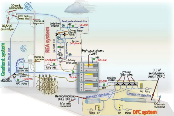
A 6.5 m MM flux tower was installed at the same location for both campaigns (Fig. 1). The instrumentation system consists of the tower-based MM systems and ground-based DFCs. The OPEC system consisted of a Campbell CSAT-3 sonic anemometer–thermometer, Licor LI-COR 7500A open-path CO2/H2O analyzer and HMP155A humidity–temperature sensors, a standard instrumentation combination used in long-term ecosystem instrumentation networks (Mauder et al., 2013). REA sampling inlet was positioned at 2.96 m above ground. By using a set of 2/3-way automated mag-netic switching unit (Tekran® 1110) coupled with an auto-mated Tekran®2537B Hg vapor analyzer operated at a flow rate of 0.75 L min−1, up- and down-draft conditional samples were sequentially routed into the analyzer at 10 min intervals (two 5 min samples). For gradient measurements, the temper-ature and relative humidity sensor (HMP155A, Vaisala Oy, Finland) housed in radiation shields and corresponding Hg0 intake was assembled at two heights of 2.96 m and 0.76 m. The two-level Hg0 vertical gradient profiling system con-sisted of two separate inlet lines (PFA Teflon), each with an inlet filter (0.2 µm PFA Teflon), were routed to another sampling manifold (Model 1110). Another Hg0gas analyzer (Model 2537B) is connected to the outlet of the manifold and the profile inlets are opened one at a time synchronized with 2537B’s sampling cycles. The manifold was configured to al-low the inlet not in use to be continually flushed by a bypass pump. Both the pump and 2537B are operated at a flow rate of 1.0 L min−1. An estimate of the vertical Hg0concentration gradient was derived every 20 min from measurements of the two heights sequentially, 5 min integrated samples.
Figure 1.Schematic illustration of the collocated MM and DFCs instrumentation set-ups. P, MFC and FM indicate a pressure transmitter, mass flow controller and flow meter of rotameter type respectively.
2.4 Quality assurance/control (QA/QC), data evaluation and EC flux corrections
The three Tekran®2537B analyzers (Fig. 1) were operated and maintained following the standard operation procedures of NADP (2011). The analyzers were regularly calibrated in the laboratory by manual injections of known amount of Hg0. The yielded recovery was 98–101 %. In the field, in-struments were calibrated every 48 h using the internal Hg0 permeation source. A soda-lime trap and a 0.2 µm Teflon membrane filter were located upstream of the inlet of all an-alyzers. The analyzers are sensitive to insufficient power and were therefore always supplied with grid power passing a 10 kW voltage stabilizer to ensure proper operation in the field. All the tubing and system valve blanks were checked before and after the campaigns by flushing with zero air ob-tained from a zero-air generator (Tekran®1100). Before the field measurement, the accuracy of two HMP 155A sensors was evaluated after periods of side-by-side measurements. The two DFCs were cleaned by 10 % HNO3and Milli-Q wa-ter prior to field deployment. Chamber blanks performed at the field site were consistently low for both DFCs (TDFC: 0.2±0.1 ng m−2h−1,n=19; NDFC: 0.3±0.2 ng m−2h−1, n=32) and not subtracted upon calculation of fluxes.
The REA-system enabled a mode during which air is sam-pled synchronously with both conditional inlets. This ref-erence mode provides an automated QC-measure to regu-larly check for gas sampling path bias, while the
gradient-based MM techniques require manual testing by collocat-ing gas samplcollocat-ing inlets and sensors. Such side-by-side tests were performed before or after a campaign. Post-processing of collected 10 Hz EC raw data was performed for each of the 20 min flux averaging periods using EddyproTM5.0 flux analysis software package (LI-COR Biosciences Inc.). A se-ries of standard data corrections were implemented follow-ing Sommar et al. (2013b) includfollow-ing the Webb–Pearman– Leuning (WPL) correction. Moreover, tests were applied on 20 min fast time (10 Hz) series raw data to qualitatively as-sess turbulence for the assumptions required of applying MM methods (steady-state conditions and the fulfillment of simi-larity conditions). The basic flag system of Mauder and Fo-ken (2004) was utilized to indicate limitation in turbulence mixing, quality indices of 0, 1 and 2 denoting high, moderate and low quality.
2.5 Meteorological data
Supporting meteorological data (sampled at 1 Hz and stored as 20 min averages) including relative humidity (RH, %), canopy leaf wetness (%), air temperature (◦C), event-based
rainfall (mm), wind speed (m s−1), wind direction (◦), solar
radiation (W m−2), soil temperature (◦C) and soil moisture
Figure 2.General meteorological parameters and ambient GEM concentration in the two campaigns. Upper panel: relative humidity (blue open circles), canopy leaf wetness (light blue line filled down), air temperature (red filled diamonds) and rainfall (black bar). Middle panel: wind speed (green line) and wind direction (dark green open circles filled down). Lower panel: ambient GEM concentration (dark purple open circles), global radiation (orange squares filled down) andσw/ u∗(magenta line).
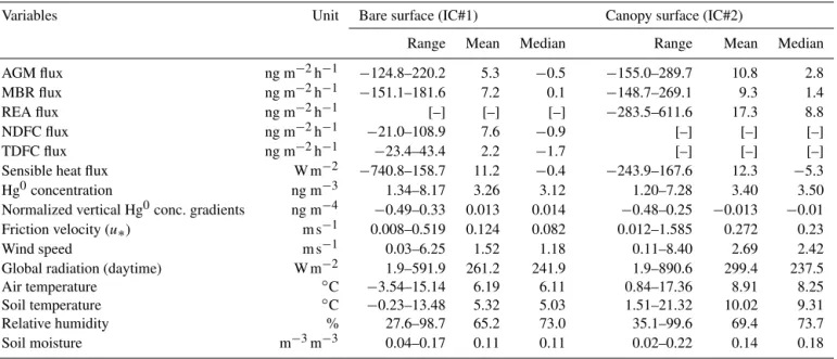
Table 1.Summary of observed meteorological variables, Hg0concentrations, vertical Hg0concentration gradients and Hg0fluxes for two campaigns.
Variables Unit Bare surface (IC#1) Canopy surface (IC#2)
Range Mean Median Range Mean Median
AGM flux ng m−2h−1 −124.8–220.2 5.3 −0.5 −155.0–289.7 10.8 2.8
MBR flux ng m−2h−1 −151.1–181.6 7.2 0.1 −148.7–269.1 9.3 1.4
REA flux ng m−2h−1 [–] [–] [–] −283.5–611.6 17.3 8.8
NDFC flux ng m−2h−1 −21.0–108.9 7.6 −0.9 [–] [–] [–]
TDFC flux ng m−2h−1 −23.4–43.4 2.2 −1.7 [–] [–] [–]
Sensible heat flux W m−2 −740.8–158.7 11.2 −0.4 −243.9–167.6 12.3 −5.3
Hg0concentration ng m−3 1.34–8.17 3.26 3.12 1.20–7.28 3.40 3.50
Normalized vertical Hg0conc. gradients ng m−4 −0.49–0.33 0.013 0.014 −0.48–0.25 −0.013 −0.01
Friction velocity (u∗) m s−1 0.008–0.519 0.124 0.082 0.012–1.585 0.272 0.23
Wind speed m s−1 0.03–6.25 1.52 1.18 0.11–8.40 2.69 2.42
Global radiation (daytime) W m−2 1.9–591.9 261.2 241.9 1.9–890.6 299.4 237.5
Air temperature ◦C −3.54–15.14 6.19 6.11 0.84–17.36 8.91 8.25
Soil temperature ◦C −0.23–13.48 5.32 5.03 1.51–21.32 10.02 9.31
Relative humidity % 27.6–98.7 65.2 73.0 35.1–99.6 69.4 73.7
3 Results and discussion 3.1 Meteorological conditions
Meteorological observations and ambient Hg0concentration during the two campaigns are presented in Fig. 2 and sum-marized in Table 1. The weather was predominantly sunny and temperate (−3.5 to 15.1◦during IC #1 and 0.8 to 17.4◦
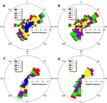
during IC#2). A rain shower yielding 3.4 mm precipitation occurred during IC#1. No precipitation was recorded dur-ing IC#2 (Fig. 2 upper panel). Leaf wetness and RH dis-played clear diurnal variation (RH dropped to 40 % and leaf wetness to 0 % during daytime) except during the precip-itation event when both were near saturation. Due to the high RH and sometimes sub-zero temperature at night, the ground and wheat possessed intermittently a light frost cover in early morning time. The wind speed was relatively high during daytime and turned moderate/calm at night. The wind direction was more variable from south to northeast with an average wind speed at 1.52 m s−1 (daytime mean: 1.98 m s−1, nighttime mean: 1.05 m s−1)in IC#1, and changed to southwest and northeast with a mean of 2.69 m s−1(daytime mean: 3.34 m s−1, nighttime mean: 1.97 m s−1)in IC#2. The wind directions in IC#2 were more consistent than in IC#1:
∼60 % of 20 min wind observations were of southwesterly
directions (Fig. 3a, c). The integral turbulence characteris-tics are indicated by σw/u∗ (Panofsky and Dutton, 1984). For neutral stratification, this ratio is approximately constant at 1.13–1.35 (Nemitz et al., 2009). The median σw/u∗ was
1.28 and 1.24 during IC#1 and IC#2. However, the variabil-ity introduced by diabatic condition is comparatively more pronounced during IC#1. Hg0observations at the sampling site showed a wide range of 1.20 to 8.17 ng m−3 (medians 3.12 ng m−3and 3.50 ng m−3during IC#1 and IC#2, respec-tively). The medians were elevated compared to the hemi-spheric background (1.5–1.7 ng m−3), but nevertheless ap-peared representative of a semi-rural area of North China plain (∼3.2 ng m−3, Zhang et al., 2013). The angular
distri-bution of Hg0observations (Fig. 3b, d) indicated a weak Hg0 concentration dependence on wind direction during IC#1 but a more manifest dependence appeared during IC#2, with el-evated concentrations associated with southerly and south-westerly winds (4.04–4.88 ng m−3, 45–130 % higher than those associated with easterlies, 2.12–2.79 ng m−3).
3.2 Hg0fluxes observed by the DFC techniques 3.2.1 Characteristics of DFCs Hg0fluxes
Descriptive statistics of the DFC Hg0flux observations are presented in Table 1. In a comparison, NDFC-derived Hg0 fluxes spanned over a broader range and exhibited a higher mean. Figure 4a displays the time series of Hg0fluxes gauged by the two DFC methods. Both series showed similar di-urnal features with daytime evasion (maximum occurred at
Figure 3.Polar histograms of 20 min averaged wind speed (m s−1) and Hg0 concentration (ng m−3):(a)wind rose during IC#1;(b) Hg0concentration rose during IC#1;(c)wind rose during IC#2;(d) Hg0concentration rose during IC#2.
midday) and a shallow minimum of bi-directional exchange during nighttime. The pattern is consistent with observations made over background soils worldwide (Gustin et al., 2011 and the references therein).
The median±MAD (median absolute deviation) of Hg0
flux was −0.9±3.2 and −1.7±4.3 ng m−2h−1 for TDFC
and NDFC, respectively. Probability plots of both DFC data sets showed positive kurtosis (3.0 and 4.1) and skewness (1.6 and 2.1) (Fig. 5) as a consequence of stronger emission and increased friction velocity at daytime. The substantial frac-tion of NDFC data points elevated in magnitude outlying the 1.5·IQR (interquartile range) bound is associated with peri-ods of high wind speed (i.e., showing the dependence of fric-tion velocity in Eq. 2). Moreover, as indicated in Fig. 5, the shortest half (50 %) of the chamber flux data is positioned more towards dry deposition for the novel compared to the traditional chamber technique. Nevertheless, the intrinsic di-vergence of the microenvironment inside enclosures in rela-tion to that of near-surface air layer tends to promote efflux.
3.2.2 Comparison of Hg0fluxes obtained from DFCs measurement
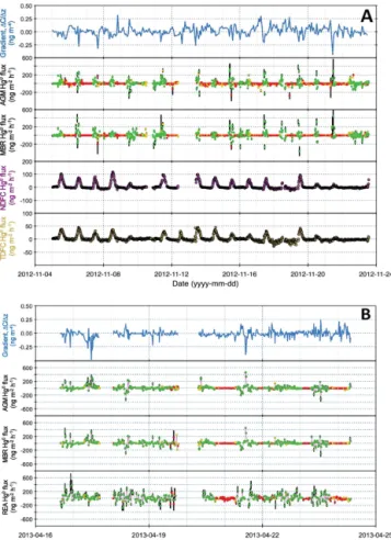
Figure 4. Time series of GEM gradients, GEM fluxes measured in:(a)IC#1 using MM and DFCs techniques;(b)IC#2 using MM techniques. The color code (green–yellow–red) denotes the quality (high–moderate–low) of turbulent flux data derived from general tests and black bars given in corresponding plots represent absolute flux uncertainties.
1999; Gustin and Lindberg, 2000). The observed difference was partially attributed to the substrate heterogeneity with re-spect to Hg content. In this study, the surface soil Hg content within the methodological footprint range is at large homo-geneous and therefore does not pose an interfering factor.
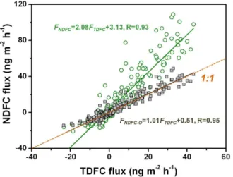
Eckley et al. (2010) examined experimentally a series of operational and instrumental factors that may influence DFC-derived flux. The DFC flushing flow rate was identified to have substantial positive influence. In the present study, the TOT of TDFC is 50 % smaller than that of the NDFC. More-over, the footprint of the traditional type is about two-thirds of the NDFC footprint and therefore a higher flux is expected using the NDFC method (Eckley et al., 2010; Lin et al., 2012). Figure 6 shows a scatterplot of the fluxes measured by the NDFC and TDFC approach before and after turbu-lence correction. The data were significantly positive corre-lated (R=0.93,R=0.95 between TDFC and NDFC fluxes calculated with Eq. (2) and Eq. (1) respectively; p<0.01). Quantitatively, direct measured flux was consistent for the
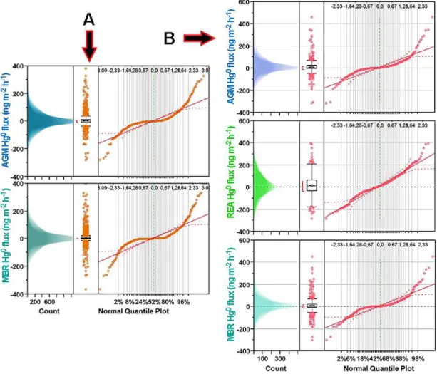
Figure 5.Distributions of Hg0 flux derived from DFC measure-ments (upper panel: TDFC, lower panel: NDFC). The tripartite pan-els consists from left to right of a shadowgram (a suite of overlaid histograms with different bin widths), a box and whisker plot (the ends of the box represent Q1 and Q3 and the whiskers denote±1.5 times the interquartile range, IQR=Q3−Q1; sample points further away are given as individual markers) and the corresponding normal quantile plot (the unbroken solid line signifies the expected nor-mal cumulative distribution and the dashed intervals the Lilliefors confidence bounds. The scale of the upper and lower abscissa in-dicates normal quantile and probability). Furthermore, in the box and whiskers plot, mean is indicated by a filled diamond while the median is the line within the box. The bracket outside of the box identifies the shortest half, which is the most dense 50 % of the ob-servations.
Figure 6.Scatterplot of Hg0flux obtained from TDFC and NDFC measurement (green open circles), and the NDFC calculated using Eq. (1) versus TDFC flux (gray filled squares).
3.3 Hg0fluxes inferred from MM methods
3.3.1 Characteristics of turbulent Hg0fluxes observed by micrometeorological methods
Figure 4a and b show the time series of normalized ver-tical Hg0 concentration gradient (ng m−4) and Hg0 flux (ng m−2h−1)derived from the turbulent diffusion methods (MBR and AGM). Hg0 concentration gradients were ob-served in the similar ranges of−0.49 to 0.33 and−0.48 to
0.25 ng m−4in both campaigns (Table 1 and Fig. 4), though the more occasionally shifting conditions of weak and de-veloped turbulence in IC#1 tend towards promoting a higher scale of diurnal gradient variability (IC#1 vs. IC#2 stan-dard deviation: 0.09 vs. 0.06). Our gradient observations are in alignment with measurement over temperate grasslands (−0.40 to 0.27 ng m−4)(Fritsche et al., 2008b).
Basic statistics of the MM Hg0 flux observations is pre-sented in Table 1. The variability in our observations is sim-ilar with those reported from previous studies using the MM flux measurement technique over uncontaminated croplands (corn, soybean and rice paddy fields) (Baya and Van Heyst, 2010; Cobos and Baker, 2002; Kim et al., 2003; Cobbett and Van Heyst, 2007). The MM fluxes exhibited strong tempo-ral variability during daytime and much weaker variability under low-quality turbulence during nighttime. In a typical campaign day, the turbulent flux data sets included both pe-riods of emission and dry deposition. The median of night-time flux was much smaller than the daynight-time flux for all MM methods (Mann–WhitneyUtest, MBR and AGMp<0.001, p<0.10 for REA).
The distribution of the turbulent fluxes and Hg0 con-centration gradient in Fig. 4 deviated significantly from a Gaussian distribution in the Hg0concentration gradient and in the derived MBR and AGM fluxes (Shapiro–Wilk’s test
rejected the hypothesis of normality of the distributions, p<0.01). The statistical MM fluxes (median ±MAD) in
IC#1 (Fig. 7a) were−0.5±8.9 and 0.1±3.2 ng m−2h−1for
AGM and MBR measurement, and 2.8±29.0, 1.4±15.2, and 8.8±45.3 ng m−2h−1for AGM, MBR and REA in IC#2 (Fig. 7b), respectively. All the distributions of MM turbu-lent flux were associated with a positive kurtosis (3.8–16.2) and a slightly positive skewness (0.8–1.5). The observed flux frequency distributions for AGM and MBR peaked more strongly than that of REA (Fig. 7), with the MBR method giving the most confined distribution. Broader flux distri-bution measured by the REA sampling method has been reported in the measurements of turbulent fluxes for other gases (Fowler et al., 1995; Beverland et al., 1996; Nemitz et al., 2001). Previous studies suggest that vegetation canopy in the growing stage acts as an Hg0 sink by net uptake of Hg0into foliage and therefore contributes to dry depositional flux (Bash and Miller, 2009; Stamenkovic and Gustin, 2007). However, the three MM techniques in this study derived sig-nificant higher average Hg0emission fluxes in IC #2 com-pared to IC#1, indicating that the vegetation sink strength was not sufficient to offset the efflux from underlying soil surface for croplands. Even though not measured, it is cred-ible to assume that the soil Hg0efflux was higher during the warmer IC#2 due to higher temperature (Table 1) (Baya and Van Heyst, 2010; Gustin, 2011).
3.3.2 Comparison of Hg0fluxes derived from micrometeorological methods
The larger variability in REA- compared to the gradient-derived fluxes is associated with a combination of method-ological, instrumental and site-specific constraints influenc-ing primarily the resolution of 1CREA (Eq. 3) as identi-fied and discussed in Part II of this paper series (Zhu et al., 2015b). Nevertheless, a Friedman two-way analysis of variance by ranks (a non-parametric method) showed that the median fluxes by the three MM methods were not sig-nificantly different (χ2=1.29< χ2
p=0.05=5.99). This indi-cated that AGM, MBR and REA methods produced compa-rable results with respect to the median location of Hg0 tur-bulent flux during the inter-comparison.
pro-Figure 7.Overview of the distributions of turbulent Hg0flux measured by the MM techniques:(a)IC#1,(b)IC#2. See Fig. 5 for a detailed description of the composite plots.
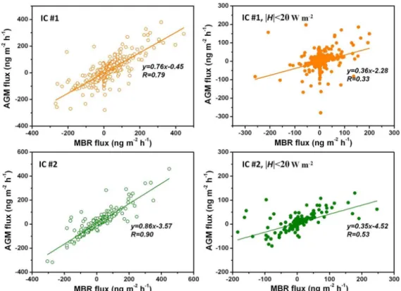
cess (see Sect. 3.4). The MBR method becomes uncertain and may significantly overestimate flux when the numera-tor and denominanumera-tor in the formula of eddy diffusivity ap-proach small numbers, which typically occurs in periods at dawn, dusk and during nighttime (Eq. 6, see Converse et al., 2010). As shown in Fig. 8, the 20-min-averaged AGM- and MBR-derived fluxes were well correlated during both cam-paigns (slopes of 0.76 and 0.86). However, when the sensi-ble heat flux becomes small (small temperature gradient) at
|H|<20 w m−2, the correlation coefficient diminishes dras-tically with a fall-off in slope (FAGM/FMBR=0.35–0.36) implying that the MBR method can significant overestimate turbulent Hg0 fluxes. MBR flux data collected in the pres-ence of small scalar gradients (often during dawn and dusk transition periods) are therefore of questionable quality and should be considered for omission.
AGM fluxes were on an average 26.1 % lower than MBR fluxes during IC #1, but 13.8 % higher during IC#2. The disparate results may largely stem from methodological is-sues (Fritsche et al., 2008b). In some previous studies us-ing the AGM method to gauge various trace gas fluxes
in-cluding Hg0 (Edwards et al., 2001; Edwards et al., 2005; Simpson et al., 1997), normalization of Eq. (5) was intro-duced to mitigate for systematical failure of obtaining en-ergy budget closures (Twine et al., 2000) by a factor of 1.3– 1.35. The AGM method involves momentum flux, and an at-mospheric stability parameterization in the flux calculation. For the conditions of weak developed turbulence to a greater extent prevailing under nocturnal stable stratification, where u∗ is very low, the AGM and MBR methods are prone to
large uncertainties and corresponding fluxes are suggested to be flagged by applying wind or friction velocity thresholds (namelyu∗<0.07–0.1 m s−1) (Fritsche et al., 2008b; Foken,
Figure 8.Scatterplots of 20 min MBR versus AGM flux during IC#1 (upper panel) and IC#2 (lower panel). The plots on the right-hand side depict specific data for which|H|<20 w m−2.
variability in REA flux is generically observed (Nemitz et al., 2001; Fowler et al., 1995; Moncrieff et al., 1998). In addition, systematic flux differences between a suite of NH3-REA sys-tems as well as collocated AGM system inter-compared have been reported (Hensen et al., 2009).
3.4 Comparison of chamber and micrometeorological techniques
3.4.1 Footprint of flux measurement
While the footprint (enclosed soil surface) of the chamber methods is fixed and very small (0.06 m2 for TDFC and 0.09 m2for NDFC), MM methods derive fluxes from a foot-print of comparatively large spatial extension upwind of the sampling tower. The MM footprint is not constant over time but a complex function of the sensor height, surface rough-ness length and canopy structure together with changing me-teorological conditions. The predicted source area (using the models of Kljun et al., 2004 and Kormann and Meixner, 2001) tends for upper sampling level (z2=zREA) to be ex-tensive for flux periods associated with weakly developed turbulence (Flag 2). In contrast, ∼70 % and∼86 % of the
data cleared for good turbulence quality, xˆ70% (along-wind distance providing 70 % cumulative contribution to turbulent flux) fall within the unbroken field (150 m) for IC#1 and IC#2 respectively. For the lower sampling height (z1), the footprint falls almost entirely within the primary fetch. Nevertheless, heterogeneous structures (roads, streams, tree stands and low buildings) existing outside the primary fetch (> 150 m) are of minor spatial extent, and within a radius of∼2 km the
sam-pling tower can be regarded to be surrounded by unbroken farmlands.
3.4.2 Diel variations
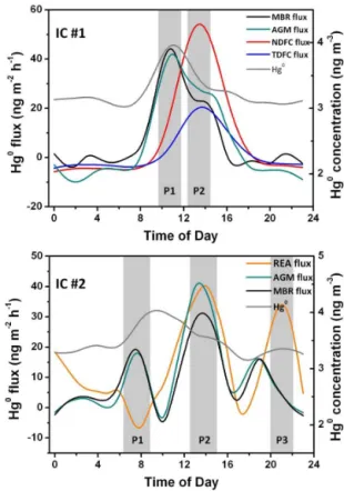
Figure 9 shows box and whisker plots of the diurnal vari-ation of Hg0 flux obtained by the five examined methods. Consistent in both campaigns, the MM methods exhibited highly variable fluxes, especially during daytime, where the magnitude in a single 20 min turbulent flux can exceed the flux derived by the chamber methods by many times. DFCs fluxes followed a well-defined diurnal pattern with consistent daytime emission and slight nighttime deposition. The pat-tern is similar to those for solar irradiance and temperature and reflects that the air–soil Hg0flux derived from the DFC technique is primarily governed by thermal and light-induced controls (e.g., Bahlmann et al., 2006). In contrast, flux from MM measurements is subject to the constant changes of at-mospheric turbulence within the planetary boundary layer. To facilitate a comparison between the DFC and MM data set on a diurnal basis, a Savitzky–Golay filter was applied on hourly averaged turbulent Hg0 flux data to smooth out the short-term variability. In Fig. 10, where the diurnal courses of flux are given by smoothing spline fits, there is a 2 h lag
Figure 10.Smoothed diurnal cycles of Hg0flux and Hg0 concen-tration derived from hourly averaged input data.
in the time of the day when turbulent and chamber-derived flux peaked (IC#1). For the DFCs, the observed Hg0 flux peaked within the period P2 (Fig. 10, IC#1) in concert with soil temperature, which is consistent with diurnal cycles re-ported for chamber measurements in the literature (Fu et al., 2008, 2012; Gustin, 2011; Zhu et al., 2013a).
some importance. However, to fully quantify the advection term for Hg0 requires an array of instrumentation and such an investigation was not feasible in this study.
The mean diurnal cycles calculated for the three coevally examined MM methods (Fig. 10, IC#2) are based on a sig-nificantly smaller set of input data (∼30 % of IC#1) and therefore plausibly less robust to provide adequate repre-sentativeness after smoothing. Moreover, the campaign is a composite of periods where near-neutral conditions pre-vailed on daytime as well as adjacent nights and periods with weakly developed turbulence during nighttime respectively. Accordingly, the MM methods unanimously gauged maxi-mum fluxes slightly after noon-time (P2, IC#2). However, there are features (P1 and P3) in the constructed cycles that are difficult to fully couple to environmental responses.
3.4.3 Comparison of Hg0flux and deposition velocity derived from different methods
The overall correlation matrix between Hg0 flux, ambient Hg0 concentration and other measured parameters (hourly averages) are displayed in Table 2. The fluxes derived from the two types of chambers were highly positively correlated (R=0.95, p<0.01). Among the MM
meth-ods, MBR and AGM fluxes were well correlated, while REA fluxes were not significantly correlated with fluxes derived by other techniques (R<0.2, p>0.05). A signif-icant correlation was observed between DFCs and gra-dient fluxes (R∼0.5 for DFCs and AGM). Using the
dry deposition velocity (Vd) calculation in Poissant et al. (2004), the median Hg0 deposition velocity (dry depo-sition events) inferred from different measurement meth-ods were 0.01 cm s−1 (MBR, 47 %) < 0.03 cm s−1 (TDFC, 56 %) < 0.04 cm s−1 (NDFC, 59 %) < 0.06 cm s−1 (AGM, 56 %) and 0.09 cm s−1 (AGM, 34 %) < 0.13 cm s−1 (MBR, 36 %) < 0.20 cm s−1(REA, 36 %) for IC#1 and IC#2, respec-tively. The observed Hg0dry deposition velocities from the two campaigns are in good agreement with theVdof previ-ous measurements over background soil (DFC methods, gen-erally < 0.05 cm s−1) and agricultural canopies (MM meth-ods, 0.05–0.28 cm s−1)(Zhang et al., 2009, and references therein).
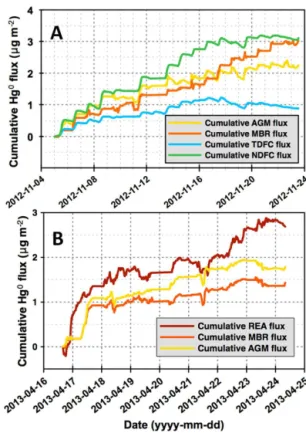
The cumulative flux derived by the examined methods is presented in Fig. 11a, b. During IC#1, the cumulative fluxes measured by MBR and AGM fell between the fluxes mea-sured by the two DFC methods. A period of divergence in the magnitude between the derived turbulent exchange parame-ters (eddy diffusivity of heat andυtr)resulted in intersected courses of MBR and AGM cumulative flux (17 November). MBR flux then stayed beyond the AGM flux on a cumula-tive basis for the rest of the campaign. The cumulacumula-tive flux gauged by the TDFC method was the lowest (approximately 1/3 of MBR flux). Over the duration of IC#1, the net Hg0 flux estimated by MBR and NDFC methods was in good agreement (2.90 vs. 3.02 µg m2)while the AGM method
de-Figure 11.Time series cumulative Hg0 flux using various tech-niques for(a)IC#1 over bare soil and(b)IC#2 over wheat canopy.
rived a∼25 % lower Hg0net evasion. This indicates that the
flux correction with synchronized surface shear properties in NDFC partially bridges frequently observed disparities in magnitude between the MM- and conventional chamber-derived fluxes (e.g., Gustin et al., 1999). Figure 12a shows the scatterplot of hourly flux specifically for MBR versus NDFC/TDFC – the correlation between individual hourly data points is weak. While in Fig. 12b, the deviation between MBR cumulative fluxes and NDFC/TDFC cumulative fluxes during the sampling campaign suggests that NDFC measure-ment shows a great advantage in bridging the flux gap be-tween DFCs and MBR measurement. The significant scat-tering in Fig. 12a stems substantially from the inherent high variability in MBR flux prevalent during daytime. The dif-ference between chamber and MBR flux depends to a certain degree on the diurnal variation of the atmospheric conditions. During daytime, the chamber produces a delay in the daytime flux evolution and fluxes become sustained in the late after-noon due to an artificial reduction in surface cooling within the chamber (Fig. 10).
During IC#2, the gradient-based MM techniques were evaluated together with the REA technique. The temporal features of the convoluted MBR and AGM cumulative fluxes are by and large concordant albeit the latter technique gauged
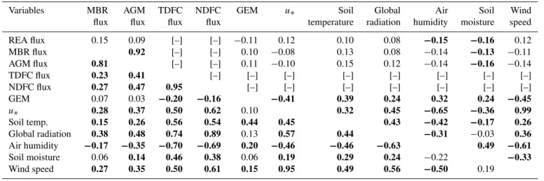
method-Table 2.Pearson correlation analysis of hourly Hg0flux from various field measurement techniques and environmental parameters for two campaigns. Top-right segment of data are from IC#2. Bold font denotes a statistically significant correlation coefficient (p <0.05).
Variables MBR AGM TDFC NDFC GEM u∗ Soil Global Air Soil Wind
flux flux flux flux temperature radiation humidity moisture speed
REA flux 0.15 0.09 [–] [–] −0.11 0.12 0.10 0.08 −0.15 −0.16 0.12
MBR flux 0.92 [–] [–] 0.10 −0.08 0.13 0.08 −0.14 −0.13 −0.11
AGM flux 0.81 [–] [–] 0.11 −0.10 0.15 0.12 −0.14 −0.16 −0.14
TDFC flux 0.23 0.41 [–] [–] [–] [–] [–] [–] [–] [–]
NDFC flux 0.27 0.47 0.95 [–] [–] [–] [–] [–] [–] [–]
GEM 0.07 0.03 −0.20 −0.16 −0.41 0.39 0.24 0.32 0.24 −0.45
u∗ 0.28 0.37 0.50 0.62 0.10 0.32 0.45 −0.65 −0.36 0.99
Soil temp. 0.15 0.26 0.56 0.54 0.44 0.45 0.43 −0.42 −0.17 0.26
Global radiation 0.38 0.48 0.74 0.89 0.13 0.57 0.44 −0.31 −0.03 0.36
Air humidity −0.17 −0.35 −0.70 −0.69 0.20 −0.46 −0.46 −0.63 0.49 −0.61
Soil moisture 0.06 0.14 0.46 0.38 0.06 0.19 0.29 0.24 −0.22 −0.33
Wind speed 0.27 0.35 0.50 0.61 0.15 0.95 0.49 0.56 −0.50 0.19
Figure 12.Scatterplots of(a)MBR vs. NDFC/TDFC Hg0flux and (b) time series cumulative flux difference between the MBR and NDFC/TDFC method.
ological limitations given by the diverging micrometeorolog-ical conditions (Zhu et al., 2015b). For an extended period, the cumulative flux of REA given in Fig. 11b evolved in a similar way to those of the gradient-based methods (18–21
April). However, considerably different fluxes, occasionally in reverse directions, occurred after 21 April. In particular, during 16–17 April (Fig. 11b), a large net emission event was observed by all three techniques but at different magnitude.
3.5 Correlation between Hg0flux observation and environmental factors
It has been shown that the air–surface exchange of Hg can be influenced by solar irradiation, temperature, humidity, mois-ture, wind shear condition, and biotic processes (Choi and Holsen, 2009; Eckley et al., 2010; Fu et al., 2008; Gustin, 2011; Zhu et al., 2013a; Lin et al., 2010), as also observed in our field (Figs. 9 and 10). Table 2 shows the Pearson correla-tion coefficients between Hg0fluxes measured by the differ-ent methods and meteorological variables. DFC Hg0 fluxes were positively correlated with solar radiation, soil tempera-ture, soil moistempera-ture, friction velocity (R∼0.4–0.9,p<0.05),
and negatively correlated with air Hg0 concentration and air humidity (p<0.05). The correlations between the MM fluxes and environmental variables were generally weaker (|R|<0.5) in both campaigns. It is evident that DFC is less sensitive to surrounding atmospheric conditions that control the MM flux. In contrast, the Hg0flux controls in the ecosys-tem enclosed by the chamber are subject to microenviron-ment conditions that are significantly perturbed foremost by solar heating.
4 Conclusions and implications
DFC-derived Hg0 fluxes showed distinct temporal charac-teristics. The former exhibited a highly dynamic variabil-ity while the latter had gradual temporal features. Diurnal trends showed that MM and DFC measurements diagnosed a similar daytime emission peak with different peaking times. Such differences were driven by separate sets of environ-mental factors influencing the DFC (irradiance and temper-ature) and MM (atmospheric turbulence properties) mea-surements. The three MM methods (REA, AGM and MBR) observed statistically significant, inseparable median Hg0 fluxes (p<0.05) albeit REA flux was distributed over a much broader scale. Gradient and DFCs methods inter-compared favorably with respect to the confined location of median fluxes. Instantaneous fluxes measured by NDFC and TDFC and by MBR and AGM methods respectively were highly correlated (R>0.8,p<0.05) as the pairwise techniques are based on the same theoretical concept. However, the compa-rability between individual DFC and MM fluxes was poor to moderate (R∼0.1–0.5) indicating the risk of utilizing spo-radic (non-diurnally resolved) flux measurements as repre-sentative of an ecosystem.
The five techniques gauged unanimously positive net Hg0 fluxes cumulated over the campaign periods. For the inves-tigated triad of MM techniques, the Hg0-REA system has a general tendency to derive fluxes largest in magnitude. Over most of the campaign time, REA reported 20–60 % higher cumulative flux compared to the AGM method next to REA. Intriguingly, the Hg0flux budget magnitude exam-ined by AGM and MBR methods was reversed during the two campaigns with a difference of∼20 %, which may
re-sult from the atmospheric conditions and proxy scalar be-havior. The traditional DFC method systematically measured the lowest Hg0 net emission (42 % and 31 % of AGM- and MBR-derived net emission, respectively). The NDFC tech-nique measured averaged fluxes similar to turbulent Hg0 fluxes obtained by the MBR method (5.3 % difference). Al-though not entirely coupled to the atmospheric conditions that control the flux, the NDFC technique nevertheless rep-resents a significant progress and improvement in contempo-rary enclosure-based Hg0flux measurement.
It was feasible to obtain a gradient measurement height ratio at the recommended bound (Foken, 2008). Given the lower precision of REA, gradient-based methods are conse-quently recommended for atmosphere–ecosystem Hg0 flux measurements over low vegetation. REA has its niche over tall canopy, where gradient methods have frequently been found impracticable. In future applications, concerning fore-most MM flux measurement technique, where the capacity to resolve small concentration differences is critical, it is rec-ommended to implement analysis of synchronously collected samples for various heights (AGM, MBR) and conditionally segregated air parcels (REA) to avoid uncertainties induced by non-uniform ambient air Hg0 concentration during the flux-averaging period. It has recently been argued that direct measurement of Hg0ecosystem air-canopy gas exchange is
difficult and potentially subject to larger uncertainties (Zhang et al., 2012). Nevertheless, it is practicable for Hg0as it is for other trace gases and aerosols for which continuous MM flux measurement systems are key tools in ecosystem sciences. Our results show that improvement in resolving small Hg0 concentration differences for the MM systems is required to further reduce uncertainties in the flux estimation.
Acknowledgements. This research was financially supported by
“973 Program” (2013CB430002), National Science Foundation of China (41030752), Chinese Academy of Sciences through an instrument development program (YZ200910), and the State Key Laboratory of Environmental Geochemistry. We would thank the staff from Yucheng Comprehensive Experimental Station, Chinese Academy of Sciences for their sampling assistance.
Edited by: L. Zhang
References
Aubinet, M., Vesala, T., and Papale, D.: Eddy Covariance: a Prac-tical Guide to Measurement and Data Analysis, Springer, Dor-drecht, the Netherlands, 2012.
Bahlmann, E., Ebinghaus, R., and Ruck, W.: Development and application of a laboratory flux measurement system (LFMS) for the investigation of the kinetics of mercury emissions from soils, J. Environ. Manage., 81, 114–125, doi:10.1016/j.jenvman.2005.09.022, 2006.
Bash, J. O.: Description and initial simulation of a dynamic bidi-rectional air-surface exchange model for mercury in Commu-nity Multiscale Air Quality (CMAQ) model, J. Geophys. Res.-Atmos., 115, D06305, doi:10.1029/2009JD012834, 2010. Bash, J. O. and Miller, D. R.: A relaxed eddy accumulation system
for measuring surface fluxes of total gaseous mercury, J. Atmos. Ocean. Tech., 25, 244–257, doi:10.1175/2007JTECHA908.1, 2008.
Bash, J. O. and Miller, D. R.: Growing season total gaseous mercury (TGM) flux measurements over anAcer rubrumL. stand, Atmos.
Environ., 43, 5953–5961, doi:10.1016/j.atmosenv.2009.08.008, 2009.
Baya, A. P. and Van Heyst, B.: Assessing the trends and effects of environmental parameters on the behaviour of mercury in the lower atmosphere over cropped land over four seasons, At-mos. Chem. Phys., 10, 8617–8628, doi:10.5194/acp-10-8617-2010, 2010.
Beverland, I. J., Oneill, D. H., Scott, S. L., and Moncrieff, J. B.: Design, construction and operation of flux measurement systems using the conditional sampling technique, Atmos. Environ., 30, 3209–3220, doi:10.1016/1352-2310(96)00010-6, 1996. Carpi, A. and Lindberg, S. E.: Application of a Teflon (TM)
dy-namic flux chamber for quantifying soil mercury flux: tests and results over background soil, Atmos. Environ., 32, 873–882, doi:10.1016/S1352-2310(97)00133-7, 1998.
temper-ature and UV radiation, Environ. Pollut., 157, 1673–1678, doi:10.1016/j.envpol.2008.12.014, 2009.
Cobbett, F. D. and Van Heyst, B. J.: Measurements of GEM fluxes and atmospheric mercury concentrations (GEM, RGM and Hg-P) from an agricultural field amended with biosolids in Southern Ont., Canada (October 2004-November 2004), Atmos. Environ., 41, 2270–2282, doi:10.1016/j.atmosenv.2006.11.011, 2007. Cobos, D. R. and Baker, J. M.: Conditional sampling for
mea-suring mercury vapor fluxes, Atmos. Environ., 36, 4309–4321, doi:10.1016/S1352-2310(02)00400-4, 2002.
Converse, A. D., Riscassi, A. L., and Scanlon, T. M.: Sea-sonal variability in gaseous mercury fluxes measured in a high-elevation meadow, Atmos. Environ., 44, 2176–2185, doi:10.1016/j.atmosenv.2010.03.024, 2010.
Durnford, D., Dastoor, A., Figueras-Nieto, D., and Ryjkov, A.: Long range transport of mercury to the Arctic and across Canada, Atmos. Chem. Phys., 10, 6063–6086, doi:10.5194/acp-10-6063-2010, 2010.
Eckley, C. S., Gustin, M., Lin, C. J., Li, X., and Miller, M. B.: The influence of dynamic chamber design and operating parameters on calculated surface-to-air mercury fluxes, Atmos. Environ., 44, 194–203, doi:10.1016/j.atmosenv.2009.10.013, 2010.
Edwards, G. C., Rasmussen, P. E., Schroeder, W. H., Kemp, R. J., Dias, G. M., Fitzgerald-Hubble, C. R., Wong, E. K., Halfpenny-Mitchell, L., and Gustin, M. S.: Sources of variability in mercury flux measurements, J. Geophys. Res.-Atmos., 106, 5421–5435, doi:10.1029/2000JD900496, 2001.
Edwards, G. C., Rasmussen, P. E., Schroeder, W. H., Wal-lace, D. M., Halfpenny-Mitchell, L., Dias, G. M., Kemp, R. J., and Ausma, S.: Development and evaluation of a sampling sys-tem to determine gaseous Mercury fluxes using an aerodynamic micrometeorological gradient method, J. Geophys. Res.-Atmos., 110, D10306, doi:10.1029/2004jd005187, 2005.
Farmer, D. K., Wooldridge, P. J., and Cohen, R. C.: Application of thermal-dissociation laser induced fluorescence (TD-LIF) to measurement of HNO3, 6alkyl nitrates,6peroxy nitrates, and NO2 fluxes using eddy covariance, Atmos. Chem. Phys., 6, 3471–3486, doi:10.5194/acp-6-3471-2006, 2006.
Feng, X. B., Wang, S. F., Qiu, G. L., Hou, Y. M., and Tang, S. L.: Total gaseous mercury emissions from soil in Guiyang, Guizhou, China, J. Geophys. Res.-Atmos., 110, D14306, doi:10.1029/2004JD005643, 2005.
Foken, T.: Micrometeorology, Springer-Verlag, Berlin, Heidelberg, 306 pp., 2008.
Fowler, D., Hargreaves, K. J., Skiba, U., Milne, R., Zahniser, M. S., Moncrieff, J. B., Beverland, I. J., and Gallagher, M. W.: Mea-surements of CH4and N2O fluxes at the landscape scale using micrometeorological methods, Phil. Trans. Phys. Sci. Eng., 351, 339–355, 1995.
Fritsche, J., Obrist, D., Zeeman, M. J., Conen, F., Eugster, W., and Alewell, C.: Elemental mercury fluxes over a sub-alpine grass-land determined with two micrometeorological methods, Atmos. Environ., 42, 2922–2933, doi:10.1016/j.atmosenv.2007.12.055, 2008a.
Fritsche, J., Wohlfahrt, G., Ammann, C., Zeeman, M., Ham-merle, A., Obrist, D., and Alewell, C.: Summertime elemen-tal mercury exchange of temperate grasslands on an ecosystem-scale, Atmos. Chem. Phys., 8, 7709–7722, doi:10.5194/acp-8-7709-2008, 2008b.
Fu, X., Feng, X., Zhang, H., Yu, B., and Chen, L.: Mercury emis-sions from natural surfaces highly impacted by human activities in Guangzhou province, South China, Atmos. Environ., 54, 185– 193, doi:10.1016/j.atmosenv.2012.02.008, 2012.
Fu, X. W., Feng, X. B., and Wang, S. F.: Exchange fluxes of Hg between surfaces and atmosphere in the eastern flank of Mount Gongga, Sichuan province, southwestern China, J. Geophys. Res.-Atmos., 113, D20306, doi:10.1029/2008JD009814, 2008. Fu, X. W., Feng, X. B., Wan, Q., Meng, B., Yan, H. Y., and
Guo, Y. N.: Probing Hg evasion from surface waters of two Chi-nese hyper/meso-eutrophic reservoirs, Sci. Total Environ., 408, 5887–5896, doi:10.1016/j.scitotenv.2010.08.001, 2010. Gustin, M. and Jaffe, D.: Reducing the Uncertainty in Measurement
and Understanding of Mercury in the Atmosphere, Environ. Sci. Technol., 44, 2222–2227, doi: 10.1021/es902736k, 2010. Gustin, M. S.: Exchange of mercury between the atmosphere and
terrestrial ecosystems, in: Environmental Chemisty and Toxicol-ogy of Mercury, edited by: Liu, G. L., Cai, Y., and O’Driscoll, N., doi:10.1002/9781118146644, 423–451, 2011.
Gustin, M. S. and Lindberg, S. E.: Assessing the contribution of nat-ural sources to the global mercury cycle: the importance of inter-comparing dynamic flux measurements, Fresen. J. Anal. Chem., 366, 417–422, doi:10.1007/s002160050085, 2000.
Gustin, M. S., Lindberg, S., Marsik, F., Casimir, A., Ebing-haus, R., Edwards, G., Hubble-Fitzgerald, C., Kemp, R., Kock, H., Leonard, T., London, J., Majewski, M., Monteci-nos, C., Owens, J., Pilote, M., Poissant, L., Rasmussen, P., Schaedlich, F., Schneeberger, D., Schroeder, W., Sommar, J., Turner, R., Vette, A., Wallschlaeger, D., Xiao, Z., and Zhang, H.: Nevada STORMS project: measurement of mercury emissions from naturally enriched surfaces, J. Geophys. Res.-Atmos., 104, 21831–21844, doi:10.1029/1999JD900351, 1999.
Hensen, A., Nemitz, E., Flynn, M. J., Blatter, A., Jones, S. K., Sørensen, L. L., Hensen, B., Pryor, S. C., Jensen, B., Otjes, R. P., Cobussen, J., Loubet, B., Erisman, J. W., Gallagher, M. W., Nef-tel, A., and Sutton, M. A.: Inter-comparison of ammonia fluxes obtained using the Relaxed Eddy Accumulation technique, Bio-geosciences, 6, 2575–2588, doi:10.5194/bg-6-2575-2009, 2009. Hou, R., Ouyang, Z., Li, Y., Tyler, D. D., Li, F., and Wilson, G. V.: Effects of tillage and residue management on soil organic carbon and total nitrogen in the North China Plain, Soil Sci. Soc. Am. J., 76, 230–240, doi:10.2136/sssaj2011.0107, 2012.
Kaimal, J., Wyngaard, J., Izumi, Y., and Coté, O.: Spectral charac-teristics of surface-layer turbulence, Q. J. Roy. Meteor. Soc., 98, 563–589, doi:10.1002/qj.49709841707, 1972.
Kim, K. H., Kim, M. Y., Kim, J., and Lee, G.: Effects of changes in environmental conditions on atmospheric mercury exchange: comparative analysis from a rice paddy field during the two spring periods of 2001 and 2002, J. Geophys. Res.-Atmos., 108, 4607, doi:10.1029/2003JD003375, 2003.
Kljun, N., Calanca, P., Rotach, M., and Schmid, H.: A simple parameterisation for flux footprint pre-dictions, Bound.-Lay. Meteorol., 112, 503–523, doi:10.1023/B:BOUN.0000030653.71031.96, 2004.
Kormann, R. and Meixner, F. X.: An analytical footprint model for non-neutral stratification, Bound.-Lay. Meteorol., 99, 207–224, doi:10.1023/A:1018991015119, 2001.
air-borne mercury from five municipal solid waste landfills in Guiyang and Wuhan, China, Atmos. Chem. Phys., 10, 3353– 3364, doi:10.5194/acp-10-3353-2010, 2010.
Lin, C.-J., Gustin, M. S., Singhasuk, P., Eckley, C., and Miller, M.: Empirical models for estimating mercury flux from soils, En-viron. Sci. Technol., 44, 8522–8528, doi:10.1021/es1021735, 2010.
Lin, C.-J., Zhu, W., Li, X., Feng, X., Sommar, J., and Shang, L.: Novel dynamic flux chamber for measuring air–surface ex-change of Hg0 from soils, Environ. Sci. Technol., 46, 8910– 8920, doi:10.1021/es3012386, 2012.
Lindberg, S. E., Kim, K. H., Meyers, T. P., and Owens, J. G.: Mi-crometeorological gradient approach for quantifying air-surface exchange of mercury vapor: tests over contaminated soils, En-viron. Sci. Technol., 29, 126–135, doi:10.1021/es00001a016, 1995.
Lindqvist, O., Johansson, K., Bringmark, L., Timm, B., Aastrup, M., Andersson, A., Hovsenius, G., Håkanson, L., Iverfeldt, Å., and Meili, M.: Mercury in the Swedish environment – Recent research on causes, consequences and corrective methods, Water Air Soil Pollut., 55, xi-261, doi:10.1007/BF00542429, 1991. Liu, H. and Foken, T.: A modified Bowen ratio method to determine
sensible and latent heat fluxes, Meteorologische Zeitschrift, 10, 71–80, doi:10.1127/0941-2948/2001/0010-0071, 2001. Marsik, F. J., Keeler, G. J., Lindberg, S. E., and Zhang, H.:
Air-surface exchange of gaseous mercury over a mixed sawgrass-cattail stand within the Florida Everglades, Environ. Sci. Tech-nol., 39, 4739–4746, doi:10.1021/es0404015, 2005.
Mauder, M. and Foken, T.: Documentation and instruction man-ual of the eddy covariance software package TK2, Vol. 26, Arbeitsergebnisse, Universitat Bayreuth, Abteilung Mikromete-orologie. Universitat Bayreuth, Abteilung Mikrometeorologie, Bayreuth, 42 pp., ISSN 1614–8916, 2004.
Mauder, M., Cuntz, M., Drüe, C., Graf, A., Rebmann, C., Schmid, H. P., Schmidt, M., and Steinbrecher, R.: A strat-egy for quality and uncertainty assessment of long-term eddy-covariance measurements, Agr. Forest Meteorol., 169, 122–135, doi:10.1016/j.agrformet.2012.09.006, 2013.
Moncrieff, J. B., Beverland, I. J., ÓNéill, D. H., and Crop-ley, F. D.: Controls on trace gas exchange observed by a con-ditional sampling method, Atmos. Environ., 32, 3265–3274, doi:10.1016/S1352-2310(97)00506-2, 1998.
Monin, A. and Obukhov, A.: Basic laws of turbulent mixing in the surface layer of the atmosphere, Acad. Nauk. SSR. Trud. Geofiz. Inst., 151, 163–187, 1954.
National Atmospheric Deposition Program (NADP): Atmospheric Mercury Network Operations Manual (2011–05) Version 1.0., http://nadp.isws.illinois.edu/amn/docs/AMNet_Operations_ Manual.pdf, NADP Program Office, 2204 Griffith Dr., Cham-paign, IL 61820, 2011.
Nemitz, E., Flynn, M., Williams, P., Milford, C., Theobald, M., Blatter, A., Gallagher, M., and Sutton, M.: A relaxed eddy accumulation system for the automated measurement of at-mospheric ammonia fluxes, Water Air Soil Poll., 1, 189–202, doi:10.1023/A:1013103122226, 2001.
Nemitz, E., Loubet, B., Lehmann, B. E., Cellier, P., Neftel, A., Jones, S. K., Hensen, A., Ihly, B., Tarakanov, S. V., and Sut-ton, M. A.: Turbulence characteristics in grassland canopies and
implications for tracer transport, Biogeosciences, 6, 1519–1537, doi:10.5194/bg-6-1519-2009, 2009.
Olofsson, M., Sommar, J., Ljungström, E., and Andersson, M.: Ap-plication of relaxed eddy accumulation techniques to qualify Hg0 fluxes over modified soil surfaces, Water Air Soil Poll., 167, 331– 354, doi:10.1007/s11270-005-0012-8, 2005.
Panofsky, H. A. and Dutton, J. A.: Atmospheric Turbulence, Models and Methods for Engineering Applications, John Wiley & Sons, New York, 1984.
Park, J.-H., Goldstein, A., Timkovsky, J., Fares, S., Weber, R., Karlik, J., and Holzinger, R.: Active atmosphere-ecosystem ex-change of the vast majority of detected volatile organic com-pounds, Science, 341, 643–647, doi:10.1126/science.1235053, 2013.
Pirrone, N., Cinnirella, S., Feng, X., Finkelman, R. B., Friedli, H. R., Leaner, J., Mason, R., Mukherjee, A. B., Stra-cher, G. B., Streets, D. G., and Telmer, K.: Global mercury emis-sions to the atmosphere from anthropogenic and natural sources, Atmos. Chem. Phys., 10, 5951–5964, doi:10.5194/acp-10-5951-2010, 2010.
Poissant, L. and Casimir, A.: Water-air and soil-air exchange rate of total gaseous mercury measured at background sites, Atmos. Environ., 32, 883–893, doi:10.1016/S1352-2310(97)00132-5, 1998.
Poissant, L., Pilote, M., and Casimir, A.: Mercury flux measure-ments in a naturally enriched area: correlation with environmen-tal conditions during the Nevada Study and Tests of the Release of Mercury From Soils (STORMS), J. Geophys. Res.-Atmos., 104, 21845–21857, doi:10.1029/1999JD900092, 1999.
Poissant, L., Pilote, M., Xu, X. H., Zhang, H., and Beauvais, C.: Atmospheric mercury speciation and deposition in the Bay St. Francois wetlands, J. Geophys. Res.-Atmos., 109, D11301, doi:10.1029/2003jd004364, 2004.
Simpson, I., Edwards, G., Thurtell, G., Den Hartog, G., Neu-mann, H., and Staebler, R.: Micrometeorological measure-ments of methane and nitrous oxide exchange above a bo-real aspen forest, J. Geophys. Res.-Atmos., 102, 29331–29341, doi:10.1029/97JD03181, 1997.
Sommar, J., Zhu, W., Lin, C.-J., and Feng, X.: Field ap-proaches to measure Hg exchange between natural sur-faces and the atmosphere – a review, Critical Reviews in Environmental Science and Technology, 43, 1657–1739, doi:10.1080/10643389.2012.671733, 2013a.
Sommar, J., Zhu, W., Shang, L., Feng, X., and Lin, C.-J.: A whole-air relaxed eddy accumulation measurement system for sampling vertical vapour exchange of elemental mercury, Tellus B, 65, 19940, doi:10.3402/tellusb.v65i0.19940, 2013b.
Stamenkovic, J. and Gustin, M. S.: Evaluation of use of Eco-CELL technology for quantifying total gaseous mercury fluxes over background substrates, Atmos. Environ., 41, 3702–3712, doi:10.1016/j.atmosenv.2006.12.037, 2007.
Twine, T. E., Kustas, W., Norman, J., Cook, D., Houser, P., Mey-ers, T., Prueger, J., Starks, P., and Wesely, M.: Correcting eddy-covariance flux underestimates over a grassland, Agr. Forest Meteorol., 103, 279–300, doi:10.1016/S0168-1923(00)00123-4, 2000.
modi-fied Bowen-ratio technique, Agr. Forest Meteorol., 138, 54–68, doi:10.1016/j.agrformet.2006.03.011, 2006.
Wallschlager, D., Turner, R. R., London, J., Ebinghaus, R., Kock, H. H., Sommar, J., and Xiao, Z. F.: Factors affect-ing the measurement of mercury emissions from soils with flux chambers, J. Geophys. Res.-Atmos., 104, 21859–21871, doi:10.1029/1999JD900314, 1999.
Wang, S. F., Feng, X. B., Qiu, G. L., Wei, Z. Q., and Xiao, T. F.: Mercury emission to atmosphere from Lanmuchang Hg-Tl min-ing area, Southwestern Guizhou, China, Atmos. Environ., 39, 7459–7473, doi:10.1016/j.atmosenv.2005.06.062, 2005. Wang, S. F., Feng, X. B., Qiu, G. L., Fu, X. W., and Wei, Z. Q.:
Characteristics of mercury exchange flux between soil and air in the heavily air-polluted area, eastern Guizhou, China, Atmos. Environ., 41, 5584–5594, doi:10.1016/j.atmosenv.2007.03.002, 2007.
Wesely, M. L. and Hicks, B. B.: A review of the current status of knowledge on dry deposition, Atmos. Environ., 34, 2261–2282, doi:10.1016/S1352-2310(99)00467-7, 2000.
Whitehead, J. D., Twigg, M., Famulari, D., Nemitz, E., Sut-ton, M. A., Gallagher, M. W., and Fowler, D.: Evaluation of laser absorption spectroscopic techniques for eddy covariance flux measurements of ammonia, Environ. Sci. Technol., 42, 2041– 2046, doi:10.1021/es071596u, 2008.
Xiao, Z. F., Munthe, J., Schroeder, W. H., and Lindqvist, O.: Vertical fluxes of volatile mercury over forest soil and lake surfaces in Sweden, Tellus B, 43, 267–279, doi:10.3402/tellusb.v43i3.15274, 1991.
Zhang, H., Lindberg, S. E., Barnett, M. O., Vette, A. F., and Gustin, M. S.: Dynamic flux chamber measurement of gaseous mercury emission fluxes over soils, Part 1: Simulation of gaseous mercury emissions from soils using a two-resistance exchange interface model, Atmos. Environ., 36, 835–846, doi:10.1016/S1352-2310(01)00501-5, 2002.
Zhang, L. M., Wright, L. P., and Blanchard, P.: A review of current knowledge concerning dry deposition of at-mospheric mercury, Atmos. Environ., 43, 5853–5864, doi:10.1016/j.atmosenv.2009.08.019, 2009.
Zhang, L., Blanchard, P., Gay, D. A., Prestbo, E. M., Risch, M. R., Johnson, D., Narayan, J., Zsolway, R., Holsen, T. M., Miller, E. K., Castro, M. S., Graydon, J. A., Louis, V. L. S., and Dalziel, J.: Estimation of speciated and total mercury dry deposition at monitoring locations in eastern and central North America, At-mos. Chem. Phys., 12, 4327–4340, doi:10.5194/acp-12-4327-2012, 2012.
Zhang, L., Wang, S. X., Wang, L., and Hao, J. M.: Atmospheric mercury concentration and chemical speciation at a rural site in Beijing, China: implications of mercury emission sources, Atmos. Chem. Phys., 13, 10505–10516, doi:10.5194/acp-13-10505-2013, 2013.
Zhu, W., Li, Z., Chai, X., Hao, Y., Lin, C.-J., Sommar, J., and Feng, X.: Emission characteristics and air–surface exchange of gaseous mercury at the largest active landfill in Asia, Atmos. Environ., 79, 188–197, doi:10.1016/j.atmosenv.2013.05.083, 2013a.
Zhu, W., Sommar, J., Li, Z., Feng, X., Lin, C.-J., and Li, G.: Highly elevated emission of mercury vapor due to the spontaneous com-bustion of refuse in a landfill, Atmos. Environ., 79, 540–545, doi:10.1016/j.atmosenv.2013.07.016, 2013b.
Zhu, W., Sommar, J., Lin, C.-J., Feng, X. B., Shang, L. H., and Zhang, Y. T.: Seasonal elemental mercury gas exchange over a wheat-corn rotation cropland in the North China Plain, unpub-lished data, 2015a.