Top-down constraints on atmospheric mercury emissions and implications for global biogeochemical cycling

(1)

ACPD

15, 5269–5325, 2015

Top-down constraints on atmospheric mercury emissions

S. Song et al.

Title Page

Abstract Introduction

Conclusions References

Tables Figures

◭ ◮

Back Close

Full Screen / Esc

Printer-friendly Version Interactive Discussion

Discussion

P

a

per

|

Discussion

P

a

per

|

Discussion

P

a

per

|

Discussion

P

a

per

|

Atmos. Chem. Phys. Discuss., 15, 5269–5325, 2015 www.atmos-chem-phys-discuss.net/15/5269/2015/ doi:10.5194/acpd-15-5269-2015

This discussion paper is/has been under review for the journal Atmospheric Chemistry and Physics (ACP). Please refer to the corresponding final paper in ACP if available.

Top-down constraints on atmospheric

mercury emissions and implications for

global biogeochemical cycling

S. Song1, N. E. Selin1,2, A. L. Soerensen3,4, H. Angot5, R. Artz6, S. Brooks7,

E.-G. Brunke8, G. Conley9, A. Dommergue5, R. Ebinghaus10, T. M. Holsen11,

D. A. Jaffe12,13, S. Kang14,15, P. Kelley6,16, W. T. Luke6, O. Magand5, K. Marumoto17, K. A. Pfaffhuber18, X. Ren6,16, G.-R. Sheu19, F. Slemr20,

T. Warneke21, A. Weigelt10, P. Weiss-Penzias22, D. C. Wip23, and Q. Zhang24

1

Department of Earth, Atmospheric and Planetary Sciences, Massachusetts Institute of Technology, Cambridge, MA, USA

2

Engineering Systems Division, Massachusetts Institute of Technology, Cambridge, MA, USA

3

Department of Environmental Health, Harvard School of Public Health, Boston, MA, USA

4

Department of Applied Environmental Science, Stockholm University, Stockholm, Sweden

5

Univ. Grenoble Alpes, CNRS, LGGE, Grenoble, France

6

Air Resources Laboratory, National Oceanic and Atmospheric Administration, College Park, MD, USA

7

(2)

ACPD

15, 5269–5325, 2015

S. Song et al.

Title Page

Tables Figures

◭ ◮

Back Close

Full Screen / Esc

Discussion

P

a

per

|

Discussion

P

a

per

|

Discussion

P

a

per

|

Discussion

P

a

per

|

8

South African Weather Service c/o CSIR, Stellenbosch, South Africa

9

Center for Air Quality, Ohio University, Athens, OH, USA

10

Institute of Coastal Research, Helmholtz-Zentrum Geesthacht, Geesthacht, Germany

11

Department of Civil and Environmental Engineering, Clarkson University, Potsdam, NY, USA

12

School of Science, Technology, Engineering and Mathematics, University of Washington, Bothell, WA, USA

13

Department of Atmospheric Sciences, University of Washington, Seattle, WA, USA

14

State Key Laboratory of Cryospheric Sciences, Cold and Arid Regions Environmental and Engineering Research Institute, Chinese Academy of Sciences (CAS), Lanzhou, China

15

CAS Center for Excellence in Tibetan Plateau Earth Sciences, Chinese Academy of Sciences, Beijing, China

16

Cooperative Institute for Climate and Satellites, University of Maryland, College Park, MD, USA

17

Environmental Chemistry Section, National Institute for Minamata Disease, Kumamoto, Japan

18

Norwegian Institute for Air Research (NILU), Norway

19

Department of Atmospheric Sciences, National Central University, Jhongli, Taiwan

20

Max Planck Institute for Chemistry, Air Chemistry Division, Mainz, Germany

21

Institute of Environmental Physics, University of Bremen, Germany

22

Microbiology and Environmental Toxicology, University of California, Santa Cruz, CA, USA

23

Anton de Kom Universiteit van Suriname, Paramaribo, Suriname

24

Key Laboratory of Tibetan Environment Changes and Land Surface Processes, Institute of Tibetan Plateau Research, Chinese Academy of Sciences, Beijing, China

Received: 26 November 2014 – Accepted: 7 February 2015 – Published: 25 February 2015 Correspondence to: S. Song (song33@mit.edu)

Published by Copernicus Publications on behalf of the European Geosciences Union.

(3)

ACPD

15, 5269–5325, 2015

S. Song et al.

Title Page

Tables Figures

◭ ◮

Back Close

Full Screen / Esc

Discussion

P

a

per

|

Discussion

P

a

per

|

Discussion

P

a

per

|

Discussion

P

a

per

|

Abstract

We perform global-scale inverse modeling to constrain present-day atmospheric mer-cury emissions and relevant physio-chemical parameters in the GEOS-Chem chemi-cal transport model. We use Bayesian inversion methods combining simulations with GEOS-Chem and ground-based Hg0observations from regional monitoring networks

5

and individual sites in recent years. Using optimized emissions/parameters, GEOS-Chem better reproduces these ground-based observations, and also matches regional over-water Hg0and wet deposition measurements. The optimized global mercury emis-sion to the atmosphere is ∼5.8 Gg yr−1. The ocean accounts for 3.2 Gg yr−1 (55 % of the total), and the terrestrial ecosystem is neither a net source nor a net sink of Hg0.

10

The optimized Asian anthropogenic emission of Hg0(gas elemental mercury) is 650– 1770 Mg yr−1, higher than its bottom-up estimates (550–800 Mg yr−1). The ocean pa-rameter inversions suggest that dark oxidation of aqueous elemental mercury is faster, and less mercury is removed from the mixed layer through particle sinking, when com-pared with current simulations. Parameter changes affect the simulated global ocean

15

mercury budget, particularly mass exchange between the mixed layer and subsurface waters. Based on our inversion results, we re-evaluate the long-term global biogeo-chemical cycle of mercury, and show that legacy mercury becomes more likely to reside in the terrestrial ecosystem than in the ocean. We estimate that primary anthropogenic mercury contributes up to 23 % of present-day atmospheric deposition.

20

1 Introduction

Mercury (Hg) is a ubiquitous trace metal that cycles among the atmosphere, ocean, land, and biosphere (Selin, 2009). Atmospheric mercury transports globally (Driscoll et al., 2013), and in aquatic systems, can be converted to methylmercury, a bioaccu-mulative toxic compound (Mergler et al., 2007). Human activities have strongly affected

25

(4)

ACPD

15, 5269–5325, 2015

S. Song et al.

Title Page

Tables Figures

◭ ◮

Back Close

Full Screen / Esc

Discussion

P

a

per

|

Discussion

P

a

per

|

Discussion

P

a

per

|

Discussion

P

a

per

|

2011). Since mercury deposited to terrestrial and ocean surfaces can remobilize, the atmosphere continues to be a_ffected by its historical releases (Lindberg et al., 2007; Amos et al., 2013). Atmosphere–surface fluxes of mercury are still poorly constrained, limiting our ability to fully understand timescales of its global biogeochemical cycle (Pir-rone et al., 2010; Mason et al., 2012). A better knowledge of these fluxes is important

5

for assessing its human impacts and evaluating effectiveness of policy actions (Selin, 2014).

Current estimates of mercury fluxes to the atmosphere are mainly built on a bottom-up approach. Anthropogenic inventories are based on emission factors, activity lev-els, and abatement efficiency (Pacyna et al., 2010; Wang, S. et al., 2014; Muntean

10

et al., 2014). Flux estimates from ocean and terrestrial surfaces extrapolate limited di-rect measurements to larger scales and use simplified process models (Mason, 2009; Kuss et al., 2011). The top-down or inverse approach, combining observations and at-mospheric modeling, has been widely used to derive sources and sinks of greenhouse gases and ozone-depleting substances (Gurney et al., 2002; Xiao et al., 2010).

In-15

verse studies have addressed mercury at regional scale (Roustan and Bocquet, 2006; Krüger et al., 1999). For example, a hybrid inversion combining back trajectories and a regional chemical transport model (CTM) identified Hg0emission using year-long ur-ban observations (de Foy et al., 2012). This scheme was expanded to estimate sources of oxidized Hg (de Foy et al., 2014).

20

In this paper, we apply a top-down approach at global scale to quantitatively estimate present-day mercury emission sources (emission inversion) as well as key parameters in a CTM (parameter inversion), in order to better constrain the global biogeochemical cycle of mercury. Section 2 describes the overall methodology. We combine ground-based observations of atmospheric Hg0 (Sect. 2.1) and simulations with the

GEOS-25

Chem global CTM (Sect. 2.2). Reference (also known as a priori) emissions are from GEOS-Chem parameterizations and agree well with bottom-up estimates (Sect. 2.3). We adopt a Bayesian inversion method (Sect. 2.4) to obtain the optimized (a posteri-ori) emissions, with a monthly time step, taking into account uncertainties associated

(5)

ACPD

15, 5269–5325, 2015

S. Song et al.

Title Page

Tables Figures

◭ ◮

Back Close

Full Screen / Esc

Discussion

P

a

per

|

Discussion

P

a

per

|

Discussion

P

a

per

|

Discussion

P

a

per

|

with both reference emissions and ground-based observations (Sect. 2.6). Section 3 presents results and discussion. Comparisons of observations and model outputs are given in Sect. 3.1. The optimized emissions from ocean and terrestrial surfaces and from anthropogenic sources are shown in Sect. 3.2. We use results of the emission inversion to identify key uncertain model parameters, and optimize them in the

param-5

eter inversion (Sects. 2.5 and 3.3). Finally, we discuss implications of our inversion results for the global biogeochemical mercury cycle (Sect. 3.4) and summarize our conclusions (Sect. 4).

2 Methods

2.1 Atmospheric mercury observations

10

Tropospheric mercury exists mainly as gaseous elemental mercury (GEM) but also as two operationally defined species, gaseous oxidized mercury (GOM) and particle-bound mercury (PBM) (Valente et al., 2007). Manual methods of measuring GEM or total gaseous mercury (TGM=GEM+GOM) were applied in the 1970s (Slemr et al., 1981). High-frequency measurements (time resolution <1 h, e.g. using Tekran

auto-15

mated ambient air analyzers) became available in the 1990s and have substantially replaced manual sampling (time resolution of about several hours). We only use GEM and TGM observations in this study because we are not able to quantify the uncertainty in GOM and PBM measurements (Ja_ffe et al., 2014; McClure et al., 2014).

We identify high-frequency observations of GEM and TGM concentration for our

in-20

versions using two criteria. First, we choose sites in rural/remote areas not strongly a_ffected by local emission. Second, we require that observations at di_fferent sites are minimally correlated (Brunner et al., 2012). Data sets are drawn from the Atmospheric Mercury Network (AMNet) (Gay et al., 2013), the Canadian Measurement Networks (including the Canadian Air and Precipitation Monitoring Network (CAPMoN) and other

25

(6)

Mon-ACPD

15, 5269–5325, 2015

S. Song et al.

Title Page

Tables Figures

◭ ◮

Back Close

Full Screen / Esc

Discussion

P

a

per

|

Discussion

P

a

per

|

Discussion

P

a

per

|

Discussion

P

a

per

|

itoring and Evaluation Programme (EMEP) (Tørseth et al., 2012). We use data from 2009–2011, when all these networks were active. To expand spatial coverage of ob-servations, we also collected data from individual sites for recent years (2007–2013). Some sites are included in the Global Mercury Observation System (GMOS) (Pirrone et al., 2013). All sites use Tekran analyzers, operated in sampling intervals of 5–30 min.

5

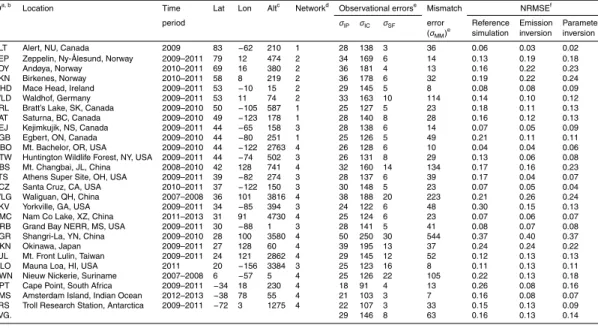
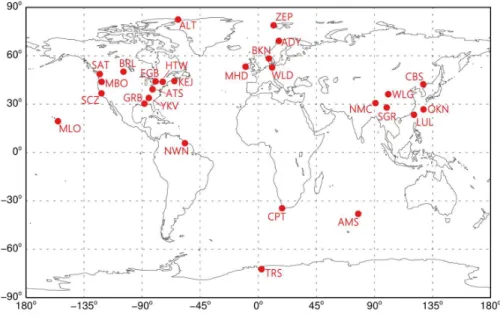
We calculate the Pearson’s correlation coefficients between each two pair of sites us-ing hourly data. Several sites are excluded due to strong correlations within each other, as shown in the Supplement, Table S1. Table 1 shows the names, locations, and a_ffi l-iated networks of the 27 ground-based sites used in our inversion. Site locations are also plotted in Fig. 1. For most of these sites GEM data are used, and for a few sites

10

where GEM data are not available we use TGM data (see Table 1). The concentra-tion difference in remote near-surface air is usually <1 % (Lan et al., 2012; Fu et al., 2012a; Weigelt et al., 2013; Steffen et al., 2014), and thus we do not distinguish be-tween measured GEM and TGM concentrations and use Hg0 to represent them in the paper. These sites are all uncorrelated or only weakly correlated (₋0.3< r <0.4,

15

n=103−104) (see Table S2 in the Supplement).

Original observational data are converted into hourly averages and then into monthly averages (Fig. S1 in the Supplement). We require >30 min data to derive an hourly average and>10 day data to derive a monthly average. Where full data are available, median values are used to suppress the influence of high Hg0 due to local or regional

20

pollution events (Weigelt et al., 2013; Ja_ffe et al., 2005) or occasional low Hg0 due to non-polar depletion events (Brunke et al., 2010). For a few individual sites (see Table 1), the original data are not available, and monthly arithmetic means are used. Finally, multiple-year averages are calculated. Hg0concentrations are given in ng m−3

at standard temperature and pressure.

25

Four polar sites are included (ALT, ZEP, and ADY in Arctic and TRS in Antarctica, see Table 1). Episodically low Hg0is observed at these sites in polar spring (Cole et al., 2013; Pfaffhuber et al., 2012). These atmospheric mercury depletion events (AMDEs) result from rapid Hg0oxidation and deposition driven by halogens (Steffen et al., 2008).

(7)

ACPD

15, 5269–5325, 2015

S. Song et al.

Title Page

Tables Figures

◭ ◮

Back Close

Full Screen / Esc

Discussion

P

a

per

|

Discussion

P

a

per

|

Discussion

P

a

per

|

Discussion

P

a

per

|

Volatilization of deposited Hg and river input may contribute to the observed summer Hg0peak (Dastoor and Durnford, 2013; Fisher et al., 2012). The lack of understanding of above physical and chemical processes limits GEOS-Chem’s ability to reproduce Hg0 in the polar spring and summer. For these reasons we remove Hg0 data at polar sites for this period (i.e. March–September in Arctic and October–March in Antarctica).

5

We also include three mountain-top sites (LUL, MBO, and MLO, see Table 1). These sites are affected by upslope surface air during the day and downslope air from the free troposphere at night (Sheu et al., 2010; Fu et al., 2010). The downslope air usually contains higher levels of GOM than the upslope air does due to oxidation of Hg0 to GOM in the free troposphere (Timonen et al., 2013). Therefore, Hg0 at mountain-top

10

sites peaks in the afternoon whereas GOM peaks between midnight and early morning (Fig. S2 in the Supplement), showing an opposite diurnal pattern to most low-elevation sites (Lan et al., 2012). The minimum hourly Hg0 at night is calculated to be ∼90 % of the all-day average. Thus, to represent Hg0 modeled at a vertical layer in the free troposphere (this layer is obtained by matching observed air pressure), the observed

15

mountain-top Hg0data are multiplied by 0.9.

We do not use over-water Hg0observations (i.e. from ship cruises) in the inversion because they are very limited and usually cover large areas, making their observational errors difficult to estimate. Instead, we use over-water observations as an independent check of our inversion results. The North Atlantic Ocean is the most densely

sam-20

pled ocean basin. Soerensen et al. (2012) assembled Hg0measurements from 18 ship cruises in this region during 1990–2009 and found a statistically significant decrease of−0.046±0.010 ng m−3yr−1. However, previous GEOS-Chem simulations of Hg0 con-centration did not take this multi-decadal trend into account in evaluating its seasonal variability (Soerensen et al., 2010a). Here we add a new ship cruise and adjust

ob-25

(8)

ACPD

15, 5269–5325, 2015

S. Song et al.

Title Page

Tables Figures

◭ ◮

Back Close

Full Screen / Esc

Discussion

P

a

per

|

Discussion

P

a

per

|

Discussion

P

a

per

|

Discussion

P

a

per

|

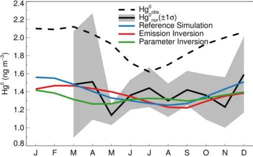
measurement. As shown in Fig. 2, Hg0_nor are smaller and show less seasonal variability compared to Hg0_obs.

2.2 GEOS-Chem model

GEOS-Chem (v9-02) is a CTM driven by assimilated meteorological fields from the NASA Goddard Earth Observing System (GEOS) (Bey et al., 2001). The original

5

GEOS-5 has a resolution of 1/2◦

×2/3◦ and is degraded to 2◦×2.5◦ for input into our simulations. The GEOS-Chem global mercury simulation was described and eval-uated in Selin et al. (2007) and Strode et al. (2007), with updates by Selin et al. (2008), Holmes et al. (2010), Soerensen et al. (2010b), and Amos et al. (2012). It couples a three-dimensional atmosphere, a dimensional mixed layer slab ocean, and a

two-10

dimensional terrestrial reservoir. For consistency with most ground-based observa-tions, we use meteorological years of 2009–2011 for analysis, after a spin-up period of four years.

Three mercury tracers (representing GEM, GOM, and PBM) are simulated in the atmosphere in GEOS-Chem. Models have assumed that Hg0is oxidized by OH, ozone,

15

and/or halogens (Lei et al., 2013; De Simone et al., 2014; Travnikov and Ilyin, 2009; Durnford et al., 2010; Grant et al., 2014). Some studies suggested that gas-phase reaction with Br was the most important Hg0oxidation process globally (Seigneur and Lohman, 2008; Hynes et al., 2009), and here we use Br as the only oxidant of Hg0 (Holmes et al., 2010; Goodsite et al., 2012). Tropospheric Br fields are archived from

20

a full chemistry GEOS-Chem simulation (Parrella et al., 2012). Models also hypothesize gas- and/or aqueous-phase reductions of oxidized Hg and scale their kinetics to match atmospheric observations (Holmes et al., 2010; Pongprueksa et al., 2011; Selin et al., 2007). However, an accurate determination of potential pathways is lacking (Subir et al., 2011, 2012), and their atmospheric relevance is unknown (Gårdfeldt and Jonsson,

25

2003). Thus we do not include atmospheric reduction of oxidized Hg in our simulations.

(9)

ACPD

15, 5269–5325, 2015

S. Song et al.

Title Page

Tables Figures

◭ ◮

Back Close

Full Screen / Esc

Discussion

P

a

per

|

Discussion

P

a

per

|

Discussion

P

a

per

|

Discussion

P

a

per

|

2.3 Emission inversion: reference emissions

For our reference emissions, we use parameterizations in GEOS-Chem with improve-ments from recent literature. As shown in Table 2, global mercury emission is estimated as 6.0 Gg yr−1_{, with an uncertainty range of 0.4–12.2 Gg yr}−1_{. Mercury released via} nat-ural processes is assumed to be entirely Hg0(Stein et al., 1996), while a small fraction

5

of anthropogenic mercury is in oxidized forms. Anthropogenic emission is unidirec-tional, but air–surface exchange is bi-directional (emission and deposition) (Xu et al., 1999; Gustin et al., 2008). A positive net emission from a surface means it is a net source of Hg0, whereas a negative value means it is a net sink. We describe below our reference emissions for individual sources.

10

2.3.1 Anthropogenic sources

We use the anthropogenic emission inventory based on activity data for year 2010, developed by AMAP/UNEP (2013). As shown in Table 2, the total anthropogenic emis-sion is 1960 Mg yr−1_{, with an uncertainty range of 1010–4070 Mg yr}−1 _(AMAP/UNEP, 2013). We do not optimize oxidized mercury emissions (accounting for 19 % of the

to-15

tal anthropogenic sources) because this form has a short atmospheric lifetime (days to weeks) and may not significantly contribute to observed Hg0. The geospatial distri-bution for emissions from contaminated sites (Kocman et al., 2013) is not available for this inventory, and we distribute this small source (80 Mg yr−1) based on the locations of mercury mines (Selin et al., 2007). We do not consider in-plume reduction of oxidized

20

Hg emitted from coal-fired power plants (Zhang, Y. et al., 2012). About 50 % of global emissions are from Asia (defined as 65–146◦E, 9◦S–60◦N), and a small fraction are from Europe and North America (together <10 %). For other regions like Africa and South America, there is no e_ffective observational site to constrain emissions (Fig. 1). Thus, only anthropogenic emissions from Asia are optimized in the inversion, but we

25

(10)

ACPD

15, 5269–5325, 2015

S. Song et al.

Title Page

Tables Figures

◭ ◮

Back Close

Full Screen / Esc

Discussion

P

a

per

|

Discussion

P

a

per

|

Discussion

P

a

per

|

Discussion

P

a

per

|

2.3.2 Ocean

The mixed layer (ML) slab ocean model in GEOS-Chem is described in Soerensen et al. (2010b). Net Hg0 emission from ocean surfaces is determined by the supersat-uration of Hg0_aq in the ML relative to the atmosphere and the air–sea exchange rate. Hg0_aq in the ML is mainly produced by the net photolytic and biotic reduction of Hg2_aq+.

5

Atmospheric deposition accounts for most Hg2_aq+ inputs into the ML, but subsurface wa-ters also contribute a considerable fraction. The ML interacts with subsurface wawa-ters through entrainment/detrainment of the ML and wind-driven Ekman pumping.

We improve several parameterizations in GEOS-Chem based on recent findings. (1) Basin-specific subsurface water mercury concentrations are updated according to new

10

measurements (Lamborg et al., 2012; Munson, 2014), as shown in the Supplement, Fig. S4. (2) Soerensen et al. (2010b) used the Wilke–Chang method for estimating the Hg0_aqdiffusion coefficient (D_Hg) (Wilke and Chang, 1955), but this estimate was believed to be too high (Loux, 2004). We adopt a revisedD_Hg derived by molecular dynamics (MD) simulation (Kuss et al., 2009). As shown in the Supplement, Fig. S5, compared

15

to the Wilke–Chang method, MD simulation obtains a D_Hg that agrees much better with laboratory results (Kuss, 2014). (3) Particulate mercury (HgP_aq) sinking from the ML is estimated by linking the organic carbon export (biological pump) and HgP_aq: C ratios. Soerensen et al. (2010b) used the model of Antia et al. (2001) for estimating carbon export fluxes, giving a global total of 23 Gt C yr−1_{. However, this estimate is}

20

mainly based on the flux measurement data from much deeper depths and may not well represent carbon export from the ML. Di_fferent models suggest global carbon export fluxes ranging from 5–20 Gt C yr−1 _{with a best estimate of 11 Gt C yr}−1 _{(Sanders et al.,}

2014; Henson et al., 2011). Thus, we multiply carbon export fluxes in GEOS-Chem by a factor of 0.47 (11 Gt C yr−1_/_{23 Gt C yr}−1_{) to match this best estimate.}

25

Net global ocean emission of 2990 Mg yr−1_{from the improved GEOS-Chem}

(consid-ered as reference emission, shown in Table 2) compares favorably with best estimates of 2680 Mg yr−1_{using a bottom-up approach (Pirrone et al., 2010; Mason, 2009). Due to}

(11)

ACPD

15, 5269–5325, 2015

S. Song et al.

Title Page

Tables Figures

◭ ◮

Back Close

Full Screen / Esc

Discussion

P

a

per

|

Discussion

P

a

per

|

Discussion

P

a

per

|

Discussion

P

a

per

|

their different seasonal characteristics, we divide the global ocean into the NH (North-ern Hemisphere) and SH (South(North-ern Hemisphere) oceans, and optimize their emissions separately.

2.3.3 Terrestrial ecosystem

Although atmosphere–terrestrial Hg0 exchange is bi-directional, only recently

devel-5

oped exchange models have coupled deposition (downward) and emission (upward) fluxes and dynamically estimated net fluxes by gradients between air Hg0 and “com-pensation points” inferred from surface characteristics (Bash, 2010; Bash et al., 2007). Because their complex parameterizations lack field data for verification (Wang, X. et al., 2014), such exchange models have not been incorporated into current global CTMs.

10

As described in Selin et al. (2008) and Holmes et al. (2010), GEOS-Chem treats emis-sion and deposition fluxes of Hg0separately. Only dry deposition is considered for Hg0 due to its low Henry’s law constant (Lin and Pehkonen, 1999). Net emission from ter-restrial surfaces (E_net) represents the sum of these processes: volatilization from soil (E_soil), prompt reemission of deposited Hg (E_pr), geogenic activity (E_gg), biomass

burn-15

ing (E_bb), and dry deposition to surfaces (E_ddHg0).

E_net=E_soil+E_pr+E_gg+E_bb−EddHg0 (1)

Soil emission (Esoil) is specified as a function of solar radiation and soil Hg

concen-tration:

E_soil(ng m−2_h−1₎

=βC_soilexp(1.1×10−3×Rg) (2)

20

where C_soil is soil Hg concentration (ng g−1_{) and} _R

g is the solar radiation flux

(12)

ACPD

15, 5269–5325, 2015

S. Song et al.

Title Page

Tables Figures

◭ ◮

Back Close

Full Screen / Esc

Discussion

P

a

per

|

Discussion

P

a

per

|

Discussion

P

a

per

|

Discussion

P

a

per

|

10−2_{g m}−2_h−1_{) is obtained from the global mass balance of the preindustrial}

simula-tion. Selin et al. (2008) assumed that present-day soil mercury reservoir and emission have both increased by 15 % compared to preindustrial period, and distributed this global average increase according to the present-day deposition pattern of anthro-pogenic emission. However, by linking soil mercury with organic carbon pools,

Smith-5

Downey et al. (2010) estimated that present-day Hg storage in organic soils has in-creased by 20 % while soil emission by 190 %. Mason and Sheu (2002) suggested doubled soil emissions compared to preindustrial times. Thus, following Smith-Downey et al. (2010), we assume a 190 % global increase in the present-day, and distribute this increase according to the anthropogenic emission deposition pattern. The present-day

10

reference soil emission is calculated to be 1680 Mg yr−1.

An additional 520 Mg yr−1_{is emitted from the soil, vegetation, and snow (}_E

pr) through

rapid photoreduction of recently deposited oxidized Hg (Fisher et al., 2012). Geogenic emission (E_gg) is set as 90 Mg yr−1, consistent with its best bottom-up estimate (Ma-son, 2009; Bagnato et al., 2014). Biomass burning (E_bb) of 210 Mg yr−1 is estimated

15

using the Global Fire Emissions Database version 3 of CO (van der Werf et al., 2010) and a Hg : CO ratio of 100 nmol mol−1 _{(Holmes et al., 2010). This amount falls at the} lower end of bottom-up estimates (Friedli et al., 2009). Dry deposition of Hg0 is esti-mated using a resistance-in-series scheme (Wesely, 1989) and has a downward flux of 1430 Mg yr−1_{. Using Eq. (1), net emission of Hg}0_{from terrestrial surfaces is calculated}

20

to be 1070 Mg yr−1 _{in GEOS-Chem (Table 2), at the lower end of the bottom-up}

esti-mates (1140–5280 Mg yr−1) (Mason, 2009; Pirrone et al., 2010), and also lower than 1910 Mg yr−1 _{by Kikuchi et al. (2013) using a di}

fferent empirical mechanism (Lin et al., 2010).

2.3.4 Sources included in emission inversion

25

Because of limitations in both observations and the CTM, only anthropogenic emission from Asia, ocean evasion (separated into the NH and SH), and soil emission are

(13)

ACPD

15, 5269–5325, 2015

S. Song et al.

Title Page

Tables Figures

◭ ◮

Back Close

Full Screen / Esc

Discussion

P

a

per

|

Discussion

P

a

per

|

Discussion

P

a

per

|

Discussion

P

a

per

|

mized in the emission inversion (see Table 2). The remaining sources are still included in the simulation but not inverted because they are too di_ffusely distributed, their mag-nitude is small, and/or observations are not sensitive to them (Chen and Prinn, 2006). The seasonal sources (the NH ocean, SH ocean, and soil) usually have strong spa-tiotemporal variations and the inversion optimizes their monthly magnitudes and

uncer-5

tainties. For the aseasonal Asian anthropogenic emission, the inversion optimizes its annual magnitude and uncertainty.

2.4 Bayesian inversion method

We use a Bayesian method to invert emissions and parameters with a weighted least-squares technique (Ulrych et al., 2001). Unknowns (correction factors for reference

10

emissions and parameters) are contained in a state vectorx and their a priori errors (uncertainties in reference emissions and parameters) in a matrixP. It assumes a linear relationship between the observation vectoryobsandx, as shown in the measurement equation:

yobs=yref+Hx+ǫ (3)

15

where the vectoryref contains monthly Hg0 concentrations modeled by GEOS-Chem using reference emissions and parameters, andǫrepresents model and observational errors.xis related to concentrations by the sensitivity matrixH, in which the elements are written as:

H_{i j} =(y_i−yref_i )/(x_j₋xref_j )_≈∂y_i/∂x_j (4)

20

wherei andjare indices for the observation and state vector, respectively.Hdescribes how monthly Hg0concentrations at each observational site respond to changes in the state vector (for examples see the Supplement, Fig. S6). The objective functionJwith respect toxis:

J(x)₌xTP−1x+(Hx−yobs+yref)TR−1(Hx−yobs+yref) (5)

(14)

ACPD

15, 5269–5325, 2015

S. Song et al.

Title Page

Tables Figures

◭ ◮

Back Close

Full Screen / Esc

Discussion

P

a

per

|

Discussion

P

a

per

|

Discussion

P

a

per

|

Discussion

P

a

per

|

where the matrixRrepresents errors related to observations and the CTM and is de-scribed in detail in Sect. 2.6. By minimizing J, we obtain expression for the optimal estimate ofx:

x=(HTR−1H+P−1)−1HTR−1(yobs₋yref) (6)

Q=(HTR−1_H₊_P−1₎−1 ₍₇₎

5

where the matrixQcontains the a posteriori errors ofx. A detailed mathematical deriva-tion of the above equaderiva-tions can be found in Wunsch (2006).

2.5 Parameter inversion

As described below in Sect. 3.2.1, based on results of ocean evasion in our emission inversion and sensitivity tests of model parameters, we identify two ocean parameters

10

in GEOS-Chem for improvement: the rate constant of dark oxidation of Hg0_aq (denoted as K_OX2, following notations in Soerensen et al., 2010b)) and the partition coe_fficient between Hg2_aq+ and HgP_aq (denoted asKD). For simplicity they are expressed in

logarith-mic forms (₋logK_OX2 and logK_D).

A−logKOX2(s−1) of 7.0 is specified in GEOS-Chem (Soerensen et al., 2010b). From

15

a survey of laboratory studies (see details in the Supplement) (Amyot et al., 1997; Lalonde et al., 2001, 2004; Qureshi et al., 2010), we suggest that this value is too low and that a more appropriate range of−logKOX2 is 4.0–6.0. The chemical mechanisms

for dark oxidation of Hg0_aq remain unclear. OH generated from photochemically pro-duced H₂O₂via the Fenton reaction may oxidize Hg0_aq in dark conditions (Zhang and

20

Lindberg, 2001; Zepp et al., 1992). Light irradiation before a dark period is needed, and dark oxidation kinetics depend on intensity and duration of light (Qureshi et al., 2010; Batrakova et al., 2014). Future work could include a more mechanistic representation of this process as laboratory studies become available.

K_D(=C_s/C_dC_SPM) describes the affinity of aqueous Hg2+ for suspended particulate

25

(15)

ACPD

15, 5269–5325, 2015

S. Song et al.

Title Page

Tables Figures

◭ ◮

Back Close

Full Screen / Esc

Discussion

P

a

per

|

Discussion

P

a

per

|

Discussion

P

a

per

|

Discussion

P

a

per

|

SPM, respectively. GEOS-Chem uses a logK_D(L kg−1_{) of 5.5 based on measurements}

in North Pacific and North Atlantic Ocean (Mason and Fitzgerald, 1993; Mason et al., 1998).

In the parameter inversion, we attempt to constrain these two ocean model parame-ters using the Bayesian approach described in Sect. 2.4. For consistency with sources

5

in the emission inversion, two other parameters are included, i.e. emission ratios for soil (ER_Soil) and Asian anthropogenic sources (ER_Asia). Because the responses of Hg0 concentrations to changes in ocean parameters are nonlinear, as shown in the Supple-ment, Fig. S7, we use a two-step iterative inversion method (Prinn et al., 2011). At each iteration step, the sensitivity matrixHis estimated by linearizing the nonlinear function

10

around the current parameter estimate.

2.6 Error representation

Successful estimation ofx (Eq. 6) and its uncertainty Q(Eq. 7) depends on reason-able representations of all relevant errors, including the a priori errors associated with reference emissions/parameters (contained in P) and errors related to Hg0

observa-15

tions and the CTM (contained in R). R consists of three parts: observational errors, model–observation mismatch errors, and model errors.

2.6.1 Errors in reference emission and parameters

For the emission inversion, we set the one-sigma errors in reference emissions as 50 % in order to match uncertainties in their estimates using bottom-up approaches

20

(see Table 2). For example, the reference emissions and one-sigma errors for the NH and SH oceans are 1230±630 and 1760±880 Mg yr−1, respectively. The uncertainty range of reference emission from the global ocean is estimated as 470–5510 Mg yr−1_, comparing very well with 780–5280 Mg yr−1 _{from bottom-up estimates (Mason, 2009;}

Pirrone et al., 2010). For the parameter inversion, the a priori estimates of two ocean

25

(16)

ACPD

15, 5269–5325, 2015

S. Song et al.

Title Page

Tables Figures

◭ ◮

Back Close

Full Screen / Esc

Discussion

P

a

per

|

Discussion

P

a

per

|

Discussion

P

a

per

|

Discussion

P

a

per

|

(5.0±1.0) and logKD (5.3±0.4). The a priori uncertainties of ERSoil and ERAsia are

chosen as 50 %, the same as in the emission inversion.

2.6.2 Observational errors

Observational errors for ground-based sites determine their relative importance in de-riving the optimized state. As shown in Eq. (8), the total observational errors (σTOT)

5

contain instrumental precision (σ_IP), intercomparison (σ_IC), and sampling frequency er-rors (σ_SF) (Rigby et al., 2012; Chen and Prinn, 2006).

σ_TOT=

q

σ_IP2 +σ_IC2 +σ_SF2 (8)

The instrumental precision (σ_IP) of high-frequency Hg0measurements using the Tekran instrument is∼2 % (Poissant et al., 2005). The comparability of the Tekran instruments

10

has been assessed during several field intercomparisons (Temme et al., 2006; Aspmo et al., 2005; Munthe et al., 2001; Ebinghaus et al., 1999; Schroeder et al., 1995). Hg0 concentrations measured by di_fferent laboratories have a relative SD of reproducibility of 1–9 %, and we choose a generous uniform intercomparison error (σ_IC) of 10 %. Sampling frequency error (σ_SF) reflects the ability of each site to capture the overall

15

variability of Hg0 concentration in one month, and is calculated as the monthly SD divided by the square root of the number of valid hourly data points in this month (Rigby et al., 2012). Table 1 shows observational errors at each site, averaged over 2009–2011. The total observational errors are dominated by intercomparison errors. The other two types of errors have small contributions.

20

2.6.3 Model–observation mismatch errors

The mismatch error (σ_MM) exists because an observation is made at a single point in space but its corresponding grid box in model represents a large volume of air. We estimateσ_MM as the SD of monthly Hg0 concentrations in the eight surrounding grid

(17)

ACPD

15, 5269–5325, 2015

S. Song et al.

Title Page

Tables Figures

◭ ◮

Back Close

Full Screen / Esc

Discussion

P

a

per

|

Discussion

P

a

per

|

Discussion

P

a

per

|

Discussion

P

a

per

|

boxes (at the same vertical layer) from the reference simulation (Chen and Prinn, 2006). As shown in Table 1,σ_MMare larger over strongly emitting continental areas (e.g. SGR and WLG) and smaller over remote marine areas (e.g. CPT and AMS).

2.6.4 Model errors

All existing CTMs including GEOS-Chem are imperfect, due to both errors in

meteoro-5

logical data driving the CTMs and errors induced by their parameterizations of physical and chemical processes. The former type of model errors is termed “forcing errors” and the latter “process errors” (Locatelli et al., 2013). Physical processes consist of hori-zontal/vertical resolution, advection/convection, turbulence, planetary boundary layer mixing, etc. The CTM for Hg is subject to large process errors due to highly uncertain

10

atmospheric chemistry. Recent studies have showed that Br concentration may be sig-nificantly underestimated in GEOS-Chem (Parrella et al., 2012; Gratz et al., 2015) and that current Br-initiated oxidation mechanisms are incomplete in describing all possible radical reactions (Dibble et al., 2012; Wang, F. et al., 2014). In order to provide a prelim-inary assessment of the e_ffect of Br oxidation chemistry on our inversion, we perform

15

an additional parameter inversion including six new elements in the state vectorx, and each of them represents Br columns in a 30◦latitudinal band (see results in Sect. 3.3 and Fig. S8 in the Supplement).

Quantifying model errors requires incorporating many CTMs which are driven by dif-ferent meteorology and which contain different parameterizations (Prinn, 2000).

Multi-20

CTM intercomparison studies have been performed for CO₂ and CH₄ (Gurney et al., 2002; Baker et al., 2006; Locatelli et al., 2013), suggesting that model errors can impact inverted emissions. Few other global CTMs exist for Hg (Bullock et al., 2008, 2009). Due to our inability to quantify model errors using a single CTM, model errors are not incorporated in our inversion, like many other inverse studies (Huang et al., 2008; Xiao

25

(18)

ACPD

15, 5269–5325, 2015

S. Song et al.

Title Page

Tables Figures

◭ ◮

Back Close

Full Screen / Esc

Discussion

P

a

per

|

Discussion

P

a

per

|

Discussion

P

a

per

|

Discussion

P

a

per

|

3 Results and discussion

3.1 Emission inversion: model–observation comparison

We first test whether the comparison between ground-based Hg0 observations and model outputs improves when using optimized emissions, compared to reference emis-sions. Figure 3 shows the modeled and observed Hg0 concentrations at all 27 sites.

5

To quantify model performance, we calculate the normalized root mean square error (NRMSE) for each site:

NRMSE=

v u u t 1

n

X

i=1

(X_obs,_i−Xmod,i)2

1

n

X

i=1

X_obs,_i (9)

whereXobs,i and Xmod,i are the observed and modeled Hg0 concentrations at the ith

month (n in total), respectively. As shown in Table 1, an average NRMSE of 0.13 is

10

obtained for the emission inversion, smaller than that of 0.16 for the reference simula-tion, indicating that the emission inversion can better reproduce ground-based obser-vations. While this is a relatively small uncertainty reduction (₋0.03), we do not expect better performance for our inversion. This is because errors in Hg0 observations (as described above, and in Table 1) are roughly 13 %, which constrain the optimization.

15

Our inversion brings the average NRMSE within the observation error.

The NRMSEs are not reduced for all 27 sites (see Table 1). For three Nordic sites (ZEP, ADY, and BKN) and four Asia-Pacific sites (WLG, SGR, LUL, and MLO), the NRMSEs increase. Hg0 concentrations are _∼1.8 ng m−3 _{at the three Nordic sites,} higher than the modeled values (Fig. 3) from both reference simulation and emission

20

inversion, and also higher than those measured at many background sites in Europe (Ebinghaus et al., 2011; Kentisbeer et al., 2014; Weigelt et al., 2013). Part of the dif-ferences may be explained by a positive bias in the instrumentation of these Nordic observations when compared to other laboratories (Temme et al., 2006). It is also pos-sible that GEOS-Chem cannot su_fficiently capture local meteorology and/or emissions

25

(19)

ACPD

15, 5269–5325, 2015

S. Song et al.

Title Page

Tables Figures

◭ ◮

Back Close

Full Screen / Esc

Discussion

P

a

per

|

Discussion

P

a

per

|

Discussion

P

a

per

|

Discussion

P

a

per

|

at these sites. For the Asia-Pacific sites, the reference simulation underestimates Hg0 at SGR (−32 %, calculated as (yref/yobs₋1)_×100 %, hereinafter the same) and WLG (−19 %), and predicts comparable values at MLO (+2 %) and LUL (+0 %). Such dis-crepancies likely arise from unknown intercomparison errors and influence by local emission and meteorology factors not captured by the CTM (Fu et al., 2012b; Wan

5

et al., 2009). These sites are operated by three different laboratories, but to the best of our knowledge, no field intercomparisons have been conducted among these labora-tories.

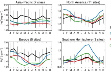
Figure 4 compares monthly Hg0 observations with model simulations for sites ag-gregated into four regions: Asia-Pacific, North America, Europe, and Southern

Hemi-10

sphere (SH). The emission inversion significantly improves the comparison for the SH sites (CPT, AMS, and TRS, see Table 1). In the reference simulation, Hg0 concentra-tions at the SH sites vary seasonally, with a high in austral winter (∼1.3 ng m−3) and a low in austral summer (_∼0.9 ng m−3_{). However, observed Hg}0 _{shows little seasonal}

variation with monthly concentrations of∼ 1.0 ng m−3. The emission inversion reduces

15

Hg0 concentration in austral winter and fits the observations much better (the average NRMSE decreases from 0.19 to 0.10). As shown in Fig. 3, all three SH sites show improvement after optimization.

The emission inversion also improves the comparison for sites in North America (the average NRMSE decreases from 0.13 to 0.08). Hg0 data at a total of 11 sites are

20

available, including five coastal sites (ALT, SAT, KEJ, SCZ, and GRB), five inland sites (BRL, EGB, HTW, ATS, and YKV), and one mountain-top site (MBO) (see Fig. 1 and Table 1). Hg0at the coastal and inland sites are observed to be 1.41_±0.04 and 1.29_± 0.06 ng m−3, respectively. This coastal–inland difference in observation is consistent with results of Cheng et al. (2014), who found that air masses from open ocean at

25

the site KEJ had 0.06 ng m−3 _{higher Hg}0 _{concentrations than those originating over}

(20)

ACPD

15, 5269–5325, 2015

S. Song et al.

Title Page

Tables Figures

◭ ◮

Back Close

Full Screen / Esc

Discussion

P

a

per

|

Discussion

P

a

per

|

Discussion

P

a

per

|

Discussion

P

a

per

|

sites, the emission inversion predicts Hg0concentrations (1.38_±0.03 ng m−3_{) closer to}

observations than the reference simulation (1.50±0.06 ng m−3).

Over-water Hg0observations serve as an independent test of the emission inversion. As shown in Fig. 2, Hg0concentrations over the North Atlantic Ocean from both the ref-erence simulation and the emission inversion fall within one-sigma uncertainty ranges

5

of Hg0_nor. The NRMSEs for the reference simulation and the emission inversion are 0.09 and 0.10, respectively. Thus using Hg0 emissions constrained by ground-based observations, GEOS-Chem still matches these regional over-water observations.

We additionally test performance of the inversion by comparison with regional wet deposition data. Since most oxidized Hg is formed from the oxidation of Hg0, changing

10

Hg0emissions may have an effect on modeled oxidized Hg and its subsequent deposi-tion. We compare model results to the observed wet deposition fluxes from NADP/MDN (2012), as shown in the Supplement, Fig. S9. We use the monitoring sites active in 2009–2011 (n=126). Both the reference simulation and the emission inversion fit ob-servations well (R≈0.7, NRMSE≈0.3). Accordingly, the effect of the inversion on the

15

NADP/MDN wet deposition fluxes is insignificant.

3.2 Emission inversion: optimized emissions

The annual reference and optimized emissions of mercury are shown in Table 2. The

relationship ¯σ=

s

nPn

i=1

σ_t2, where n=12 months and σ_t is monthly error, is used to compute the annual uncertainty for seasonal processes (Chen and Prinn, 2006). The

20

uncertainty of the aseasonal source (annual Asian anthropogenic emission) is ob-tained directly from Eq. (7). The global optimized mercury emission is _∼5.8 Gg yr−1_,

with an uncertainty range of 1.7–10.3 Gg yr−1. Compared to our reference emission of ∼6.0 Gg yr−1 (uncertainty range: 0.4–12.2 Gg yr−1), the emission inversion results in a slightly smaller value and also reduces its uncertainty range. The optimized value is

25

smaller than previous estimates of 7.5 Gg yr−1by Pirrone et al. (2010) using a

(21)

ACPD

15, 5269–5325, 2015

S. Song et al.

Title Page

Tables Figures

◭ ◮

Back Close

Full Screen / Esc

Discussion

P

a

per

|

Discussion

P

a

per

|

Discussion

P

a

per

|

Discussion

P

a

per

|

up approach. The emission inversion increases emissions from anthropogenic sources and ocean surfaces, but decreases those from terrestrial surfaces. The ocean ac-counts for more than half (55 %) of the total, while the terrestrial surface contributes only a small fraction (6 %).

3.2.1 Ocean

5

Net Hg0 evasion from the global ocean is optimized by the emission inversion as 3160 Mg yr−1, with an uncertainty range of 1160–5160 Mg yr−1 (Table 2). The NH and SH oceans contribute similar amounts to the total, but on an area basis, evasion from the NH ocean is higher since it is 30 % smaller. We are able to reduce ocean evasion uncertainty from 50 to 40 % by using top-down constraints.

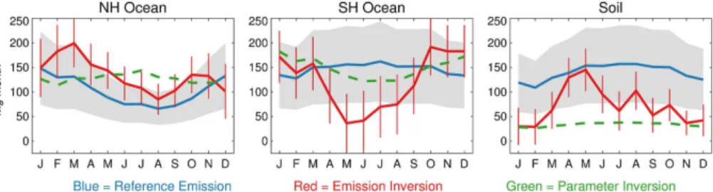
10

Figure 5 shows the monthly reference and optimized emissions of seasonal sources. We find, for both hemispheres, that the emission inversion generally results in in-creased ocean emissions in summer and dein-creased emissions in winter, compared to the reference simulation. As a result, we hypothesize that one or more ocean pro-cesses that a_ffect the seasonal behavior of aqueous mercury and its evasion are not

15

well-represented in GEOS-Chem. We therefore conduct a series of sensitivity studies of model parameters to test their potential effects on the seasonal pattern of ocean emission. We also compare the parameter values used in GEOS-Chem with their pos-sible ranges in a recent review (Batrakova et al., 2014). The tested model parameters in GEOS-Chem include rates of redox chemical reactions and physical processes in

20

the ML and subsurface mercury concentrations a_ffecting physical exchange between the ML and subsurface waters. Through these sensitivity tests and literature review, we identify two processes as candidates for improvement, the rate constant of dark oxidation of Hg_aq0 (K_OX2) and the partition coe_fficient between Hg_aq2+ and HgP_aq (K_D). We optimize these two ocean model parameters in the parameter inversion, as described

25

(22)

ACPD

15, 5269–5325, 2015

S. Song et al.

Title Page

Tables Figures

◭ ◮

Back Close

Full Screen / Esc

Discussion

P

a

per

|

Discussion

P

a

per

|

Discussion

P

a

per

|

Discussion

P

a

per

|

3.2.2 Terrestrial ecosystem

As shown in Table 2, the emission inversion reduces soil emissions of Hg0 by about 50 %, from 1680±840 to 860±440 Mg yr−1. Using Eq. (1), the optimized net emis-sion flux from terrestrial surfaces (Enet) is 340 Mg yr−1. If we do not consider

ge-ogenic activities (90 Mg yr−1_{) and biomass burning (210 Mg yr}−1_{), the}_E

net2 (calculated

5

asE_soil+E_pr−EddHg0 and representing net emissions from soils/vegetation) is almost

zero after optimization. Thus terrestrial surfaces are neither a net source nor a net sink of Hg0. This is in contrast to bottom-up estimates that the terrestrial surface is a net source of about 2000 Mg yr−1(Pirrone et al., 2010; Mason, 2009).

Vegetation is now believed to serve as a net sink of atmospheric Hg0 through foliar

10

uptake and sequestration (Gustin et al., 2008; Stamenkovic and Gustin, 2009; Wang, X. et al., 2014). Although its size has not been well quantified, we suggest that this sink is important in global mass balance since litterfall transfers 2400–6000 Mg Hg yr−1 _to terrestrial surfaces (Gustin et al., 2008). Air-soil flux measurements show that Hg0 emissions from background soils generally dominate over dry deposition (Obrist et al.,

15

2014; Edwards and Howard, 2013; Park et al., 2013; Denkenberger et al., 2012; Er-icksen et al., 2006). Our result of a smaller soil Hg source is consistent with a study by Obrist et al. (2014), which suggested that Hg was unlikely to be re-emitted once incorporated into soils and that terrestrial Hg emission was restricted to surface layers (Demers et al., 2013). Our result is also in agreement with estimates of terrestrial fluxes

20

of southern Africa using Hg0correlations with222Rn, a radioactive gas of predominantly terrestrial origin (Slemr et al., 2013). Considering that soil is a smaller source while veg-etation a sink of Hg0, our result that the terrestrial ecosystem is neither a net source nor a net sink of Hg0is reasonable, implying that the magnitudes of soil emission and dry deposition of Hg0 (primarily to vegetation) are similar. We evaluate dry deposition

25

fluxes modeled by GEOS-Chem against data in Zhang, L. et al. (2012), which estimated fluxes at sites in North America and obtained good agreements with surrogate surface and litterfall measurements (Graydon et al., 2008; Lyman et al., 2007). As shown in

(23)

ACPD

15, 5269–5325, 2015

S. Song et al.

Title Page

Tables Figures

◭ ◮

Back Close

Full Screen / Esc

Discussion

P

a

per

|

Discussion

P

a

per

|

Discussion

P

a

per

|

Discussion

P

a

per

|

the Supplement, Fig. S10, there is no bias in the average dry deposition flux at eight background sites, indicating that _∼1400 Mg yr−1 _{(modeled by GEOS-Chem) may be} reasonable estimates for both emission and dry deposition of Hg0.

3.2.3 Anthropogenic emission from Asia

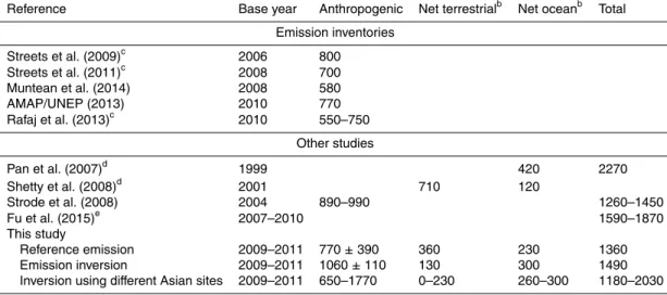
Table 3 summarizes Asian emissions of Hg0 (only GEM) estimated by several

re-5

cent bottom-up emission inventories and modeling studies. These inventories reported Asian anthropogenic emissions ranging from 550–800 Mg yr−1_{. In our model}

simula-tions, the reference emission of 770 Mg yr−1follows AMAP/UNEP (2013). The emission inversion using all 27 sites increases this value to 1060±110 Mg yr−1. Uncertainty in Asian anthropogenic emission should be larger than that obtained using our inversion

10

method, because emission estimates are sensitive to the Asia-Pacific sites used in the inversion. As discussed above, model performance at several Asia-Pacific sites is a_ffected by unknown intercomparison errors and local emission and meteorological fac-tors not captured by GEOS-Chem. To obtain a more accurate estimate of uncertainty, we perform seven emission inversions, each including only one Asia-Pacific site.

15

As shown in Table 3, these inversions result in Asian anthropogenic emissions of Hg0 ranging from 650–1770 Mg yr−1. Comparing this range to its bottom-up inventory estimates of 550–800 Mg yr−1_{, we suggest that it is very likely to be underestimated.} We estimate total (anthropogenic₊natural₊legacy) Hg0 emission in Asia as 1180– 2030 Mg yr−1. Our uncertainty ranges cover those in Strode et al. (2008), which

esti-20

mated total Asian emission of 1260–1450 with 890–990 Mg yr−1 _{from anthropogenic} sources, by comparing GEOS-Chem to the observed Hg : CO ratio at sites OKN and MBO. Pan et al. (2007) assimilated aircraft observations into a regional CTM and estimated total Hg0 emission in East Asia as 2270 Mg yr−1_{, at the upper end of our} range. Fu et al. (2015) obtained total Hg0 emission in Asia of 1590–1870 Mg yr−1_,

25

(24)

ACPD

15, 5269–5325, 2015

S. Song et al.

Title Page

Tables Figures

◭ ◮

Back Close

Full Screen / Esc

Discussion

P

a

per

|

Discussion

P

a

per

|

Discussion

P

a

per

|

Discussion

P

a

per

|

0–230 Mg yr−1 _{in a larger domain. The di}

fference is due to their larger estimation of vegetation evapotranspiration (630 Mg yr−1).

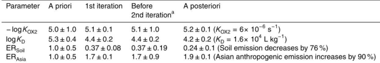
3.3 Parameter inversion

Results of the parameter inversion are presented in Table 4. The a posterioriK_OX2 of 6×10−6s−1 is much larger than its current value (1×10−7s−1) in GEOS-Chem,

sug-5

gesting that Hg0_aq dark oxidation in the ML is more important than previously thought. The a posteriori logK_D of 4.2 is lower than seawater values in the literature (Fitzger-ald et al., 2007; Batrakova et al., 2014) but agrees with the lower end of fresh water measurements (Amos et al., 2014). We attribute this discrepancy to several simplifying assumptions in GEOS-Chem.K_D is linked to the estimates of SPM concentrations in

10

the ML and organic carbon export. As described above, the amount of organic carbon export is very uncertain (5–20 Gt C yr−1). A smaller organic carbon export may corre-spond to a larger logK_D. The uncertain spatial and seasonal variations of carbon export may also affect the estimate of logK_D. In addition, there are no available global data sets of SPM in the ML. GEOS-Chem derives SPM concentrations from MODIS

satel-15

lite Chlorophyll a and C : Chl a ratios (Soerensen et al., 2010b). Thus, the uncertain SPM fields may also a_ffect logK_D. The parameter inversion decreases soil emission but increases Asian anthropogenic emission, consistent with the emission inversion.

Similar to our model–observation comparison for the emission inversion, we run GEOS-Chem using optimized parameters and calculate the NRMSEs for all

ground-20

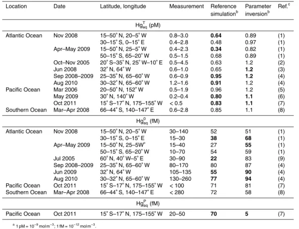
based sites (Table 1). A smaller average NRMSE of 0.14 for the parameter inver-sion than that of 0.16 for the reference simulation shows improvement in model per-formance. GEOS-Chem simulations using optimized parameters also match regional over-water Hg0(NRMSE=0.10, Fig. 2) and wet deposition measurements (Fig. S9 in the Supplement). In addition, we evaluate the optimized model against recent surface

25

ocean measurements of total aqueous mercury (HgT_aq), Hg0_aq, and HgP_aq (Table 5). For HgT_aq, 50 and 75 % (6 and 8 out of 12) modeled data from the reference and optimized

(25)

ACPD

15, 5269–5325, 2015

S. Song et al.

Title Page

Tables Figures

◭ ◮

Back Close

Full Screen / Esc

Discussion

P

a

per

|

Discussion

P

a

per

|

Discussion

P

a

per

|

Discussion

P

a

per

|

simulations, respectively, are within measurement ranges. For Hg0_aq, 60 % (6 out of 10) modeled data from both simulations are within measurement ranges. For HgP_aq, the reference simulation predicts a higher while the parameter inversion predicts a lower value than the only measurement data. These results suggest that the parameter in-version is comparable or potentially better than the reference simulation with regard to

5

modeling surface ocean mercury.

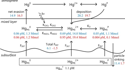
Optimizing the two ocean model parameters, −logKOX2 and logKD, changes the

global ocean Hg budget in GEOS-Chem, as shown in Fig. 6. Sources of Hg_aqin the ML include deposition of oxidized Hg and physical transport from subsurface waters. They are balanced by Hg0 evasion and HgP_aq sinking. In the reference simulation, although

10

deposition (20.2 Mmol yr−1_{) accounts for most ML Hg}

aq inputs, the two physical

trans-port processes, entrainment/detrainment of the ML and Ekman pumping, together sup-ply a considerable amount (FINT: 6.1 Mmol yr−1) from subsurface waters. This upward

flux is a result of the gradient in HgT_aq between the ML (0.8 pM) and subsurface waters (1.1 pM). Hg0evasion and HgP_aq sinking remove 14.9 and 11.4 Mmol yr−1_{from the ML,}

15

respectively. The combined effect of the larger K_OX2 and smaller K_D in the parameter inversion is, in the ML, that Hg2_aq+increases from 0.69 to 0.95 pM, HgP_aq decreases from 0.05 to 0.004 pM, and Hg0_aq remains to be 0.06 pM. HgP_aq sinking becomes a smaller sink (1.7 Mmol yr−1_{) due to the lower}_K

D. Physical transport contributes a downward flux

(−1.5 Mmol yr−1) since the gradient of HgTaq between the ML (1.0 pM) and subsurface

20

waters (1.1 pM) is diminished.

Physical transport and HgP_aqsinking a_ffect seasonal variations of simulated Hg0 eva-sion from the ocean (Soerensen et al., 2010b). In summer, enhanced biological pro-ductivity increases HgP_aqsinking and decreases Hg0evasion by shifting speciated Hg_aq equilibrium in the ML towards Hg0_aq loss. During winter months, the ML deepens and

25

(26)

ACPD

15, 5269–5325, 2015

S. Song et al.

Title Page

Tables Figures

◭ ◮

Back Close

Full Screen / Esc

Discussion

P

a

per

|

Discussion

P

a

per

|

Discussion

P

a

per

|

Discussion

P

a

per

|

transport and HgP_aq sinking are both weakened, as described above. As a result, the parameter inversion overturns seasonality of simulated ocean evasions in both hemi-spheres (Fig. 5), agreeing with results from the emission inversion.

As described in Sect. 2.6.4, we conduct an additional parameter inversion including six new elements representing Br columns in different latitudinal bands. As shown in the

5

Supplement, Fig. S8,₋logK_OX2 is found to be strongly correlated with Br columns in 30–60◦N, 30◦S–0◦, and 60–30◦S. The other three factors, logK_D, ER_Soil, and ER_Asia, have no or weak correlations with Br columns. Thus, we suggest that the inversion results of smaller terrestrial emissions and larger Asian anthropogenic emissions are not likely to be affected by the uncertainty in atmospheric chemistry, but the poor

un-10

derstanding of atmospheric chemistry may limit our ability to further constrain specific ocean model parameters.

3.4 Implications for the Hg biogeochemical cycle

We use the box model developed by Amos et al. (2013, 2014) to explore the long-term impact of our inverted emissions and parameters on the global biogeochemical cycling

15

of mercury. This seven-box model dynamically couples the atmosphere, three terres-trial reservoirs (fast, slow, and armored), and three ocean reservoirs (surface, subsur-face, and deep). All rate coefficients of Hg mass between reservoirs are assumed to be first-order. The simulation is initialized with geogenic emissions to represent natural mercury cycle, and after reaching steady state, is driven by historical anthropogenic

20

emissions (Streets et al., 2011; Horowitz et al., 2014).

Two box-model simulations are performed. The first uses rate coe_fficients from the present-day global budget in the reference simulation. The second uses those from our emission and parameter inversions, and has higher anthropogenic emissions, lower reemission from terrestrial surfaces, and less sinking out of surface ocean than the first

25

one does (Table S4 in the Supplement). The second simulation obtains larger terrestrial mercury reservoirs, highlighting their important role in sequestering legacy mercury.