ACPD
9, 22365–22406, 2009Sulfur cycle and sulfate radiative
forcing
I.-C. Tsai et al.
Title Page
Abstract Introduction
Conclusions References
Tables Figures
◭ ◮
◭ ◮
Back Close
Full Screen / Esc
Printer-friendly Version
Interactive Discussion
Atmos. Chem. Phys. Discuss., 9, 22365–22406, 2009 www.atmos-chem-phys-discuss.net/9/22365/2009/ © Author(s) 2009. This work is distributed under the Creative Commons Attribution 3.0 License.
Atmospheric Chemistry and Physics Discussions
This discussion paper is/has been under review for the journalAtmospheric Chemistry and Physics (ACP). Please refer to the corresponding final paper inACPif available.
Sulfur cycle and sulfate radiative forcing
simulated from a coupled global
climate-chemistry model
I.-C. Tsai1, J.-P. Chen1, P.-Y. Lin1, W.-C. Wang2, and I. S. A. Isaksen3
1
Department of Atmospheric Sciences, National Taiwan University, Taiwan
2
Atmospheric Sciences Research Center, State University of New York at Albany, USA
3
Department of Geosciences, University of Oslo, Norway
Received: 1 August 2009 – Accepted: 1 October 2009 – Published: 22 October 2009 Correspondence to: J.-P. Chen ([email protected])
ACPD
9, 22365–22406, 2009Sulfur cycle and sulfate radiative
forcing
I.-C. Tsai et al.
Title Page
Abstract Introduction
Conclusions References
Tables Figures
◭ ◮
◭ ◮
Back Close
Full Screen / Esc
Printer-friendly Version
Interactive Discussion
Abstract
The sulfur cycle and radiative effects of sulfate aerosol on climate are studied with a Global tropospheric Climate-Chemistry Model in which chemistry, radiation and dy-namics are fully coupled. Production and removal mechanisms of sulfate are analyzed for the conditions of natural and anthropogenic sulfur emissions. Results show that
5
the 1985 anthropogenic emission doubled the global SO2and sulfate loadings from its natural value of 0.15 and 0.27 Tg S, respectively. Under natural conditions, the fraction of sulfate produced in-cloud is 87%, and the lifetime of SO2and sulfate are 1.8 and 4.0 days, respectively; whereas with anthropogenic emissions, changes in in-cloud sulfate production are small, while SO2and sulfate lifetimes are significant reduced (1.0 and
10
2.4 days, respectively). The doubling of sulfate results in a direct radiative forcing of −0.32 and−0.14 W m−2under clear-sky and all-sky conditions, respectively, and a sig-nificant first indirect forcing of−1.69 W m−2. The first indirect forcing is sensitive to the relationship between aerosol concentration and cloud droplet number concentration. Two aspects of chemistry-climate interaction are addressed. Firstly, the coupling
ef-15
fects lead to 10% and 2% decreases in sulfate loading, respectively, for the cases of natural and anthropogenic added sulfur emissions. Secondly, only the indirect effect of sulfate aerosols yields significantly stronger signals in changes of near surface temper-ature and sulfate loading than changes due to intrinsic climate variability, while other responses to the indirect effect and all responses to the direct effect are weak.
20
1 Introduction
Aerosol particles affect the Earth’s energy budget directly by absorbing or scattering short-wave and long-wave radiation, and indirectly by influencing the structure and ra-diative properties of clouds through acting as cloud condensation nuclei and ice nuclei (Twomey, 1974; Albrecht, 1989). The perturbation of aerosols is believed to have
sig-25
ACPD
9, 22365–22406, 2009Sulfur cycle and sulfate radiative
forcing
I.-C. Tsai et al.
Title Page
Abstract Introduction
Conclusions References
Tables Figures
◭ ◮
◭ ◮
Back Close
Full Screen / Esc
Printer-friendly Version
Interactive Discussion
al., 2001; Williams et al., 2001; Rotstayn and Penner, 2001; Ramanathan, 2001; An-dersen, 2003; IPCC, 2007). Although numerous studies have estimated aerosol direct and indirect effects, the results are highly uncertain (IPCC, 2007; Lohmann, 2005). IPCC (2007) for instance, reported that the global annual mean radiative forcing of aerosol direct effect is about−0.4 W m−2 while for the first indirect effect (or the cloud
5
albedo effect) the forcing ranges from−0.3 to−1.8 W m−2.
Sulfate particle is an important component of atmospheric aerosols. Many studies have discussed the importance of the sulfur cycle (Rodhe and Isaksen, 1980; Chin et al., 1996, 2000; Feichter et al., 1996; Koch et al., 2001; Iversen and Seland, 2002; Liao et al., 2003, Berglen et al., 2004). The key species in tropospheric sulfur cycle are
10
the gaseous DMS (dimethylsufide) and SO2, and sulfate via their oxidation by various oxidants including O3, OH, H2O2, HO2NO2and NO3.
Many chemical transport models (CTMs) have been developed to simulate the sulfur cycles using prescribed (offline) meteorology to drive the chemistry. Another approach has been to use prescribed aerosol for calculating radiative forcing in global climate
15
models (e.g. Mitchell et al., 1995; Chou, 2004; Chen and Penner, 2005; Gu et al., 2006; Jones et al., 2007). Since interactions with the meteorological fields (e.g. cloud removal) are crucial to the sulfur cycle evolution, and although such simulations do include the impact of aerosol radiative forcing on atmospheric circulation, the lack of consistency in considering non-linear in situ production of sulfate aerosols (Berglen et
20
al., 2004) introduces large uncertainties in sulfur cycle estimates. Many studies indi-cated that feedbacks might be more influential than expected (Kaufman and Freaser, 1997; Cerveny and Bailing, 1998; Audiffren et al., 2004; Resenfeld, 2000), therefore, models that do not include coupled chemistry, radiation and dynamics may have large errors in the estimates of the feedback mechanisms occurring in the climate system
25
and impact the model results (Zhang, 2008).
ACPD
9, 22365–22406, 2009Sulfur cycle and sulfate radiative
forcing
I.-C. Tsai et al.
Title Page
Abstract Introduction
Conclusions References
Tables Figures
◭ ◮
◭ ◮
Back Close
Full Screen / Esc
Printer-friendly Version
Interactive Discussion
very uncertain, limited by the complexity of mechanisms considered in the model. For example, Mickley et al. (1999), considering only O3 impacts on radiation, estimated that the difference of O3 radiative forcing between offline and online calculations is about 2%. However, Shindell et al. (2001) also used online model to illustrate that the OH concentration could be reduced by about 10%, which would be significant to many
5
chemical processes.
In this study we incorporated an interactive tropospheric sulfur chemistry scheme into a global climate-chemistry model (GCCM) (Wong et al., 2004) to estimate radiative forcing of sulfate aerosols, including direct aerosol effect and aerosol-cloud albedo effect. Furthermore, by comparing simulations with and without the coupling of aerosol
10
radiative forcing, we examined the meteorological responses to the forcing as well as feedbacks to the meteorology and subsequently to the aerosol fields.
2 Description of the model and the simulations
2.1 Global climate-chemistry model
The GCCM was developed by incorporating the University of Oslo tropospheric
pho-15
tochemical scheme (Isaksen and Hov, 1987; Berntsen and Isaksen, 1997) into the National Center for Atmospheric Research Community Climate Model (CCM3) with modification by the group of State University of New York at Albany (Wang et al., 1995; Wong and Wang, 2000, 2003). This model has been used for simulating tropospheric chemistry and the effect of ozone on radiation. In spite of cold biases of about 4–12 K
20
in the polar regions, and small dry biases during July to August in Northern Hemi-spheric mid-latitudes, this model can reproduce reasonable inter-annual variability of the tropospheric system (Hack et al., 1998; Wong and Wang, 2003).
However, in Wong et al. (2004) the sulfur chemistry that is important for the study of aerosol effects was not included because their focus was on ozone and its impact.
25
ACPD
9, 22365–22406, 2009Sulfur cycle and sulfate radiative
forcing
I.-C. Tsai et al.
Title Page
Abstract Introduction
Conclusions References
Tables Figures
◭ ◮
◭ ◮
Back Close
Full Screen / Esc
Printer-friendly Version
Interactive Discussion
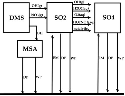
(2004) into GCCM, to take into account the interaction with the sulfate chemistry. Per-forming on-line calculations provide consistent estimates of chemical distribution and changes of gaseous- and aqueous-phase compounds. Four new species, DMS, SO2, MSA and SO24− (sulfate), are added. The new processes considered are: emission of SO2, DMS and SO24−, dry and wet deposition of SO2, MSA and SO24−, and
gaseous-5
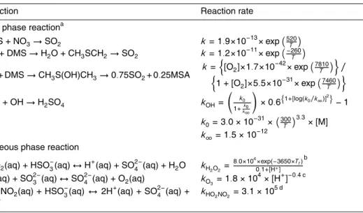
and aqueous-phase chemical reactions, as shown in the schematics of Fig. 1. The key gas and aqueous phase reactions for the sulfur cycle are listed in Table 1, and more details can be found in Berglen et al. (2004). Note that in the GCCM sea-surface temperatures are specified according to the results from the Atmospheric Model Inter-comparison Project 2 (AMIP 2) (Gates et al., 1999).
10
2.2 Emissions
The global emissions of pollutants except sulfur species are based on IPCC 2001 (Ox-Comp Y2001), with annual mean values rescaled to 1990 emission following Wong et al. (2004). Sulfur emissions include anthropogenic emission sources following the GEIA 1985 inventory (Benkovitz et al., 1996), ship emission from Endresen et al.
15
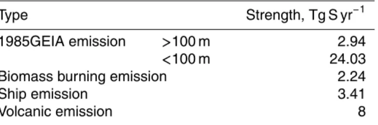
(2003), biomass burning from Spiro et al. (1992) and Graft et al. (1997). Table 2 shows the total emission strengths from each source. It is assumed that 5% of anthropogenic sulfur is emitted as sulfates while the rest as SO2(Langner and Rodhe, 1991).
Natural sulfur sources include volcanic emission (Spiro et al., 1992) and DMS emis-sion from the ocean (Kettle et al., 1999; Kettle and Andreae, 2000). The DMS flux is
20
calculated with specified seawater DMS concentrations using transport parameteriza-tion of Liss and Merlivat (1986):
F =Vk×(CDMS,air/H−CDMS,ocean) (1)
whereVk is parameterized transport velocity, CDMS,air is DMS concentration in air, H
is Henry constant for DMS, and CDMS,ocean is DMS concentration in seawater. The
25
ACPD
9, 22365–22406, 2009Sulfur cycle and sulfate radiative
forcing
I.-C. Tsai et al.
Title Page
Abstract Introduction
Conclusions References
Tables Figures
◭ ◮
◭ ◮
Back Close
Full Screen / Esc
Printer-friendly Version
Interactive Discussion
in this study (based on the assumptions made for the products in Reaction (R3) in Table 1).
2.3 Cloud effective radius
As mentioned in previous sections, the sulfate particles could serve as cloud con-densation nuclei and modify cloud drop number concentration hence cloud radiative
5
properties, leading to the cloud albedo effect. However, similar to that done in many other GCMs, the previous version of GCCM applies prescribed cloud droplet effective radii of 5µm over continents and 10µm over oceans for the radiation calculation. Such an approach only grossly represents the spatial distribution of aerosol influences and certainly cannot reflect response to the change of aerosols. Based on observations,
10
Boucher and Lohmann (1995) provided improvement with empirical formulas that link the effective radii of cloud drops to sulfate mass loading:
NC =exp(a0+a1∗log(MSO4)) (2)
whereMSO4 is the sulfate mass loading inµg/m−3andNC is the cloud droplet number
concentration in cm−3, and different values of coefficientsa0anda1are provided for the
15
continental and oceanic conditions. However, their formulas tend to overestimate the number concentration of cloud drops, thus underestimate the effective radii, especially over the oceans. That will lead to overestimated sulfate radiative forcing. Quaas and Boucher (2005) made an adjustment to correct for this underestimate and provided the coefficientsa0=3.9 anda1=0.2, and these are the values adopted for this study. The
20
coefficients given by Boucher and Lohmann (1995) will also be tested and presented in the discussion section. The effective radiusre can be calculated as:
re=
3w l
4πρwkNc
1/3
(3)
ACPD
9, 22365–22406, 2009Sulfur cycle and sulfate radiative
forcing
I.-C. Tsai et al.
Title Page
Abstract Introduction
Conclusions References
Tables Figures
◭ ◮
◭ ◮
Back Close
Full Screen / Esc
Printer-friendly Version
Interactive Discussion
cloud droplets, which is assumed as 0.67 over continents and 0.8 over oceans accord-ing to Martin et al. (1994).
2.4 Simulations
Two sets of simulations are conducted to estimate the sulfate aerosols direct and indi-rect effects. Simulations N0, N1 and N2 apply only natural sulfur emissions (i.e. DMS
5
and volcanic SO2 emissions), whereas simulations A0, A1 and A2 take additional an-thropogenic sulfur emissions. The degree of coupling the aerosol effects is indicated by the numbers after “N” and “A”, where “0” denotes no sulfate radiative effects, “1” de-notes only sulfate direct effect, and “2” indicates both sulfate direct effect and the first indirect effect. Six months spin-offwere conducted for N0, and then used to run other
10
cases for a period of 13 years. For analysis, we used results from the last 5 years. Monthly meteorological fields and trace gas concentrations were examined to ensure that near-steady-state climate conditions are reached.
All simulations apply a horizontal resolution of T42 (equivalent to 2.8◦×2.8◦) and 18 vertical layers from the surface to about 2.5 hPa. The time step used is 20 min, with the
15
exception that shortwave and long-wave radiation processes are calculated hourly.
3 Analyses
In the following we first briefly compare the global distribution of simulated meteoro-logical fields and sulfur species with observational data to check the general model performance using results from the A2 and N2 simulations. Next, sulfate aerosol
forc-20
ing as well as the effect of coupling will be discussed for the simulations.
3.1 Global distributions
temper-ACPD
9, 22365–22406, 2009Sulfur cycle and sulfate radiative
forcing
I.-C. Tsai et al.
Title Page
Abstract Introduction
Conclusions References
Tables Figures
◭ ◮
◭ ◮
Back Close
Full Screen / Esc
Printer-friendly Version
Interactive Discussion
ature and wind fields are compared with the 1979–2005 climatology of the NCEP-DOE Reanalysis 2 (NCEP RE2), whereas surface precipitation is compared with that of the Global Precipitation Climatology Project (GPCP, 1979–present). Figure 2a–d show the convergence over tropical regions, divergence over 30◦N and 30◦S and the distribution of isothermal of A2 results are similar to NCEP RE2 climatology. The pattern of surface
5
precipitation simulated with GCCM is generally quite similar to those of GPCP, except that the model result is wetter over the tropics and drier over mid-latitude Pacific Ocean (Fig. 2e and f). Since the model sea surface temperature is prescribed, air temperature above the ocean is close to the climatology.
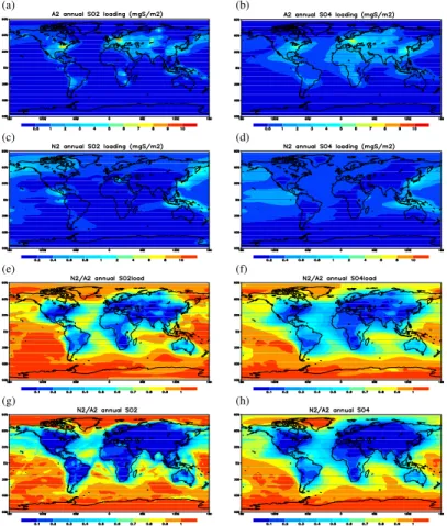
Figure 3a shows the simulated global distribution of SO2column concentration from
10
simulation A2. Note that areas of high concentrations near or downwind of major an-thropogenic emission hot spots occur in central Europe, eastern United States, eastern China, and Russia. There are also secondary maxima in southern Africa, South Amer-ica and Indonesia due to biomass burning and volcanic eruptions. These patterns are in general agreement with GOME satellite observation reported in Khokhor et al.
15
(2004). Differences exist in a few places, partly because the 1985 distribution is for a different time period than the GOME observations, for which data are available only after 1995. Besides the differences in anthropogenic emission inventory, the discrep-ancies may also result from the use of climatological volcanic emissions in our simula-tions, which might not reflect major volcanic eruptions during 1996–2002 (Khokhor et
20
al., 2004). Nevertheless, the GCCM simulation captured the general features of SO2 spatial distribution.
The sulfate distribution has a rather similar pattern as SO2 (Fig. 3b), except that it spreads over a wider area, likely due to time lag of chemical conversion from SO2which allows more time for atmospheric dispersion, since it is a secondary compound, while
25
ACPD
9, 22365–22406, 2009Sulfur cycle and sulfate radiative
forcing
I.-C. Tsai et al.
Title Page
Abstract Introduction
Conclusions References
Tables Figures
◭ ◮
◭ ◮
Back Close
Full Screen / Esc
Printer-friendly Version
Interactive Discussion
so their global features can be distinctly different from the sulfate distribution. Another way to check the correctness of our sulfur-cycle calculations is to compare with results from other models that also applied the 1985 emission inventory. Global model studies referred to in Berglen et al. (2004) and in the AeroCom project (Schulz et al., 2006) revealed large differences in current estimates of sulfate burden. The mean global
5
loading of SO2and sulfate from our A2 simulation are 0.29 and 0.54 Tg S, respectively, as listed in Table 3. These global loadings are on the low side but within the range of other model results.
In the following discussion we analyze the contribution of sulfur species from different emission sources and the production mechanisms of sulfate. The natural SO2
concen-10
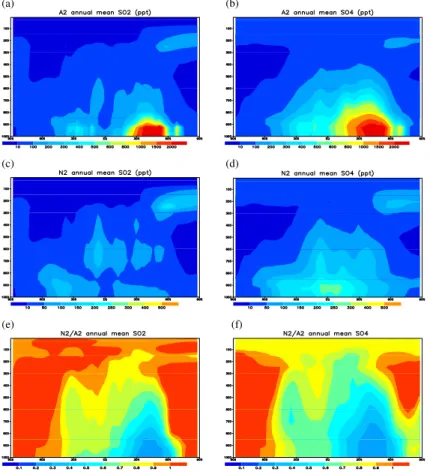
trated over the northern high latitudes and tropical regions to the east of Indonesia (Fig. 3c) are mainly from volcanic emissions. Annual global production of SO2 from DMS is about 21.8 Tg S, much higher than the 8 Tg S per year from volcanic emissions (Table 2). However, DMS is released in the lower troposphere, so the SO2formed from DMS may experience stronger surface removal by dry deposition or conversion to
sul-15
fate by aqueous-phase reactions where liquid clouds are prevalent. Volcanic emission is actually a more dominant source of global SO2, typically injected into the upper tro-posphere (Fig. 4c). Thus, the global distribution of column SO2in Fig. 3c does not show obvious signature of DMS production zones but rather concentrate over the volcanic active areas. But from the vertical distribution shown in Fig. 4c one may notice the
20
presence of DMS-converted SO2that stays near the surface over mid-latitude oceans (mainly around 40◦S and some over 10–60◦N).
Natural sulfate also spreads over a much wider area than SO2distribution (Fig. 3d). This feature can also be seen in the vertical distributions in Fig. 4d. Figure 3e gives the ratio of natural to total SO2(N2 to A2), and from it one can see that anthropogenic
25
ACPD
9, 22365–22406, 2009Sulfur cycle and sulfate radiative
forcing
I.-C. Tsai et al.
Title Page
Abstract Introduction
Conclusions References
Tables Figures
◭ ◮
◭ ◮
Back Close
Full Screen / Esc
Printer-friendly Version
Interactive Discussion
dominating only over the polar regions and some remote oceans. The contrast of nat-ural versus anthropogenic contributions of SO2 is even sharper at the surface layer. Figure 3g show that more than 90% of the surface SO2 over most of the land areas is of anthropogenic origin. Over the remote oceans one can see the dominance of anthropogenic emissions on SO2 concentration over major shipping routes. But the
5
surface distribution of sulfate (Fig. 3h) does not retain the features of shipping cor-ridors, again indicating the time lag in SO2 to sulfate conversion and more efficient sulfate dispersion.
The vertical distribution of sulfur depends on the location of emission sources as well atmospheric transport and removal processes. As shown in Fig. 4e and f, the fraction
10
of anthropogenic SO2over mid-latitude Northern Hemisphere exceeds 90% near the surface, and the value remains above 50% up to the 500-hPa level. In the Southern Hemisphere, the highest anthropogenic fraction is at the surface around 20◦S, while the 50% isopleth stays below the 900-hPa level. Fraction of sulfate from anthropogenic contributions generally exceeds that of SO2. As shown in Fig. 4f, the 50% isopleths
en-15
close a large portion of the troposphere and may reach an altitude of 200 and 400 hPa over the Northern and Southern Hemisphere, respectively. Globally, natural emissions are responsible for slightly more than one half of the total for both sulfur species (see Table 3).
The net sulfate loading is determined by the rates of production (direct emission and
20
oxidation from SO2 in air and clouds) and removal (dry and wet deposition). A brief overview of the magnitude of each process may facilitate the discussion of the cou-pling effect in later sections. According to the N2 simulation, annual production of SO2 is 29.8 Tg S (including volcanic emission and conversion from DMS), whereas under polluted condition (A2) the total production is 102.4 Tg S. Conversion of SO2into
sul-25
ACPD
9, 22365–22406, 2009Sulfur cycle and sulfate radiative
forcing
I.-C. Tsai et al.
Title Page
Abstract Introduction
Conclusions References
Tables Figures
◭ ◮
◭ ◮
Back Close
Full Screen / Esc
Printer-friendly Version
Interactive Discussion
11% by OH. Such a change of proportions indicates that the increase of tropospheric ozone due to human pollution significantly enhances in-cloud production of sulfate. The concentration of H2O2 and OH also increased somewhat, leading to enhancement of sulfate production both by 2.8 folds. But such an enhancement is actually less than the 3.4 times increase of SO2productions (A2 versus N2), and this implies that H2O2and
5
OH are probably the predominant limiting agent in the oxidation reactions. On the other hand, the enhancement of sulfate production by ozone oxidation (3.6 times) is close to that of SO2 production, indicating that ozone is usually not the limiting agent. The fraction of in-cloud sulfate production from our A2 results (89%) is significantly higher than in several global CTMs. For example, the values estimated by Chin et al. (2000),
10
Restad et al. (1998), Koch et al. (1999) and Roelofs et al. (1998) range from 64 to 78%. However, our value is closer to the 84 to 85% by Berglen et al. (2004) and Chin et al. (1996). It is also similar to the 86% in Lelieveld (1993) who performed the estimation based on global cloud climatology and specified chemical reaction rates. As GCCM applied essentially the same chemical scheme as Berglen et al. (2004), the
discrep-15
ancy between them is likely due to differences in meteorology, such as the amount of liquid cloud and transport processes. Under natural conditions, the removal of sulfate from the atmosphere is mainly via wet deposition, and only 7.7% is by dry deposition. For polluted conditions, the proportion by dry deposition increases to 9.4%, since most of the anthropogenic SO2 are emitted close to the surface, so they are more
suscep-20
tible to dry deposition than natural emissions from volcanic eruptions and secondary SO2from DMS.
Dividing the global loading given in Table 3 by the overall rate of destruction (same as rate of production under steady state), we are able to estimate the lifetime of SO2, which is 1.8 days under natural conditions (N2), and 1.0 days under polluted conditions
25
unpol-ACPD
9, 22365–22406, 2009Sulfur cycle and sulfate radiative
forcing
I.-C. Tsai et al.
Title Page
Abstract Introduction
Conclusions References
Tables Figures
◭ ◮
◭ ◮
Back Close
Full Screen / Esc
Printer-friendly Version
Interactive Discussion
luted (N2) and polluted (A2) conditions. Sulfate lifetime from A2 is significantly lower than from the aforementioned CTM calculations, which range from 3.7 to 5.7 days. The overall lifetime of sulfur (SO2plus sulfate) is 5.3 days in N2 and 2.9 days in A2.
The atmospheric lifetime is determined by its largest sink, so for SO2 the dominat-ing factor is in-cloud oxidation, while for sulfate wet deposition is the most important.
5
The large variation of sulfur lifetime among models shown above indicates high un-certainties in the simulation of sulfur cycle, and the unun-certainties are mainly a result of differences in formulating cloud-related sink processes. As mentioned previously, the in-cloud oxidation of SO2 in GCCM is stronger than in other models, so it is not surprising that our calculation of SO2lifetime is shorter. Furthermore, this also implies
10
that the amount of cloudwater (for the oxidation to take place) could be quite diff er-ent among models. Apparer-ently, different climate models, even with prognostic clouds, cannot get consistent cloud water and precipitation (cf. Lau et al., 1996). A stronger in-cloud production also means a shorter lifetime for sulfate (larger production rate), which partly explain why the value from our model is significantly lower. The shorter
15
lifetime of sulfate could also mean a stronger precipitation which lead to stronger wet deposition. Again, precipitation among climate models are very different, and the value (3.2 mm day−1) obtained in GCCM is on the high side compared to various GCM re-sults from AMIP (Lau et al., 1996). We find that the coupling of sulfate radiative forcing, which will be discussed later, caused a reduction of mass loading hence shortened the
20
lifetime of sulfate, and the reduction is about 10% for the natural conditions (N2 versus N0) and 2% for the polluted conditions (A2 versus A0). From budget analysis we found that the reduction of sulfate loading in A2 versus A0 is due to a stronger wet deposi-tion, which is related to the stronger precipitation (see Table 5), as well as a weaker aqueous-phase production, which is a consequence of lower SO2 concentration (see
25
distri-ACPD
9, 22365–22406, 2009Sulfur cycle and sulfate radiative
forcing
I.-C. Tsai et al.
Title Page
Abstract Introduction
Conclusions References
Tables Figures
◭ ◮
◭ ◮
Back Close
Full Screen / Esc
Printer-friendly Version
Interactive Discussion
butions and variation of oxidants (e.g. O3, OH), which are responsible for atmospheric conversion of SO2to sulfate are similar to what was presented by Wong et al. (2004).
3.2 Sulfate radiative forcing
In this section we present the direct effect and the first indirect effect of sulfate aerosol forcing. To determine radiative forcing from anthropogenic sulfate aerosols, we simply
5
take the difference between the A-series and N-series calculations. The distribution of radiative forcing at the surface is very similar to the distribution at the top of the atmosphere (TOA), only the latter is therefore discussed.
Direct forcing for both clear-sky and all-sky conditions can be obtained from either the A1–N1 or the A2–N2 results. Note that sulfate in A0 and N0 does not affect
radi-10
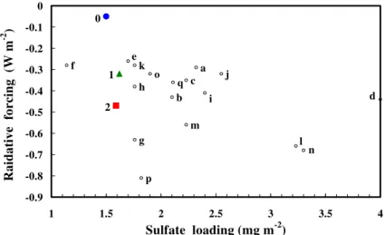
ation, so the differences of radiative forcing between these two simulations arise from the influences of ozone chemistry and from model internal variability, which will be further elaborated later. Globally, as shown in Table 4, aerosol direct forcing is about −0.32 W m−2 at TOA, which is more significant than the −0.05 W m−2 by ozone from the A0–N0 results. Figure 5 compares the mass loading and direct forcing of sulfate
15
from various models, and the values from GCCM are well within the range of others. Direct forcing under all-sky conditions may be represented by the A1–N1 forcing, as neither A1 nor N1 considered the sulfate indirect effect. From Table 4 we can see that the global direct forcing reduces to−0.14 W m−2for all-sky conditions.
For the indirect forcing of anthropogenic sulfate, it may be represented by the
dif-20
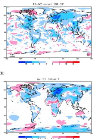
ferences between the A2 and N2 results. Note that, because the cloud effective radii are prescribed in A0, A1, N0 and N1 simulations, it is not appropriate to use A2–A0 or N2–N0 to represent the indirect effect of sulfate. Figure 6a shows the distribution of total sulfate forcing based on A2–N2 results. As the indirect forcing is much higher than the direct forcing (see Table 4), one may regard them as all from the indirect effect.
25
forc-ACPD
9, 22365–22406, 2009Sulfur cycle and sulfate radiative
forcing
I.-C. Tsai et al.
Title Page
Abstract Introduction
Conclusions References
Tables Figures
◭ ◮
◭ ◮
Back Close
Full Screen / Esc
Printer-friendly Version
Interactive Discussion
ing may reach−20 W m−2 over eastern North America and southeastern China. But there are also areas experiencing positive forcing, mostly over the continents around the regions of strong negative forcing, possibly resulting from regional adjustment in the dynamics and cloud fields. These positive forcing leads to a smaller global indirect forcing that averages to about−1.69 W m−2. Similar to the approach applied earlier,
al-5
ternative estimation can be derived by deducting the N2–N0 forcing from that of A2–A0 for all-sky conditions, which gives a global indirect forcing of−1.56 W m−2. This value is rather close to that from the A2–N2 results, indicating the robustness of its value.
To provide a broader perspective, we compare our model results with other studies, noting that there are many differences among the models. IPCC (2007) summarized
10
results from different estimations and suggested the range of −0.1 to −0.9 W m−2 for the direct effect, and−0.3 to−1.8 W m−2 for the first indirect effect. Our estimation of the direct effect is within the range and the indirect effect is on the high end. However, our simulations consider only sulfate aerosols, while some of those reported in IPCC (2007) may contain other aerosol types.
15
3.3 Climate responses to sulfate forcing
Aerosol forcing affects the energy budget thus the dynamics of the atmosphere, which in turn influence clouds and precipitation then consequently the feedback to the radia-tion field. Figure 6b shows the changes in near-surface air temperature due to direct and indirect forcing according to the results of A2–N2. Significant cooling can be found
20
over (but not confined to) the three main areas of pollution sources: eastern China, Eastern Europe, and eastern United States. One can also find significant warming over areas such as northern North America, mid-north Africa, and northern Australia. The temperature change pattern does not have a one-to-one correspondence with the pattern of radiative forcing that is shown in Fig. 6a, indicating that the radiation field
25
has interactions with the dynamic and cloud fields.
ACPD
9, 22365–22406, 2009Sulfur cycle and sulfate radiative
forcing
I.-C. Tsai et al.
Title Page
Abstract Introduction
Conclusions References
Tables Figures
◭ ◮
◭ ◮
Back Close
Full Screen / Esc
Printer-friendly Version
Interactive Discussion
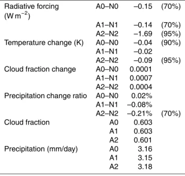
Table 5. The direct forcing (A1–N1) leads to a decrease of global near-surface air tem-perature by about 0.02 K, but this change is even smaller than the−0.04 K forcing from ozone changes estimated from the A0–N0 results. This indicates that the direct forcing is probably too weak compared to other forcing mechanisms. On the other hand, the 0.09 K cooling due to both the direct and indirect effects (A2–N2) is larger than that
5
from A1–N1, and apparently most of it is from the indirect effect. Note that the change in surface air temperature here is underestimated because of the fixed ocean surface temperature. The indirect effect of anthropogenic sulfate also leads to an increase of cloud coverage by 0.04% and a depression of precipitation by 0.21% due to dynamic feedbacks. The contrasting change in cloud coverage and precipitation implies that the
10
additional clouds are mostly non-precipitating type. But these small changes are prob-ably not particularly meaningful when considering the internal variability of the model as will be discussed later. The responses of global mean cloud amount due to the di-rect forcing of sulfate (A1–N1) are more significant even thought the forcing is weaker as compared with the indirect forcing.
15
The GCCM responses to sulfate forcing are more significant on the regional scale and may even lead to changes in the monsoon system. In East Asia for example, weaker summer monsoon and stronger winter monsoon emerge under the forcing of anthropogenic sulfate, leading to reduced moisture flux from the ocean to the East Asian continent in both seasons. The changes are in many aspects similar to those
20
simulated with the regional coupled climate-chemistry model by Huang et al. (2007) who found a regional radiative forcing of−4.08 W m−2, leading to a cooling of the mean surface temperature by 0.35 K and reduced cloud fraction by 0.8% and precipitation by more than 10%; whereas the values we obtained are−3.99 W m−2,−0.24 K,−1%, and −5.3%, respectively. In addition, the two simulation results share similar geographic
25
ACPD
9, 22365–22406, 2009Sulfur cycle and sulfate radiative
forcing
I.-C. Tsai et al.
Title Page
Abstract Introduction
Conclusions References
Tables Figures
◭ ◮
◭ ◮
Back Close
Full Screen / Esc
Printer-friendly Version
Interactive Discussion
with assimilated aerosols. In other regions the responses to sulfate forcing may be quite different, and the details are quite convoluted and tedious thus will not be elaborated here.
3.4 Effect of coupling on sulfate chemistry
The climate responses discussed above will also alter the transformation, transport,
5
and removal of aerosols, thus forming feedback loops. Because atmospheric sulfate is formed mainly in liquid clouds (about 89% in A2), while its removal is mainly by precipi-tation scavenging (about 75% in A2), any change in the cloud fields could affect sulfate loading. In addition, the changes in circulation and other parameters such as humidity and actinic flux due to sulfate forcing may influence the transport, dry deposition as well
10
as chemical formation of sulfate. These feedbacks exist only when the sulfur chemistry is coupled to processes in the climate model.
However, to examine the sensitivity of the sulfur cycle to sulfate forcing, it is not proper to compare simulation set of A2–N2 (or A1–N1, A0–N0) as done earlier, be-cause it would only reflect the large differences in emissions. A better comparison can
15
be performed between either the A-series or N-series of simulations, as their emissions are the same but the degrees of coupling of sulfate forcing are different. Note that A0 and A1 simulations do include cloud forcing but the calculations are based on specified effective radii. From Table 3 we can see that SO2loading remains quite steady among the N-series of simulations, and varies only slightly among the A-series of simulations.
20
Sulfate loading under natural conditions varies more significantly, with the N2 sulfate loading being 10% less than that from N0. Under polluted conditions, sulfate calcu-lated with the fully-coupled A2 simulation (0.54 Tg S) is only about 2% less than that (0.55 Tg S) from the less coupled simulations (i.e. A1 and A0). The main cause of these differences in sulfate loading is the change in dry deposition, which should be related to
25
ACPD
9, 22365–22406, 2009Sulfur cycle and sulfate radiative
forcing
I.-C. Tsai et al.
Title Page
Abstract Introduction
Conclusions References
Tables Figures
◭ ◮
◭ ◮
Back Close
Full Screen / Esc
Printer-friendly Version
Interactive Discussion
precipitation in N0) as well as decreased conversion from SO2 oxidation. However, these reductions may be too small to cause significant feedbacks to radiative forcing.
4 Discussions
Earlier we showed that sulfate aerosols may exert forcing on several climate parame-ters including surface temperature, winds, clouds and precipitation. The indirect forcing
5
due to cloud albedo effect seems to be quite significant from the fully coupled A2–N2 results. However, as indicated from the A1–N1 results, the direct forcing of anthro-pogenic sulfate is so weak that its signal might not be distinguishable from other ef-fects that have similar or greater magnitudes. For example, the change of gas-phase chemistry (i.e. increasing ozone) due to anthropogenic pollutants could induce similar
10
temperature change as indicated by the A0–N0 results where aerosol forcing is not considered. It is important to establish whether the climate responses we saw in the previous section are truly from the aerosol effects or simply noises. Nevertheless, the A2–N2 results do show a strong signal of responses to the indirect forcing by sulfate, even though the results do contain uncertainties as discussed in the following.
15
To eliminate the possibility that differences between simulations shown in Tables 4 and 5 simply are due to internal climate variability of the model, we need to understand how large such an internal variability is. In Fig. 7 the response of several parameters is plotted against their internal variability. The response is defined as the difference between two sets of simulations, whereas the internal variability is defined as the
sea-20
sonal or annual anomaly during the 5 years of simulation time using the second set of simulation as the reference. For example, with the mean temperature difference of A2– N2 as the response, the deviation of annual mean temperature of the subtrahend, N2, from their 5-year average will represent the internal variability. Note that in the above example one may also choose the A2 results to represent the internal variability, and
25
ACPD
9, 22365–22406, 2009Sulfur cycle and sulfate radiative
forcing
I.-C. Tsai et al.
Title Page
Abstract Introduction
Conclusions References
Tables Figures
◭ ◮
◭ ◮
Back Close
Full Screen / Esc
Printer-friendly Version
Interactive Discussion
that the responses of TOA radiation to sulfate indirect forcing (A2–N2) lies consistently between−1.5 and−2.0 W m−2, and they are significantly larger than the internal vari-ability which lies within±0.2 W m−2. But for the ozone forcing (A0–N0) or the sulfate direct forcing (A1–N1) the responses are of similar magnitude as the internal variability. Furthermore, the spread across the one-to-one line indicates they are not consistently
5
larger or smaller than the internal variations. These features are consistent with their statistical significance listed in Table 5, with only the A2–N2 forcing reaching the 95% confidence level. The responses of near-surface temperature (Fig. 7b) to ozone forc-ing and, in particular, to sulfate direct forcforc-ing are again not significant; whereas the responses to indirect forcing of A2–N2 are distinctly larger than the internal
variabil-10
ity (within 0.04 K) except one data point, for which year the near-surface temperature still decreases but the amplitude is too small to be regarded as significant. This out-lier lowered the certainty of temperature responses, but the statistical significance still reached 95% (Table 5). The responses in cloud fraction and precipitation change are all indistinguishable from the internal variability, thus their statistical significance are
15
low. Note that the internal variability in shortwave radiation and surface temperature from simulations of the A-series are a bit smaller than from N-series, so the above discussion is based on a stricter standard.
Sulfate itself also responds to the forcing it created, such as changes in circulation and transport patterns, as well as in-cloud chemical production and rain scavenging.
20
As mentioned before, for such feedbacks we need to compare the results of A2–A0 (or A2–A1) instead of A2–N2 or A1–N1. Figure 7c shows that A2–A0, A2–A1, N2–N0 and N2–N1 give responses in sulfate loading consistently on the negative side (the behavior of A2–A1 is quite similar to that of A2–A1 thus are not shown). However, the annual variability of sulfate loading in N0 may sometimes exceed the responses
25
ACPD
9, 22365–22406, 2009Sulfur cycle and sulfate radiative
forcing
I.-C. Tsai et al.
Title Page
Abstract Introduction
Conclusions References
Tables Figures
◭ ◮
◭ ◮
Back Close
Full Screen / Esc
Printer-friendly Version
Interactive Discussion
progressively to ±0.04 for A0, ±0.03 for A1, and ±0.02 for both A2 and N2. So, if we take the minuend (e.g., N2 in N2–N0) as the reference instead, the responses from N2–N0 would also be regarded as distinctly evident. The magnitude of annual variations seems to decrease with the degree of complexity in the simulation (e.g., with anthropogenic emissions, or with coupled direct or indirect effects). In other words,
5
more controlling mechanisms may lead to a more stable sulfate loading. But the same does not apply to the internal variability of near-surface temperature, cloud fraction and precipitation, which remain similar among the simulations.
Another model uncertainty originates from the treatment of cloud drop effective radii. Recall that the A0 and N0 simulations applied prescribed cloud effective radii, with
10
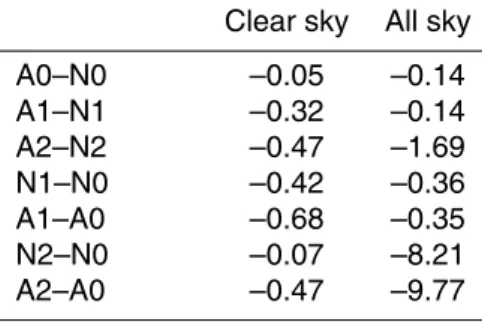
10µm over the ocean and 5µm over the continent. Such a treatment gives radia-tive forcing very different from that calculated through the empirical formula (2). As can be seen from Table 4, the difference in all-sky radiation between N2 and N0 (A2 and A0) may reach 8.2(9.8) W m−2, which is much stronger than the indirect forcing of −1.69 W m−2that discussed earlier. Such differences do contain contributions from the
15
direct aerosol forcing, but the effect should be small as can be seen from the clear-sky values. This implies that the model result is sensitive to the treatment of cloud drop effective radius and warrant the use of a more sophisticated scheme than using fixed values of 5 or 10µm. Figure 8 shows the differences between results using the empiri-cal formula and those with fixed effective radii. One can see that Eq. (2) gives stronger
20
cloud forcing over the oceans but weaker forcing over most of the continents except the highly polluted area such as northeastern US and Europe in Fig. 8b. Therefore, the size range of effective radii across the continent and ocean is smaller than the specified range of 5 to 10µm in N0 and A0, and this seems to be too narrow. We found that the inferred effective radii are still not much less than 5µm even over polluted regions.
Fur-25
ACPD
9, 22365–22406, 2009Sulfur cycle and sulfate radiative
forcing
I.-C. Tsai et al.
Title Page
Abstract Introduction
Conclusions References
Tables Figures
◭ ◮
◭ ◮
Back Close
Full Screen / Esc
Printer-friendly Version
Interactive Discussion
between sulfur loading and effective radius.
The original coefficients for Eq. (2) from Boucher and Lohmann (1995) give much stronger dependences of cloud-drop number concentration on sulfate loading. When we apply them for the calculations in A2 and N2 (hereafter named A2B and N2B), the differences in cloud forcing indeed become obvious also over the polluted continents
5
(Fig. 8d), while those for natural conditions in Fig. 8c remain similar in spatial distribu-tion but lower in magnitude than those using the adjusted coefficients in Fig. 8a as they should be. However, the global sulfate forcing (A2B–N2B) now becomes−6.7 W m−2, which is much too high as compared with the estimations given in ICCP (2007). So, it is troublesome that the observation-based and seemly more reasonable relationship
10
between drop number and sulfate loading from Boucher and Lohmann (1995) overesti-mate the sulfate indirect forcing, whereas the relationship of Quass and Boucher (2005) that constrained total forcing (to give reasonable results) does not produce reasonable variations in effective radii. One possible explanation is that the incoming shortwave radiation sees mainly the cloud top, not deep inside the cloud or near the cloud base
15
where the measurements of sulfate loading and cloud drop number were performed. Due to various number-reduction processes (such as coalescence, accretion or evap-oration due to Bergeron-Findeisen conversion or entrainment mixing), the number of cloud drops tends to vary significantly with height. The microphysical properties near the top of clouds (particularly those high enough to be glaciated partly or fully) might
20
not respond significantly to the change in sulfate loading. It is also possible that Eq. (2) is an oversimplification, as the cloud-drop number concentration actually depends on the size spectrum and chemical composition of the aerosol particles in addition to the strength of updraft. As both the constrained and un-constrained sulfate-effective-radius relationships may contain large uncertainties, more detailed treatment of aerosol-cloud
25
ACPD
9, 22365–22406, 2009Sulfur cycle and sulfate radiative
forcing
I.-C. Tsai et al.
Title Page
Abstract Introduction
Conclusions References
Tables Figures
◭ ◮
◭ ◮
Back Close
Full Screen / Esc
Printer-friendly Version
Interactive Discussion
5 Conclusions
In this study, we incorporated a sulfur cycle scheme that interact on-line with an ex-tensive gas phase scheme previously included, to take into account emissions, gas-and liquid phase chemical processes, gas-and deposition processes, into a Global Climate-Chemistry Model to study the sulfur cycle and the effect of sulfate aerosols on climate
5
through scattering of solar radiation and change of cloud albedo. The coupling of aerosol and cloud radiation with the meteorology also allowed us to analyze response of the climate parameters and their feedback.
Under pre-industrial natural conditions, over 73% of the atmospheric SO2 is pro-duced by DMS oxidation, the rest by volcanic activities. Whereas 87% of SO2 is
con-10
verted to sulfate in the atmosphere, nearly all of the rest is removed by dry deposition. Sulfate is produced mainly by in-cloud oxidation (51% with ozone and 34% with H2O2), and 92% of it is removed by wet deposition. Adding the 1985 anthropogenic emission, which accounts for 79% of the total SO2production, global burden of SO2and sulfate both nearly doubled. About 80% of SO2 convert to sulfate, and the weighting of
sul-15
fate production by in-cloud ozone oxidation increases to 56%, while the fractions by H2O2 oxidation and gas-phase OH reaction decrease to 30% and 11%, respectively. Wet deposition is still the dominating sink for sulfate, accounting for 91% of the loss. Atmospheric lifetimes of SO2and sulfate calculated from GCCM are 1.8 and 4.0 days, respectively, under natural conditions. The values become 1.0 and 2.4 days when
an-20
thropogenic emissions are included. The overall lifetime of sulfur (SO2 plus sulfate) is 5.3 days for natural conditions and 2.9 days with anthropogenic emission. Due to its rather short lifetime, anthropogenic SO2stays mostly over the populated continents and the nearby oceans, as well as over the shipping corridors. Being a secondary compound and the more than doubled lifetime allows sulfate to disperse further
down-25
ACPD
9, 22365–22406, 2009Sulfur cycle and sulfate radiative
forcing
I.-C. Tsai et al.
Title Page
Abstract Introduction
Conclusions References
Tables Figures
◭ ◮
◭ ◮
Back Close
Full Screen / Esc
Printer-friendly Version
Interactive Discussion
Anthropogenic SO2, on the other hand, shows its dominance only below the 500 hPa level over the pollution sources.
With the 1985 emissions, global mean sulfate burden increased from the natural condition of 0.27 to 0.54 Tg S. The increase of sulfate may cause a reduction of global incoming solar radiation by about 0.47 W m−2from the direct scattering (under all-sky
5
conditions), and by 1.69 W m−2from the enhancement of cloud albedo. Such radiative forcing may cause global mean temperature to decrease by a meager 0.02 and 0.09 K, respectively. Other climate parameters also seem to respond vaguely to sulfate forcing, such as the slight increase in global cloud fraction and reduction of global precipitation. Regional radiative forcing and temperature response can be much higher, reaching
10
−7 W m−2 and −0.6 K in Europe, −4 W m−2 and −0.2 K in East Asia, and −5 W m−2 and −0.2 K in North America, but the responses in clouds and precipitation can be quite different from the global mean, such as increasing cloudiness in Europe and North America but increasing clear sky in East Asia.
By designing a series of simulations that turn on and offthe anthropogenic emissions
15
or the aerosol effects, we demonstrated that climate signals from the direct forcing of sulfate are indistinguishable from the internal climate variability of the model. The indi-rect forcing, on the other hand, gives clear signals of climate responses. The indiindi-rect forcing of sulfate not only changed the meteorological fields but affected also sulfate itself. Global sulfate burden in the atmosphere would decrease by a few percent when
20
the aerosol effects are coupled into the model. From a budget analysis, we found that this decrease is likely caused by an increase in precipitation thus wet deposition, as well as a reduction in vertical transport thus enhanced dry deposition of SO2, which then cause a reduction of aqueous-phase conversion into sulfate.
Note that we used the sulfur cycle and sulfate as the focus in studying the effects
25
improve-ACPD
9, 22365–22406, 2009Sulfur cycle and sulfate radiative
forcing
I.-C. Tsai et al.
Title Page
Abstract Introduction
Conclusions References
Tables Figures
◭ ◮
◭ ◮
Back Close
Full Screen / Esc
Printer-friendly Version
Interactive Discussion
ments are deemed necessary for better understanding of the aerosol effect on global climate.
Acknowledgements. This research was supported by the research grants NSC
94-2752-M-002-012-PAE, NSC 95-2752-M-002-013-PAE, NSC 96-2752-M-002-013-PAE, NSC 97-2752-M-002-012-PAE, NSC 97-2111-M-002-002, and NSC 98-2111-M-002-001.
5
References
Albrecht, B. A.: Aerosols, cloud microphysics, and fractional cloudiness, Science, 245, 1227– 1230, 1989.
Amels, P., Elias, H., G ¨otz, U., Steingens, U., and Wannowius, K. J.: Kinetic investigation of the stability of peroxonitric acid and of its reaction with sulfur (IV) in aqueous solution, in:
10
Heterogeneous and Liquid Phase Processes, Springer-Verlag, New York, 77–88, 1996. Anderson, T. L., Charlson, R. J., Schwartz, S. E., Knutti, R., Boucher, O., Rodhe, H., and
Heintzenberg, J.: Climate forcing by aerosols – a hazy picture, Science, 300, 1103–1104, 2003.
Audiffren, N., Buisson, E., Cautenet, S., and Chaumerliac, N.: Photolytic impact of a
stratocu-15
mulus cloud layer upon the chemistry of an offshore advected plume of pollutants during the NARE 1993 intensive experiment: a numerical study, Atmos. Res., 70, 89–108, 2004. Benkovitz, C. M., Scholtz, M. T., Pacyna, J., Tarraso’n, L., Dignon, J., Voldner, E. C., Spiro, P. A.,
Logan, J. A., and Graedel, T. E.: Global gridded inventories of anthropogenic emissions of sulfur and nitrogen, J. Geophys. Res., 101, 29239–29253, 1996.
20
Berglen T. F., Berntsen, T. K., Isaksen, I. S. A., and Sundet, J. K.: A global model of the coupled sulfur/oxidant chemistry in the troposphere: The sulfur cycle, J. Geophys. Res., 109, D19310, doi:10.1029/2003JD003948, 2004.
Berntsen, T. K. and Isaksen, I. S. A.: A global 3-D chemical transport model for the troposphere; 1. Model description and CO and ozone results, J. Geophys. Res., 102, 21239–21280, 1997.
25
Boucher, O. and Anderson, T. L.: General circulation model assessment of the sensitivity of direct climate forcing by anthropogenic sulfate aerosols to aerosol size and chemistry, J. Geophys. Res., 100(D12), 26117–26134, 1995.
Boucher, O. and Lohmann, U.: The sulfate-CCN-cloud albedo effect: A sensitivity study with two general circulation models, Tellus, 47B, 281–300, 1995.
ACPD
9, 22365–22406, 2009Sulfur cycle and sulfate radiative
forcing
I.-C. Tsai et al.
Title Page
Abstract Introduction
Conclusions References
Tables Figures
◭ ◮
◭ ◮
Back Close
Full Screen / Esc
Printer-friendly Version
Interactive Discussion
Cerveny, R. S. and Balling Jr., R. C.: Weekly cycles of air pollutants, precipitation and tropical cyclones in the coastal NW Atlantic region, Nature, 394, 561–563, 1998.
Chen, Y. and Penner, J. E.: Uncertainty analysis for estimates of the first indirect aerosol effect, Atmos. Chem. Phys., 5, 2935–2948, 2005,
http://www.atmos-chem-phys.net/5/2935/2005/.
5
Chin, M., Jacob, D. J., Gardner, G. M., Foreman-Fowler, M. S., Spiro, P. A., and Savoie, D. L.: A global three-dimensional model of tropospheric sulfate, J. Geophys. Res., 101, 18667– 18690, 1996.
Chin, M., Savoie, D. L., Huebert, B. J., Bandy, A. R., Thornton, D. C., Bates, T. S., Quinn, P. K., Saltzman, E. S., and De Bruyn, W. J.: Atmospheric sulfur cycle simulated in the global model
10
GOCART: Comparison with field observations and regional budgets, J. Geophys. Res., 105, 24689–24712, 2000.
Chou, C., Neelin, J. D., Lohmann, U., and Feichter, J.: Local and remote impacts of aerosol climate forcing on tropical precipitation, J. Climate, 18, 4621–4636, 2005.
Chuang, C. C., Penner, J. E., Taylor, K. E., Grossman, A. S., and Walton, J. J.: An assessment
15
of the radiative effects of anthropogenic sulfate, J. Geophys. Res., 102(D3), 3761–3778, 1997.
DeMore, W. B., Sander, S. P., Golden, D. M., Hampson, R. F., Kurylo, M. J., Howard, C. J., Ravishankara, A. R., Kolb, C. E., and Molina, M. J.: Chemical kinetics and photochemical data for use in stratospheric modeling, Tech. Rep. 97–4, Jet Propulsion Lab., Pasadena,
20
Calif., 1997.
Endresen, Ø., Sørg ˚ard, E., Sundet, J. K., Dalsøren, S. B., Isaksen, I. S. A., Berglen, T. F., and Gravir, G.: Emission from international sea transportation and environment impact, J. Geophys. Res., 108(D17), 4560, doi:10.1029/2002JD002898, 2003.
Eyring, V., K ¨ohler, H. W., van Aardenne, J., and Lauer, A.: Emission from international shipping:
25
1. The last 50 years, J. Geophys. Res., 110, D17305, doi:10.1029/2004JD005619, 2005. Feichter, J., Kjellstr ¨om, E., Rodhe, H., Dentener, F., Lelieveld, J., and Roelofs, G. J.: Simulation
of the tropospheric sulfur cycle in a global climate model, Atmos. Environ., 30(10–11), 1693– 1707, 1996.
Gates, W. L., Boyle, J., Covey, C., Dease, C., Doutriaux, C., Drach, R., Fiorino, M.,
Gleck-30
ACPD
9, 22365–22406, 2009Sulfur cycle and sulfate radiative
forcing
I.-C. Tsai et al.
Title Page
Abstract Introduction
Conclusions References
Tables Figures
◭ ◮
◭ ◮
Back Close
Full Screen / Esc
Printer-friendly Version
Interactive Discussion
Ghan, S., Easter, R., Chapman, E., Abdul-Razzak, H., Zhang, Y., Leung, R., Laulainen, N., Say-lor, R. D., and Zaveri, R.: A physically-based estimate of radiative forcing by anthropogenic sulphate aerosol, J. Geophys. Res., 106(D6), 5279–5294, doi:10.1029/2000JD900503, 2001.
Graft, H., Feichter, J., and Langmann, B.: Volcanic sulfur emissions: Estimates of sources
5
strength and its contribution to the global sulfate distribution, J. Geophys. Res., 102, 10727– 10738, 1997.
Gu, Y., Liou, K. N., Xue, Y., Mechoso, C. R., Li, W., and Luo, Y.: Climatic effects of different aerosol types in China simulated by the UCLA general circulation model, J. Geophys. Res., 111, D15201, doi:10.1029/2005JD006312, 2006.
10
Hack, J. J., Kiehl, J. T., and Hurrell, J. W.: The hydrologic and thermodynamic characteristics of the NCAR CCM3, J. Climate, 11, 1179–1206, 1998.
Hansen, J., Sato, M., and Ruedy, R.: Radiative forcing and climate response, J. Geophys. Res., 102(D6), 6831–6864, 1997.
Haywood, J. M. and Shine, K. P.: Multi-spectral calculations of the direct radiative forcing of
15
tropospheric sulphate and soot aerosols using a column model, Q. J. Roy. Meteorol. Soc., 123, 1907–1930, 1997.
Haywood, J. M., Ramaswamy, V., and Soden, B. J.: Tropospheric aerosol climate forcing in clear-sky satellite observations over the oceans, Science, 283, 1299–1305, 1999.
Huang, Y., Chameides, W. L., and Dickinson, R. E.: Direct and indirect effects of
anthro-20
pogenic aerosols on regional precipitation over east Asia, J. Geophys. Res., 112, D03212, doi:10.1029/2006JD007114, 2007.
IPCC: Climate Change 2007: The Physical Science Basis. Contribution of Working Group I to the Fourth Assessment Report of the Intergovernmental Panel on Climate Change, edited by: Solomon, S., Qin, D., Manning, M., Chen, Z., Marquis, M., Averyt, K. B., Tignor, M., and
25
Miller, H. L., Cambridge Univ. Press, Cambridge, UK, and New York, USA, 2007.
Isaksen, I. S. A. and Hov, Ø.: Calculations of trends in the tropospheric concentrations of O3,
OH, CO, CH4, and NOx, Tellus B, 39, 271–283, 1987.
Iversen, T., Kirkev ˚ag, A., Kristjansson, J. E., and Seland, Ø.: Climate effects of sulphate and black carbon estimated in a global climate model. in: Air Pollution Modeling and its
Applica-30
tion XIV, Kluwer/Plenum Publishers, New York, 335–342, 2000.
ACPD
9, 22365–22406, 2009Sulfur cycle and sulfate radiative
forcing
I.-C. Tsai et al.
Title Page
Abstract Introduction
Conclusions References
Tables Figures
◭ ◮
◭ ◮
Back Close
Full Screen / Esc
Printer-friendly Version
Interactive Discussion
doi:10.1029/2001JD000885, 2002.
Jacobson, M. Z.: Global direct radiative forcing due to multicomponent anthropogenic and natural aerosols, J. Geophys. Res., 106, 1551–1568, 2001.
Jones, A., Roberts, D. L., and Woodage, M. J.: Indirect sulphate aerosol forcing in a climate model with an interactive sulfur cycle, J. Geophys. Res., 106, 20293–20310, 2001.
5
Jones, A., Haywood, J. M., and Boucher, O.: Aerosol forcing, climate response and cli-mate sensitivity in the Hadley Centre clicli-mate model, J. Geophys. Res., 112, D20211, doi:10.1029/2007JD008688, 2007.
Kaufman, Y. J. and Fraser, R. S.: The effect of smoke particles on clouds and climate forcing, Science, 277(5332), 1636–1638, 1997.
10
Kettle, A. J., Andreae, M. O., Amouroux, D., Andreae, T. W., Bates, T. S., Berresheim, H., Bingemer, H., Boniforti, R., Curran, M. A. J., DiTullio, G. R., Helas, G., Jones, G. B., Keller, M. D., Kiene, R. P., Leck, C., Levasseur, M., Malin, G., Maspero, M., Matrai, P., McTaggart, A. R., Mihalopoulos, N., Nguyen, B. C., Novo, A., Putaud, J. P., Rapsomanikis, S., Roberts, G., Schebeske, G., Sharma, S., Sim ´o, R., Staubes, R., Turner, S., and Uher, G.: A global
15
database of sea surface dimethylsulfide (DMS) measurements and a procedure to predict sea surface DMS as a function of latitude, longitude and month, Global Biogeochem. Cy., 13(2), 399–444, 1999.
Kettle, A. J. and Andreae, M. O.: Flux of dimethylsulfide from the oceans: A comparison of updated data seas and flux models, J. Geophys. Res., 105(D22), 26793–26808, 399–444,
20
2000.
Kiehl, J. T. and Briegleb, B. P.: The relative roles of sulfate aerosols and greenhouse gases in climate forcing, Science, 260, 311–314, 1993.
Kiehl, J. T. and Rodhe, H.: Modeling geographical and seasonal forcing due to aerosols, in: Aerosol Forcing of Climate, J. Wiley and Sons Ltd, 281–296, 1995.
25
Kiehl, J. T., Schneider, T. L., Rasch, P. J., Barth, M. C., and Wong, J.: Radiative forcing due to sulfate aerosols from simulations with the National Center for Atmospheric Research Com-munity Climate Model, Version 3, J. Geophys. Res., 105(D1), 1441–1457, 2000.
Koch, D., Jacob, D. J., Tegen, I., Rind, D., and Chin, M.: Tropospheric sulfur simulation and sulfate direct radiative forcing in the Goddard Institute for Space Studies general circulation
30
model, J. Geophys. Res., 104, 23799–23822, 1999.
ACPD
9, 22365–22406, 2009Sulfur cycle and sulfate radiative
forcing
I.-C. Tsai et al.
Title Page
Abstract Introduction
Conclusions References
Tables Figures
◭ ◮
◭ ◮
Back Close
Full Screen / Esc
Printer-friendly Version
Interactive Discussion
Langner, J. and Rodhe, H.: A global three-dimensional model of the tropospheric sulfur cycle, J. Atmos. Chem., 13, 225–263, 1991.
Lau, K.-M., Kim, J. H., and Sud, Y.: Intercomparison of hydrological processes in AMIP GCMs, Bull. Am. Meteorol. Soc., 77, 2209–2227, 1996.
Lelieveld, J.: Modeling of heterogeneous chemistry in the global troposphere. In: Chemistry of
5
Aquatic Systems: Local and Global perspective, Kluwer Academic Publ., Dordrecht, 73–95, 1994.
Liss, P. S. and Merlivat, L.: Air-sea gas exchange rates: Introduction and synthesis, in: The Role of Air-Sea Exchange in Geochemical Cycling, D. Reidel, Norwell, Mass., 113–127, 1986.
10
Liu, Y., Sun, J., and Yang, B.: The Effects of black carbon and sulfate aerosols in China regions on East Asia monsoons, Tellus B, 61(4), 642–656, 2009.
Lohmann, U. and Feichter, J.: Global indirect aerosol effects: a review, Atmos. Chem. Phys., 5, 715–737, 2005,
http://www.atmos-chem-phys.net/5/715/2005/.
15
Martin, G. M., Johnson, D. W., and Spice, A.: The measurements and parameterization of effective radius of droplets in warm stratocumulus clouds, J. Atmos. Sci., 51, 1823–1842, 1994.
Martin, L. R. and Damschen, D. E.: Aqueous oxidation of sulfur dioxide by hydrogen peroxide at low pH, Atmos. Environ., 15, 1615–1621, 1981.
20
Mickley, L. J., Murti, P. P., Jacob, D. J., Logan, J. A., Koch, D. M., and Rind, D.: Radiative forc-ing from tropospheric ozone calculated with a unified chemistry-climate model, J. Geophys. Res., 104, 30153–30172, 1999.
Mitchell, J. F. B., Johns, T. C., Gregory, J. M., and Tett, F. B.: Climate response to increasing levels of greenhouse gases and sulphate aerosols, Nature, 376, 501–504, 1995.
25
Moller, D.: Kinetic model of atmospheric SO2oxidation based on published data, Atmos.
Envi-ron., 14, 1067–1076, 1980.
Myhre, G., Stordal, F., Restad, K., and Isaksen, I. S. A.: Estimation of the direct radiative forcing due to sulphate and soot aerosols, Tellus, 50B, 463–477, 1998.
J ¨ockel, P., Sander, R., Kerkweg, A., Tost, H., and Lelieveld, J.: Technical Note: The Modular
30
Earth Submodel System (MESSy) – a new approach towards Earth System Modeling, At-mos. Chem. Phys., 5, 433-444, 2005,
ACPD
9, 22365–22406, 2009Sulfur cycle and sulfate radiative
forcing
I.-C. Tsai et al.
Title Page
Abstract Introduction
Conclusions References
Tables Figures
◭ ◮
◭ ◮
Back Close
Full Screen / Esc
Printer-friendly Version
Interactive Discussion
Penner, J. E., Chuang, C. C., and Grant, K.: Climate forcing by carbonaceous and sulphate aerosols, Clim. Dynam., 14, 839–851, 1998
Quaas, J. and Boucher, O.: Constraining the first aerosol indirect radiative forcing in the LMDZ GCM using POLDER and MODIS satellite data, Geophys. Res. Lett., 32, L17814, doi:10.1029/2005GL023850, 2005.
5
Ramanathan, V., Crutzen, P. J., Kiehl, J. T., and Rosenfeld, D.: Aerosols, climate, and the hydrological cycle, Science, 294, 2119–2124, 2001.
Restad, K., Isaksen, I. S. A., and Berntsen, T. K.: Global distribution of sulfate in the tropo-sphere: A three-dimensional model study, Atmos. Environ., 32, 3593–3609, 1998.
Rodhe, H., and Isaksen, I. S. A.: Global distribution of sulfur compounds in the troposphere
10
estimated in a height/latitude transport model, J. Geophys. Res., 85, 7401–7409, 1980. Roelofs, G.-J., Lelieveld, J., and Ganzeveld, L.: Simulation of global sulfate distribution and
the influence on effective cloud drop radii with a coupled photochemistry-sulfur cycle model, Tellus B, 50, 224–242, 1998.
Rosenfeld, D.: Suppression of rain and snow by urban and industrial air pollution, Science,
15
287(5459), 1793–1796, 2000.
Rotstayn, L. D. and Penner, J. E.: Indirect aerosol forcing, quasi-forcing, and climate response, J. Climate, 14, 2960–2975, 2001.
Schulz, M., Textor, C., Kinne, S., Balkanski, Y., Bauer, S., Berntsen, T., Berglen, T., Boucher, O., Dentener, F., Guibert, S., Isaksen, I. S. A., Iversen, T., Koch, D., Kirkev ˚ag, A., Liu, X.,
20
Montanaro, V., Myhre, G., Penner, J. E., Pitari, G., Reddy, S., Seland, Ø., Stier, P., and Takemura, T.: Radiative forcing by aerosols as derived from the AeroCom present-day and pre-industrial simulations, Atmos. Chem. Phys., 6, 5225–5246, 2006,
http://www.atmos-chem-phys.net/6/5225/2006/.
Senior, C. A. and Mitchell, J. F. B.: Carbon dioxide and climate: The impact of cloud
parame-25
terization, J. Climate, 6, 393–418, 1993.
Shindell, D. T., Grenfell, J. L., Rind, D., Grewe, V., and Price, C.: Chemistry-climate interaction in the GISS general circulation model: 1. Tropospheric chemistry model description and evaluation, J. Geophys. Res., 106, 8047–8076, 2001.
Spiro, P. A., Jacob, D. J., and Logan, J. A.: Global inventory of sulfur emission with 1◦×1◦
30
resolution, J. Geophys. Res., 97, 6023–6036, 1992.
Twomey, S.: Pollution and the planetary albedo, Atmos. Environ., 8, 1251–1256, 1974.
ACPD
9, 22365–22406, 2009Sulfur cycle and sulfate radiative
forcing
I.-C. Tsai et al.
Title Page
Abstract Introduction
Conclusions References
Tables Figures
◭ ◮
◭ ◮
Back Close
Full Screen / Esc
Printer-friendly Version
Interactive Discussion
and sulfate aerosols, J. Geophys. Res., 102(D23), 28079–28100, 1997.
Williams, K. D., Jones, A., Roberts, D. L., Senior, C. A., and Woodage, M. J.: The response of the climate system to the indirect effects of anthropogenic sulfate aerosols, Clim. Dynam., 17, 845–856, 2001.
Wang, W.-C., Liang, X. Z., Dudek, M. P., Pollard, D., and Thompson, S. L.: Atmospheric ozone
5
as a climate gas, Atmos. Res., 37, 247–256, 1995.
Wong, S. and Wang, W.-C.: Interhemispheric asymmetry in the seasonal variation of the zonal mean tropopause, J. Geophys. Res., 105, 26645–26659, 2000.
Wong, S. and Wang, W.-C.: Tropical-extratropical connection in interannual variation of the tropopause: Comparison between NCEP/NCAR reanalysis and an atmospheric general
cir-10
culation model, J. Geophys. Res., 108(D2), 4043, doi:10.1029/2001JD002016, 2003. Wong, S., Wang, W.-C., Isaksen, I. S. A., Berntsen T. K., and Sundet, J. K.: A global
climate-chemistry model study of present-day tropospheric climate-chemistry and radiative forcing from changes in tropospheric O3 since the preindustrial period, J. Geophys. Res., 109, D11309,
doi:10.1029/2003JD003998, 2004.
15
Zhang, Y.: Online-coupled meteorology and chemistry models: history, current status, and outlook, Atmos. Chem. Phys., 8, 2895–2932, 2008,