www.atmos-meas-tech.net/8/4415/2015/ doi:10.5194/amt-8-4415-2015
© Author(s) 2015. CC Attribution 3.0 License.
On the interpretation of the loading correction
of the aethalometer
A. Virkkula1,2,3,4, X. Chi1,2, A. Ding1,2, Y. Shen1,2, W. Nie1,2,3, X. Qi1,2, L. Zheng1,2, X. Huang1,2, Y. Xie1,2, J. Wang1,2, T. Petäjä3, and M. Kulmala3
1Institute for Climate and Global Change and School of Atmospheric Sciences, Nanjing University, China 2Collaborative Innovation Center for Climate Change, Jiangsu Province, China
3Department of Physics, University of Helsinki, 00014, Helsinki, Finland
4Finnish Meteorological Institute, Research and Development, 00560, Helsinki, Finland Correspondence to:X. Chi ([email protected])
Received: 15 May 2015 – Published in Atmos. Meas. Tech. Discuss.: 17 July 2015 Revised: 6 October 2015 – Accepted: 9 October 2015 – Published: 21 October 2015
Abstract. Aerosol optical properties were measured with a seven-wavelength aethalometer and a three-wavelength nephelometer at the suburban site SORPES in Nanjing, China, in September 2013–January 2015. The aethalome-ter compensation parameaethalome-ter k, calculated with the Virkkula
et al. (2007) method depended on the backscatter frac-tion, measured with an independent method, the integrating nephelometer. At λ=660 nm the daily averaged compen-sation parameter k≈0.0017±0.0002 and 0.0042±0.0013 when backscatter fraction at λ=635 nm was in the ranges of 0.100±0.005 and 0.160±0.005, respectively. Also, the wavelength dependency of the compensation parameter de-pended on the backscatter fraction: whenb(λ=525 nm) was less than approximately 0.13 the compensation parameter de-creased with wavelength and at larger b it increased with
wavelength. This dependency has not been considered in any of the algorithms that are currently used for process-ing aethalometer data. The compensation parameter also de-pended on the single-scattering albedo ω0 so that k
de-creased with increasingω0. For the green light (λ=520 nm) in theω0range 0.870±0.005, the average (±standard devi-ation)k≈0.0047±0.006 and in theω0range 0.960±0.005, k≈0.0028±0.0007. This difference was larger for the near-infrared light (λ=880 nm): in the ω0 range 0.860±0.005, k≈0.0055±0.0023 and in the ω0 range 0.960±0.005, k≈0.0019±0.0011. The negative dependence of k on ω0 was also shown with a simple theoretical analysis.
1 Introduction
Coen et al., 2010). An evaluation of the performance of these was presented by Collaud Coen et al. (2010).
The algorithm presented by Virkkula et al. (2007) cor-rects the BC mass concentration for the loading effect by multiplying the uncorrected concentrations by the function
f =1+kATN wherekis the so-called compensation
param-eter and ATN is the attenuation reported by the aethalomparam-eter. As pointed out by Collaud Coen et al. (2010), it has prob-lems: it only corrects for the loading effect and it is unsta-ble because the variability of absorption coefficients is often higher than that induced by the filter changes. Another weak-ness of it is that the compensation parameter is calculated at the time of the change of the filter spot and applied for post-processing the data of a whole filter-spot sampling period or even a longer period. This is one of the reasons leading also to the method instability pointed out by Collaud Coen et al. (2010). An algorithm that somewhat resembles that of Virkkula et al. (2007) is applied in the dual-spot aethalometer model in real time at high time resolution, so it removes the above-mentioned weakness (Drinovec et al., 2015). Cheng and Yang (2015) recently used two aethalometers at two dif-ferent flow rates and processed the data with a method that is a modified version of that in the dual-spot aethalometer.
Despite the weaknesses, several authors have used the functionf =1+kATN in post-processing their
aethalome-ter data and also filaethalome-ter samples analyzed with a reflectomeaethalome-ter (e.g., Heal and Hammonds, 2014). It has been observed in many studies that the value ofkvaries with time and place.
For example, Park et al. (2010) found different values for the
kin indoor and outdoor aerosol. Seasonal variation of it was
presented already in the original paper: both at an urban site and at a rural site the factor was higher in winter than in sum-mer (Virkkula et al., 2007). No good explanation was given; it was just hypothesized that it was due to the variation of the single-scattering albedo, which also has a seasonal cycle. A similar observation has also been made at other locations: for instance, in East Rochester, New York, USA (Wang et al., 2011), and at several sites in and around Beijing, China (Song et al., 2013), thekfactors were larger in winter than in
summer. Also, Song et al. (2013) suggested this was proba-bly due to darker aerosols in winter than in summer. It is def-initely expected that the compensation parameter depends on the darkness, i.e., the single-scattering albedo of the particles, since the more detailed algorithms to calculateσapfrom the aethalometer data take it explicitly into account (e.g., Schmid et al., 2006; Collaud Coen et al., 2010).
Also, the size of particles affects the absorption coeffi-cients calculated from filter-based measurements. One of the reasons is that the penetration depth of the particles into the filter depends on their size and the depth affects the amount of light interactions with the particles (e.g., Arnott et al., 2005; Moteki et al., 2010; Nakayama et al., 2010). Lack et al. (2009) found that for particles larger than about 350 nm absorption measured with the Particle Soot Absorption Pho-tometer (PSAP), another filter-based instrument, was
signif-icantly underestimated, and concluded that the low bias was linked to the enhanced forward scattering from the larger par-ticles. Müller et al. (2014) found that the asymmetry param-eter – which is a function of the backscatter fraction – of the particles collected on the PSAP filter has significant effects on the derivedσap. It is obvious that this should be true for the aethalometer also since these two instruments are so sim-ilar.
It was mentioned above that a site-related and seasonal variation of the value of the compensation parameterkhas
been observed but no attempts for explaining it have been published. The new aethalometer model AE33 calculates and saves the compensation parameter at a high time resolution. Drinovec et al. (2015) presented even diurnal cycles of the compensation parameter measured with it but the interpreta-tions were very qualitative. The goal of the present work is to study whether the backscatter fraction and single-scattering albedo could be the factors explaining thekvariations in past
and new aethalometer measurements. The work is done by analyzing data measured at a field station in Nanjing, China. No independent absorption standard was available, so we do not even attempt to develop a new algorithm for calculat-ingσap. Time series of scattering and absorption coefficients will be presented, but no analysis of the concentration lev-els, sources, transport, diurnal cycles or other related atmo-spheric processes will be presented here. They will be the contents of a related paper (Shen et al., 2015); the present paper concentrates on the interpretation of the compensation parameter.
2 Measurements and methods
2.1 Measurement site and instruments
2.1.1 Nephelometer
Total scattering coefficients (σsp) and backscattering coef-ficients (σbsp)atλ=450, 525, and 635 nm were measured with an ECOTECH Aurora 3000 nephelometer. The scat-tering and backscatscat-tering coefficients are presented at STP conditions (standard temperature and pressure, 273.15 K, 1013.25 hPa). The flow to the nephelometer was provided by the internal pump of the instrument. The averaging time was set to 5 min. The nephelometer was calibrated manually and zeros and spans were checked automatically according to the manual by using 1,1,1,2-tetrafluoroethane (R-134) as the cal-ibration gas.
The raw total scattering coefficients were corrected for truncation errors by calculating first the Ångström exponents from the non-corrected scattering coefficients and then fol-lowing the formulas presented by Müller et al. (2011) where the tabulated factors for no cutoff at the inlet were used. To be used in the aethalometer data processing the truncation-correctedσspat the nephelometer wavelengths were interpo-lated and extrapointerpo-lated to the aethalometer wavelengths as-suming that the Ångström exponent of scattering was con-stant over the wavelength range.
The backscatter fractions (b=σbsp/σsp) were calcu-lated as the ratio of the backscattering coefficient and the truncation-corrected total scattering coefficients at the neph-elometer wavelengths. The backscattering coefficients were neither interpolated nor extrapolated.
2.1.2 Aethalometer
A seven-wavelength aethalometer (AE-31) was used for measuring light absorption at λ=370, 470, 520, 590, 660, 880, and 950 nm. The aethalometer reports BC mass concen-trations but from these data absorption coefficients were cal-culated as will be discussed below. The flow was provided by the internal pump, it was set to 5 L min−1 at t=20◦C andp=1013 hPa. Flow checks with a Gilibrator flow meter showed that the flow was 4.7±0.2 L min−1at the same con-ditions. Concentrations were converted to STP conditions, taking the flow calibrations into account. The filter spots were set to change when the maximum attenuation (ATN) exceeded 125. The average and standard deviation of the last ATN values before filter spot changes were 127±3, 99±6, 87±7, 79±7, 73±8, 54±7, and 49±7 forλ=370, 470, 520, 590, 660, 880, and 950 nm, respectively. These are given here to be used for evaluating the effect of the correction function.
2.2 Calculation of the compensation parameter
The core of the present paper is to analyze factors affecting the compensation parameterkthat is used to correct BC mass
concentrations in
BCcorr=(1+k·ATN)BC0, (1)
where BC0is the original non-corrected BC mass concentra-tion and ATN is the attenuaconcentra-tion reported by the aethalometer. Thekof filter spotiwas calculated from
k= 1
ATNi,last
BC
0,i+1,first BC0,i,last
−1
, (2)
where ATNi,last is the last attenuation of filter spotibefore
the filter spot change, BC0,i,lastand BC0,i+1,firstare the orig-inal non-corrected BC mass concentrations of the last mea-surement point of filter spotiand the first measurement point
of spoti+1, respectively. In practice the averages of the three last measurement points of filter spot i and the
av-erages of the three first measurements of filter spot i+1 were used, as in the original paper (Virkkula et al., 2007). At this point it is worth noting the analogy of thek factor
in Eq. (1) and that of BCcorr=BC0/(1−k·ATN), which is
used in the dual-spot aethalometer, model AE33 (Drinovec et al., 2015). 1/(1−kATN) is the sum of a geometric series
1+kATN+(kATN)2+. . .Typically published values ofk
are less than 0.01 and aethalometers are usually changing spots when ATN is less than 100, so the terms (kATN)nwith n> 1 are small and 1/(1−kATN)≈1+kATN. This suggests
that the results to be shown below are qualitatively valid also for the new model.
2.3 Calculation of absorption coefficients
The aethalometer data were first used to calculate the uncor-rected attenuation coefficients, hereσ0, by multiplying the original non-corrected BC mass concentration (BC0above) given by the aethalometer with the wavelength-dependent BC mass attenuation coefficient used by the instrument’s software. Note that in several papers the symbolbATN has been used for the attenuation coefficient. In the present paper the symbolb is reserved for backscatter fraction, however,
and the subscript ofσ0is there to show that it was calculated from BC0. To calculate the absorption coefficients (σap), sev-eral algorithms have been presented that in principle can be expressed in the form of
σap=
f σ0−sσsp
Cref , (3)
wheref is a loading correction function, s is a fraction of
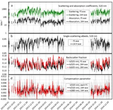
Figure 1.Overview of the data.(a)Scattering and absorption co-efficients atλ=520 nm,(b)single-scattering albedo atλ=520 nm,
(c)backscatter fraction atλ=525 nm andλ=635 nm, and(d)the compensation parameter (k) atλ=520 nm and atλ=880 nm. In
(a–c)the thin lines show the filter-spot-averaged (FS ave) values and in(d)the individual compensation parameters at each filter change (FC). The thick lines show the 24 h-averaged values in all figures.
In the present work the absorption coefficients were calcu-lated according to both the Arnott et al. (2005) and Collaud Coen et al. (2010) algorithms with the respective meanCref values of 4.12 and 4.26 obtained for the Cabauw station by Collaud Coen et al. (2010). The differences of the absorp-tion coefficients calculated from these two algorithms were small and all the conclusions to be presented below were the same. Therefore, even though both algorithms were used, most of the absorption coefficients presented in the figures below were calculated with the formula by Collaud Coen et al. (2010). The average Cref for Cabauw was chosen from Table 4 of Collaud Coen et al. (2010), which presents the
Crefaverages for four stations: Jungfraujoch, Cabauw, Mace Head, and Hohenpeissenberg. Jungfraujoch is a clean, high Alpine site far from emission sources, Hohenpeissenberg a rural mountain site in southern Germany with clean air (e.g., Putaud et al., 2010), and Mace Head a clean marine site on the Irish west coast. Cabauw is in the Netherlands in a re-gion near populated and industrialized areas (e.g., Collaud Coen et al., 2010). Therefore, of these four sites the aerosol in Cabauw can be assumed to be most similar to that ob-served at the SORPES station in Nanjing. A similar value
Cref=4.22 was also obtained by Segura et al. (2014) for a continental station in Spain.
There is a large uncertainty in the Cref even at one sta-tion: for example, in Cabauw the seasonal averages varied
from less than 3 to close to 5 (Collaud Coen et al., 2010), which leads to large uncertainties of bothσapand the single-scattering albedo (ω0=σsp/(σsp+σap)). It is obvious from Eq. (3) that the relative uncertainty ofCrefis also the relative uncertainty ofσap. However, one of the goals of the present work is to study the variations of the compensation param-eter as a function of the variations ofω0so the absoluteω0 values are not that important in this work.
2.4 Averaging
The hypothesis here is that all particles sampled on the filter prior to the spot change affect thekfactor. Therefore all
scat-tering and absorption coefficients, single-scatscat-tering albedos and backscatter fractions were averaged for each aethalome-ter filaethalome-ter spot sampling period. No conventional hourly aver-ages are presented.
Also, the daily or 24 h averages are non-conventional: they were calculated by averaging the compensation param-eters and the corresponding filter-spot-averaged scattering and absorption coefficients that were calculated from the aethalometer filter spot changes during any given day. The number of filter changes to be used for the averaging varied according to the concentration level: during low concentra-tions there may have been only one or two filter spot changes, during high concentrations more. Below, in the analyses of daily averages, only those days have been used during which at least two filter spot changes occurred. During the analyzed period, the average, the median, and the maximum number of filter spot changes were 6.4, 6, and 18 during one day, respectively.
3 Results and discussion 3.1 Overview of the data
Figure 1 shows filterspot-averaged and 24 h-averaged data that fulfilled the criteria for further analyses: the relative hu-midity in the nephelometer sample volume had to be less than 50 %, both the nephelometer and the aethalometer data had to be continuous for at least 24 h. This ruled out summer months (June–August) and most of September. There were 2066 fil-ter spot changes and 342 days that were used for further anal-yses. In the accepted data the average±standard deviation and median of the RH in the nephelometer sample volume were 18±8 % and 16 %, respectively.
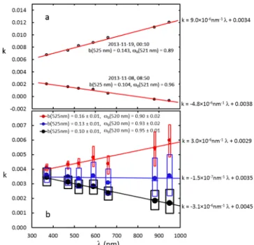
Figure 2.Wavelength dependency of thekfactor(a)on 8 and 19 November 2013 and(b)in the whole data after classification into three bins of the green backscatter fraction. In (b)the box plots present the 25th to 75th percentiles, the middle lines the medians and the circles the averages in each bin. In(a)the lines represent linear regression fittings to the individualkfactors and in(b)linear regression fittings to the averagekin each wavelength and
backscat-ter bin.
There were many several-day-long pollution episodes in November 2013–January 2014 and again the following au-tumn in November 2014 during which scattering and absorp-tion coefficients exceeded 1000 and 100 Mm−1, respectively. The cycling of pollution episodes and cleaner days was also associated with simultaneous cycling ofω0and the backscat-ter fraction b. The slow variations were due to changes in
meteorological conditions and transport routes of air masses. Further analysis of them is out of the scope of the present paper, however.
3.2 Wavelength dependency of the compensation parameter
The compensation parameters (Fig. 1d) calculated for each individual filter-spot change were noisy; for instance, for
λ=520 nm k varied from negative to larger than 0.01 and
at first sight there are only weak common features with the other time series. The noise ofk is due to fast real
tration variations: for instance, if the true BC mass concen-tration is clearly higher just before the filter spot change,k
becomes negative. It was therefore stated already in the orig-inal paper by Virkkula et al. (2007) that during variable con-centrations the use of averagekmay lead to a more
reason-able correction than the individual k values. In the present
work, the daily averaged compensation parameters present
similarities with the time series ofω0 and b: in particular,
when the backscatter fractionbis high, the compensation
pa-rameters seem higher than whenbis low. The compensation
parameter time series (Fig. 1d) also shows that sometimes the greenk(λ=520 nm) was larger than the near-infraredk
(λ=880 nm) and vice versa.
These observations were used and two filter spot changes were picked up during which the filter-spot-averagedbwere
clearly different from each other: on 8 and 19 November 2013 when the backscatter fraction atλ=525 nm was 0.104 and 0.143, respectively (Fig. 2a). Note that during the first filter spot changeω0was clearly higher than during the sec-ond one. Also, the compensation parameters calculated for the seven wavelengths of the aethalometer were very differ-ent for these two spot changes: during the first one they were much lower than during the second one, and during the first one they decreased with wavelength and during the second one they increased with wavelength. Linear regression was applied to this close to linear dependency (Fig. 2a). A line
k=akλ+k0 (4)
was fit through the 7k values obtained for each filter spot
change of the whole data set. Only the slopeak is of inter-est here. Its interpretation is simple: whenak> 0 the com-pensation parameters increase with wavelength, whenak< 0, the compensation parameters decrease with wavelength. As noted already earlier, the compensation parameters obtained for individual spot changes are noisy. Therefore, more rele-vant information was obtained when the compensation pa-rameters from all spot changes were classified according to the associated filter-spot-averaged backscatter fraction of green light and simple descriptive statistics were calculated. Figure 2b shows the averages, medians and the 25th to 75th percentile ranges of the cumulative distributions of the com-pensation parameters at three different backscatter fraction ranges. The lines shown in the figure were fit to the average compensation parameters in each wavelength and bin ofb.
Note again thatω0was high whenbwas low and low when bwas high andakincreased with increasingb.
Another interesting observation can be made about Fig. 2: the range of compensation parameters is larger the longer the wavelength is. This suggests that the longer wavelengths are more sensitive to the factors affecting the compensation. The near-infrared wavelength atλ=880 nm is the one that is used in most aethalometers, even single-wavelength ones, and therefore more attention will be paid to it than to the longest wavelength (λ=950 nm).
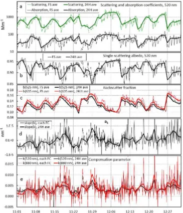
Figure 3. Selected optical properties in November–December 2013. (a) Scattering and absorption coefficients at λ=520 nm,
(b)single-scattering albedo atλ=520 nm,(c)backscatter fraction atλ=525 nm andλ=635 nm,(d)the slope (ak)of the wavelength dependency of the compensation parameter, and(e)the compensa-tion parameter (k) atλ=520 nm and atλ=880 nm. In(a–c)the thin lines show the filter-spot-averaged (FS ave) values, in(d–e)the individual slopes and compensation parameters at each filter change (FC). The thick lines show the 24 h-averaged values in all figures.
Figure 4.The slope of the wavelength dependency of the compen-sation parameter (ak)as a function of the compensation parameter
katλ=880 nm in(a)each filter spot change,(b)24 h averages.
mainly BC, to the aerosol mass in the highly polluted air was clearly lower than during the less-polluted periods, and that the polluted aerosol consisted of some light-scattering ma-terial, for instance of secondary inorganic or organic com-pounds. The other observation is that during the highest pol-lution episodes the backscatter fraction was lower, which suggests that the particles were then bigger than during the less-polluted periods (Fig. 3c). Still another noteworthy
ob-Figure 5.The compensation parameter (k) of individual filter spot
changes calculated for(a)green (λ=520 nm) and(b)near-infrared (λ=880 nm) light as a function of filter-spot-averaged backscatter fraction at the nearest nephelometer wavelengthsλ=525 nm and
λ=635 nm.
servation concerning these four parameters is that there are clear diurnal cycles. To mention one, the diurnal cycle ofω0 is such that the highest values were reached at daytime and the lowest at night, which could be explained so that BC par-ticles get coated during the course of the day by condensation of some scattering material. However, more detailed analy-ses of the pollution episodes and the chemical composition are out of the scope of the present paper.
As far as the compensation parameters (k) and their
wave-length dependency (ak) are concerned, their time series (Fig. 3d and e) reveal features that have similarities with those of the other presented quantities. These are that both
kandak increase and decrease roughly at the same time as band the opposite way compared with ω0. The time series in Fig. 3d and e also show thatak obviously increases and decreases simultaneously withk, which means that they are
not really independent. The scatter plots of both individual and daily averaged ak vs. k at λ=880 nm (Fig. 4) show thatak is linearly dependent on the compensation parame-ter. This means that whenk is known at one wavelength,
it is possible to estimate it at other wavelengths also. The linear fittings in the scatter plots cross the zero line ofak when k(λ=880 nm)=0.0036±0.0022, which means that then all compensation parameters were roughly equal at all wavelengths and whenk(λ=880 nm) was larger than this kincreased with wavelength and vice versa. The above
un-certainty of the zero-line crossing was calculated from the uncertainties of the slope and offset of the linear regressions. 3.3 Effect of backscatter fraction
Since the time series ofkandbhave similarities, it is logical
to calculate their linear regressions. The correlation coeffi-cient of k calculated for each filter change with filter-spot
averaged b is low (Fig. 5). This is due to the high
Table 1.Regression statistics (y=β1x+β0) of compensation parameter vs. backscatter fraction. SE: standard error ofβ1; 95 % confidence
range ofβ1; d.f.: degrees of freedom;t=β1/SE;p:pvalue of the Student’stdistribution.
Calculated by using each filter change
x y r β1 SE 95 % confidence range d.f. t p
b(450) k(470) 0.18 0.024 0.003 (0.018–0.030) 2048 8.2 5.6×10⁻¹⁶ b(525) k(520) 0.22 0.036 0.004 (0.029–0.043) 2048 10.3 2.9×10⁻²⁴ b(635) k(660) 0.21 0.032 0.003 (0.026–0.039) 2048 9.5 5.7×10⁻²¹ b(635) k(880) 0.26 0.056 0.005 (0.047–0.065) 2048 12.4 4.3×10⁻³⁴
Calculated by using all daily averages
x y r β1 SE 95 % confidence range d.f. t p
b(450) k(470) 0.28 0.017 0.003 (0.011–0.024) 320 5.2 3.0×10−07 b(525) k(520) 0.38 0.029 0.004 (0.021–0.037) 320 7.3 2.3×10⁻¹² b(635) k(660) 0.32 0.025 0.004 (0.017–0.033) 320 6. 6.5×10−09 b(635) k(880) 0.43 0.048 0.006 (0.037–0.060) 320 8.4 1.3×10⁻¹⁵
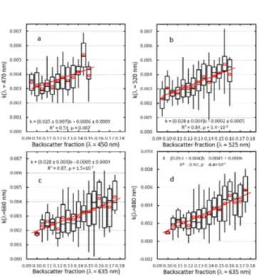
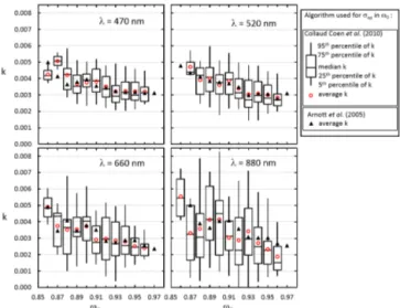
Figure 6. Daily averaged compensation parameters of (a) blue (λ=470 nm), (b) green (λ=520 nm), (c)red (λ=660 nm), and
(d)near-infrared (λ=880 nm) light classified into 0.005 wide bins of the backscatter fraction at the nearest nephelometer wavelengths (λ=450, 525, and 635 nm). The box plots present the 5th, 25th, 50th, 75th, and 95th percentiles and the circles the averages in each bin. The lines are linear fittings to the bin averages and the uncer-tainties of the slope and offset the standard errors obtained from the fitting.
(λ=470, 520, 660, and 880 nm) into bins of backscatter frac-tions at the nearest nephelometer wavelengths (λ=450, 525, and 635 nm) (Fig. 6). The width of the backscatter fraction bins was 0.005. The averages, 5th, 25th, 50th, 75th, and 95th percentiles of the cumulative distribution of the compensa-tion parameters in each bin were calculated.
The compensation parameter medians and averages corre-lated positively with the backscatter fractions, and so did the other percentiles, but their correlation was weaker. Note that the slopes of the linear regressions ofkvs.bare almost the
same when the wavelength of bothkandbare approximately
the same (Fig. 6a–c). Whenkatλ=880 nm is plotted against batλ=635 nm, the slope is almost twice as high.
Instead of paying much attention to the R2 values, it is
more relevant to test the statistical significance of the slope of the regression of compensation parameter vs. backscatter fraction, i.e., β1 in k=β1b+β0. The null hypothesis that the slope is not dependent on the b; i.e.,β1=0 was tested using test statistics given by the estimate of the slope di-vided by its standard error (t=β1/SE). The test statistics
were compared with the Student’s t distribution on n−2 (sample size−number of regression coefficients) degrees of freedom. The regressions were calculated both for each in-dividual filter change and for daily averages. Four compen-sation parameter–backscatter fraction pairs were used: blue:
k(λ=470 nm) vs.b(λ=450 nm), green:k(λ=520 nm) vs. b(λ=525 nm), red k(λ=660 nm) vs. b(λ=635 nm), and red-near-infrared:k(λ=880 nm) vs.b(λ=635 nm). The last combination differs from the other three in that the wave-length ofkandbare not close to the same like in the other
cases. The reason this is considered to be relevant here is that most aethalometers have the 880 nm wavelength and in most three-wavelength nephelometers the longest wave-length is 600–700 nm. The results are presented in Table 1. Thepvalues for all wavelengths are all low (< 0.001), which
gives strong evidence against the null hypothesis, indicating that the slope is not 0 and that there is a linear relationship betweenkandb.
Figure 7.Daily averaged slope (ak)of the compensation parame-ter classified into 0.005 wide bins of the backscatparame-ter fraction of(a) green (λ=525 nm) and(b)red (λ=635 nm) light. The box plots present the 5th, 25th, 50th, 75th, and 95th percentiles and the cir-cles the averages in each bin.
backscatter fraction; see, e.g., the parameterization by An-drews et al. (2006). Müller et al. (2014) showed that for a constant scattering optical depth the optical depth of an aerosol-loaded filter was the higher the smaller thegpof the aerosol was or in other words, the higher the backscatter frac-tion was. This means that when purely scattering aerosol is collected on an aethalometer filter, the optical depth is the larger the larger b is. This should further mean larger
ap-parent absorption coefficients and thus higher BC mass con-centrations with largerb. This is also consistent with
pub-lished measurements made with the new AE 33: Drinovec et al. (2015) reported that the apparent absorption due to small ammonium sulfate particles was clearly larger than that due to large particles. Consequently, the σap and BC should be corrected downwards, i.e., the compensation pa-rameter k should be < 0 and the more negative the larger
the backscatter fraction is. However, for the real atmospheric aerosol the opposite was here observed: the compensation parameter was the larger the larger backscatter fraction was (Fig. 6). This means that the non-corrected absorption coeffi-cients and BC mass concentrations were underestimated the more the higherbwas. Here the qualitative explanation is the
counteracting concept of shadowing, presented by Weingart-ner et al. (2003): due to enhanced scattering the absorbing particles absorb a higher fraction of light and effectively re-duce the optical path. This leads to an underestimation of the true σap and BC and therefore the compensation parameter should be positive.
Also,ak, the wavelength dependency of the compensation parameter depends on the backscatter fraction. Especially the relationship betweenakandbof green light is strikingly lin-ear (Fig. 7). At b (λ=525 nm)≈0.13, ak≈0, for smaller backscatter fractions ak< 0 and for larger backscatter frac-tions ak> 0. No detailed explanation can be given at this point but qualitatively the above relationship means that for small particles the correction is the larger the larger the wave-length is and for large particles the other way around.
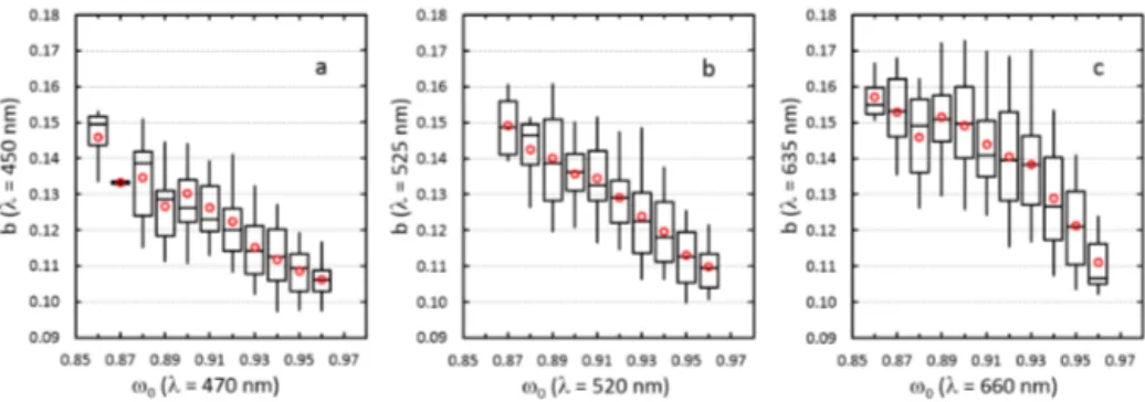
Figure 8. Daily averaged compensation parameters of blue (λ=470 nm), green (λ=520 nm), red (λ=660 nm), and near-infrared (λ=880 nm) light classified into 0.01 wide bins of the single-scattering albedo (ω0) at the same wavelengths. The box
plots present the 5th, 25th, 50th, 75th, and 95th percentiles and the circles the averages in each bin. Mostω0bins are based onσap cal-culated with the Collaud Coen et al. (2010) algorithm; the black tri-angles are the averages of compensation parameters classified into
ω0 bins with theσap calculated by using the Arnott et al. (2005) algorithm.
3.4 Effect of single-scattering albedo
The relationship of the single-scattering albedo and the com-pensation parameter was analyzed analogically. Theks were
classified into bins ofω0at four aethalometer wavelengths (λ=470, 520, 660, and 880 nm). The width of theω0bins was 0.01. The averages, 5th, 25th, 50th, 75th, and 95th per-centiles of the cumulative distribution of the compensation parameters were calculated. The bin averages and medians decreased almost monotonically with increasingω0, but the ranges were large (Fig. 8). Note that in Fig. 8 the k vs. ω0 relationship of the bin averages is plotted both by using the Collaud Coen et al. (2010) algorithm and the Arnott et al. (2005) algorithm simply to show that the main relation-ship, decreasingkwith increasingω0, did not depend on the algorithm used for calculating absorption coefficients σap. It is worth noting at this point that the absolute values of
σapandω0are very uncertain because of the uncertainty of the multiple scattering correction factorCref. Theω0values shown in Fig. 8 were calculated withCrefvalues of 4.12 and 4.26 as explained above but ifCrefis smallerω0is lower than that shown in Fig. 8. This would not change the main result:
Table 2. Regression statistics (y=β1x+β0) of compensation parameter vs. single-scattering albedo. Detailed column description as in
Table 1.
Calculated by using each filter change
x y r β1 SE 95 % confidence range d.f. t p
ω0(470) k(470) 0.07 −0.006 0.002 (−0.009–−0.002) 2048 −3.4 7.3×10−04 ω0(520) k(520) 0.08 −0.008 0.002 (−0.012–−0.004) 2048 −3.8 1.3×10−04 ω0(660) k(660) 0.07 −0.007 0.002 (−0.012–−0.003) 2048 −3.1 2.0×10−03 ω0(880) k(880) 0.08 −0.010 0.003 (−0.016–−0.004) 2048 −3.5 4.7×10−04
Calculated by using all daily averages
x y r β1 SE 95 % confidence range d.f. t p
ω0(470) k(470) 0.27 −0.011 0.002 (−0.016–−0.007) 320 −5.1 5.9×10−07 ω0(520) k(520) 0.31 −0.015 0.003 (−0.020–−0.010) 320 −5.9 9.6×10−09 ω0(660) k(660) 0.26 −0.015 0.003 (−0.021–−0.009) 320 −4.8 2.0×10−06 ω0(880) k(880) 0.25 −0.019 0.004 (−0.027–−0.011) 320 −4.5 8.1×10−06
Figure 9.Daily averaged slope (ak)of the compensation parameter
classified into 0.01 wide bins of the single-scattering albedo (ω0)at
(a)green (λ=520 nm) and(b)red (λ=660 nm) wavelengths. The box plots present the 5th, 25th, 50th, 75th, and 95th percentiles and the circles the averages in each bin.
enough to conclude that the relationship is statistically sig-nificant.
A simple theoretical explanation for the decreasingkwith
increasingω0can be given. If it is assumed that (1) the load-ing correction function f in Eq. (3) equals 1+kATN and
(2) that the dependence on the scattering coefficient is incor-porated into the compensation parameter, the equation for the absorption coefficient becomes
σap=
1+kATN
Cref σ0. (5)
On the other hand, if it is assumed that the absorption coef-ficient is calculated from Eq. (3) where f is not the same
function as in Eq. (5) and where the dependence on the scattering coefficient is explicitly presented and if the two Eqs. (3) and (5) are set equal the compensation parameter
can be solved as 1+kATN
Cref σ0
=f σ0−sσsp Cref
⇔k= 1
ATN
f−1−sσsp σ0
. (6)
When Eq. (3) is again rearranged as σ0=(Crefσap+ sσsp)/f and inserted in Eq. (6), the compensation parame-ter can be expressed as
k= 1
ATN
f−1− sσsp Crefσap+sσsp
f
= 1
ATN f 1−
σsp Cref
s σap+σsp !
−1 !
. (7)
The term σsp/ C
ref
s σap+σsp
is not exactly identical to the single-scattering albedoω0, but it also approaches unity whenω0approaches unity andf (1−σsp/(Csrefσap+σsp))→ 0, and thenkmay even become negative. In other words, the
compensation parameter can be negative but the resulting ab-sorption coefficient can never be negative; this sets the limit to it.
The relationship between ak and the single-scattering albedo is very similar to that betweenkandω0: also,ak de-creases with increasingω0(Fig. 9). In other words for darker aerosols,ω0less than approximately 0.92, the correction in-creases with wavelength and at higherω0it decreases with wavelength. No theoretical explanation could be given at this point.
3.5 Separating the effects of single-scattering albedo and backscatter fraction
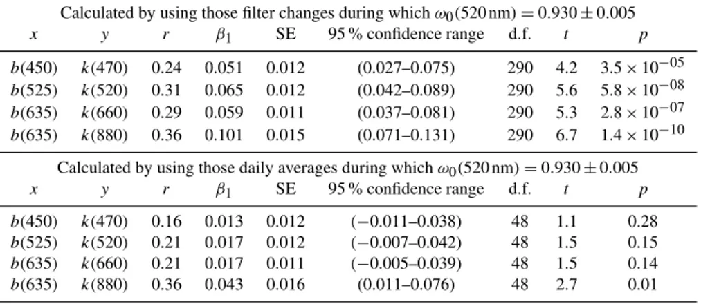
Figure 10.Daily averaged backscatter fraction (b)of(a)blue,(b)green and(c)red light classified into 0.01 wide bins of the single-scattering albedo (ω0). Note:bis that measured at the nephelometer wavelengths 450, 525 and 635 nm andω0is that at the aethalometer wavelengths
470, 520 and 660 nm. The box plots present the 5th, 25th, 50th, 75th, and 95th percentiles and the circles the averages in each bin.
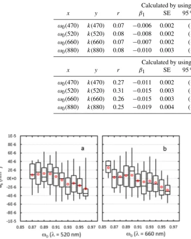
Figure 11. Compensation parameters at the aethalometer green wavelength (λ=520 nm) as a function of(a)the backscatter frac-tionband(b)the single-scattering albedoω0whenbandω0were
in a narrow range:(a)contains data from those filter changes during which the filter-spot-averaged ω0(λ=520 nm)=0.930±0.005.
(b)contains data from those filter changes during which the filter-spot-averaged b(λ=525 nm)=0.130±0.005. The red lines and the equations represent linear regressions fitted to the data.
data available here sinceω0andbwere not really
indepen-dent. The darkest aerosol, i.e., the aerosol with the lowest
ω0, was observed when the backscatter fraction was the high-est (Fig. 10), sugghigh-esting that the particle size of the darkhigh-est aerosol was also the smallest.
To disconnect the two effects the data were further classified into (a) a narrow ω0 range ω0(λ=520 nm)=0.930±0.005 for which linear re-gressions of k vs. b were calculated and (b) a narrow b
range (b(λ=525 nm)=0.130±0.005) for which linear regressions of k vs. ω0 were calculated. The regressions
within these ranges were calculated both for each filter-spot change and for the daily averaged data as above. The linear regressions of the compensation parameters at λ=520 nm for the individual spot changes are pre presented in Fig. 11 and for the rest of the linear regressions in Tables 3 and 4.
In the individual filter-change regressions there was now a clearly more significant dependence ofk onb (p< 10−4)
than on ω0 (p=0.01–0.1). For the k vs. ω0 the slope es-timates β1were actually positive (Table 4), meaning thatk
would increase with increasingω0, which is just the opposite
observation of that made from all the data. The 95 % confi-dence ranges, on the other hand, include both negative and positive slopes and thepvalues are high. An exception is the kvs.ω0atλ=880 nm: the confidence range is positive and the p value low. Based on the regression of this one wave-length only it is better not to draw any strong conclusions, however. For the daily averages thepvalues of most
regres-sions were > 0.1 and the 95 % ranges had both negative and positive values (Tables 3 and 4), showing that in the daily averaged classified data there was no evidence for the linear relationships ofkvs.bandkvs.ω0. There was one exception however, this timekatλ=880 nm vs.batλ=635 nm with p=0.01 and the 95 % range ofβ1> 0.
The above exercise was done to find which one, the single-scattering albedo or the backscatter fraction affects the com-pensation parameter more. The p values of the individual
filter-spot regressions suggest that the effect of the backscat-ter fraction is more dominant than that ofω0. But since the regressions of the daily averaged data do not show this, it should not be considered proven. To study it in a laboratory, one should produce aerosols that have the same size (andb)
but variableω0. This is difficult because if variations inω0 are accomplished by coating pure BC by condensing some scattering material, the particles grow andbdecreases.
3.6 Possible implementation into a data analysis algorithm
If the relationships betweenk,ω0, andbwere unambiguous
aethalometer data could in principle be used in an algorithm for estimating ω0 andb. However, as it was shown in the
previous section, even after the classifications intoω0andb
bins there was still a large range of compensation parame-ters that remained unexplained. A probable reason may have been rapidly varying BC mass concentrations, as mentioned several times above, but there are also other possible expla-nations.
Table 3.Regression statistics (y=β1x+β0)of compensation parameter vs. backscatter fraction at a limited single-scattering albedo range.
Detailed column description as in Table 1.
Calculated by using those filter changes during whichω0(520 nm)=0.930±0.005 x y r β1 SE 95 % confidence range d.f. t p
b(450) k(470) 0.24 0.051 0.012 (0.027–0.075) 290 4.2 3.5×10−05 b(525) k(520) 0.31 0.065 0.012 (0.042–0.089) 290 5.6 5.8×10−08 b(635) k(660) 0.29 0.059 0.011 (0.037–0.081) 290 5.3 2.8×10−07 b(635) k(880) 0.36 0.101 0.015 (0.071–0.131) 290 6.7 1.4×10⁻¹⁰
Calculated by using those daily averages during whichω0(520 nm)=0.930±0.005 x y r β1 SE 95 % confidence range d.f. t p
b(450) k(470) 0.16 0.013 0.012 (−0.011–0.038) 48 1.1 0.28 b(525) k(520) 0.21 0.017 0.012 (−0.007–0.042) 48 1.5 0.15 b(635) k(660) 0.21 0.017 0.011 (−0.005–0.039) 48 1.5 0.14 b(635) k(880) 0.36 0.043 0.016 (0.011–0.076) 48 2.7 0.01
Table 4.Regression statistics (y=β1x+β0) of compensation parameter vs. single-scattering albedo at a limited backscatter fraction range. Detailed column description as in Table 1.
Calculated by using those filter changes during whichb(525 nm)=0.130±0.005 x y r β1 SE 95 % confidence range d.f. t p
ω0(470) k(470) 0.08 0.009 0.006 (−0.002–0.021) 411 1.7 0.10 ω0(520) k(520) 0.08 0.011 0.006 (−0.002–0.023) 411 1.6 0.10 ω0(660) k(660) 0.09 0.014 0.008 (−0.001–0.029) 411 1.9 0.06 ω0(880) k(880) 0.13 0.024 0.009 (0.006–0.043) 411 2.6 0.01
Calculated by using those daily averages during whichb(525 nm)=0.130±0.005 x y r β1 SE 95 % confidence range d.f. t p
ω0(470) k(470) 0.04 −0.002 0.008 (−0.018–0.013) 66 −0.3 0.77 ω0(520) k(520) 0.03 −0.002 0.009 (−0.020–0.015) 66 −0.2 0.80 ω0(660) k(660) 0.05 0.004 0.010 (−0.015–0.024) 66 0.4 0.68 ω0(880) k(880) 0.18 0.017 0.012 (−0.006–0.041) 66 1.5 0.14
was no method available to measure it. It is likely that the same amount of absorbing aerosol such as BC yields differ-ent compensation parameters when it is internally mixed with scattering material and when these two are externally mixed. In these cases the penetration depths of BC particles into the filter would be different even if the overall backscatter frac-tion of the aerosol were the same. Therefore it is not likely there will be an unambiguous relationship betweenk,ω0, and b. However, for internally mixed, typical aged BC aerosol,
future research may prove out that the relationship is simple enough to be implemented into an algorithm.
4 Summary and conclusions
Aerosol optical properties were measured with a seven-wavelength aethalometer and a three-seven-wavelength neph-elometer at the suburban site SORPES in Nanjing, China, in September 2013–January 2015. The most important re-sult obtained from the analysis of the data is that quan-tities calculated from two independent methods; i.e., the backscatter fraction measured with the nephelometer and the compensation parameter k, calculated from the
aethalome-ter data with the Virkkula et al. (2007) algorithm, were
correlated. Atλ=660 nm the daily averaged compensation parameter k≈0.0017±0.0002 and 0.0042±0.0013 when the backscatter fraction at λ=635 nm was in the ranges of 0.100±0.005 and 0.160±0.005, respectively. Also, the wavelength dependency of the compensation parameter de-pended on the backscatter fraction: whenb(λ=525 nm) was less than approximately 0.13 the compensation parameter de-creased with wavelength and at largerb it increased with
wavelength. This dependency has not been considered in any of the algorithms that are currently used for process-ing aethalometer data. The compensation parameter also de-pended on the single-scattering albedo ω0 so that k
de-creased with increasingω0. For the green light (λ=520 nm) in theω0range 0.870±0.005, the average (±standard devi-ation)k≈0.0047±0.006 and in theω0range 0.960±0.005, k≈0.0028±0.0007. This difference was larger for the near-infrared light (λ=880 nm): in the ω0 range 860±0.005, k≈0.0055±0.0023 and in the ω0 range 0.960±0.005, k≈0.0019±0.0011. The negative dependence on ω0 was also shown with a simple theoretical analysis.
the lowest single-scattering albedo had the highest backscat-ter fractions. An attempt was made to separate the effects of these two parameters. The selection of one narrowω0bin and classifying the compensation parameters again as a function ofband the selection of a narrow backscatter fraction bin and
classifying the compensation parameters again as a function of ω0suggests thatb may be even more important a factor
than ω0. However, even after classifying the compensation parameters intoω0andbbins there was still a large range of
compensation parameters that remained unexplained. In ad-dition to rapidly varying concentrations a possible explana-tory factor is the mixing state of the aerosols that was not measured.
In spite of the uncertainties, the most important conclusion is that the backscatter fraction of the aerosol has a very clear effect on the aethalometer data and it should be taken into account. To quantify this in terms ofσapor BC mass concen-trations, assume that b=0.16 and that ATN=80, a typical value for the red wavelength prior to filter spot change. The above averagekfor the red wavelength yield for the whole
compensation function f =1+kATN≈1.34. This means that without the compensation the BC mass concentration or the absorption coefficient may be even tens of percent too low.
The underlying reasons for the effect of the backscatter fraction are the variations in the enhanced scattering due to variations in the asymmetry parameter and variations in the penetration depth of the particles into the filter, which de-pend on their size. This observation is important especially in China where anthropogenic pollution is often mixed with desert dust: the backscatter fraction is large for small parti-cles and small for large partiparti-cles such as soil dust.
Another, related conclusion is that also the multiple-scattering correction factorCrefmay potentially be a function of bothbandω0. Collaud Coen et al. (2010) found thatCref decreased with increasing ω0. But they also found thatCref varied considerably even at one measurement site and hy-pothesized that it might be due to semi-volatile organic com-pounds and water vapor condensing on the filter fibers or to other similar phenomena. In the present study, neither a new
Crefnor any algorithm for getting the absorption coefficient was even attempted to be derived due to a lacking indepen-dent absorption method. In the future this should be done by using for instance an extinction instrument or a photoacous-tic spectrometer together with the aethalometer and the neph-elometer. Ideally, the measurement setup would also contain a method for measuring the mixing state of the aerosol, for instance an SP2 instrument or a Volatility Tandem Differen-tial Mobility Analyzer (VTDMA). If it turns out thatCrefalso depends on the backscatter fraction and the single-scattering albedo in a predictable way, then the relationships betweenk, b, andω0could in principle also be used for estimatingCref. This study was conducted by analyzing data collected with the AE31 aethalometer model, which uses a different filter material and the flow setup than the new AE33 aethalometer
model. Also, the compensation factor is calculated there in a slightly different way, but it was shown above that in princi-ple the difference is not big. Therefore the results presented above will most probably not be quantitatively the same, but it is very likely that the qualitative results are the same: the larger the backscatter fraction is, the larger are the compensa-tion parameter and the slope of the wavelength dependency on it, and the other way around when comparing with the single-scattering albedo. This can be considered as a recom-mendation for future research.
Data availability
To obtain the data used in the paper, please contact the cor-responding author.
Acknowledgements. The research was supported by the Jiangsu
Provincial Natural Science Fund (no. BK20140021), National Science Foundation of China (D0510/41275129), and Academy of Finland’s Centre of Excellence program (Centre of Excellence in Atmospheric Science – From Molecular and Biological processes to The Global Climate, project no. 272041).
Edited by: W. Maenhaut
References
Andrews, E., Sheridan, P. J., Fiebig, M., McComiskey, A., Ogren, J. A., Arnott, P., Covert, D., Elleman, R., Gasparini, R., Collins, D., Jonsson, H., Schmid, B., and Wang, J.: Comparison of methods for deriving aerosol asymmetry parameter, J. Geo-phys. Res.-Atmos., 111, D05S04, doi:10.1029/2004JD005734, 2006.
Arnott, W. P., Hamasha, K., Moosmuller, H., Sheridan, P. J., and Ogren, J. A.: Towards aerosol light-absorption measurements with a 7-wavelength aethalometer: evaluation with a photoa-coustic instrument and 3-wavelength nephelometer, Aerosol Sci. Tech., 39, 17–29, doi:10.1080/027868290901972, 2005. Cheng, Y.-H. and Yang, L.-S.: Correcting aethalometer black
car-bon data for measurement artifacts by using inter-comparison methodology based on two different light attenuation in-creasing rates, Atmos. Meas. Tech. Discuss., 8, 2851–2879, doi:10.5194/amtd-8-2851-2015, 2015.
Collaud Coen, M., Weingartner, E., Apituley, A., Ceburnis, D., Fierz-Schmidhauser, R., Flentje, H., Henzing, J. S., Jen-nings, S. G., Moerman, M., Petzold, A., Schmid, O., and Bal-tensperger, U.: Minimizing light absorption measurement arti-facts of the Aethalometer: evaluation of five correction algo-rithms, Atmos. Meas. Tech., 3, 457–474, doi:10.5194/amt-3-457-2010, 2010.
Ding, A. J., Fu, C. B., Yang, X. Q., Sun, J. N., Petäjä, T., Ker-minen, V.-M., Wang, T., Xie, Y., Herrmann, E., Zheng, L. F., Nie, W., Liu, Q., Wei, X. L., and Kulmala, M.: Intense atmo-spheric pollution modifies weather: a case of mixed biomass burning with fossil fuel combustion pollution in eastern China, Atmos. Chem. Phys., 13, 10545–10554, doi:10.5194/acp-13-10545-2013, 2013b.
Drinovec, L., Moˇcnik, G., Zotter, P., Prévôt, A. S. H., Ruck-stuhl, C., Coz, E., Rupakheti, M., Sciare, J., Müller, T., Wieden-sohler, A., and Hansen, A. D. A.: The “dual-spot” Aethalome-ter: an improved measurement of aerosol black carbon with real-time loading compensation, Atmos. Meas. Tech., 8, 1965–1979, doi:10.5194/amt-8-1965-2015, 2015.
Heal, M. R. and Hammonds, M. D.: Insights into the composition and sources of rural, urban and roadside carbonaceous PM10, Environ. Sci. Technol., 48, 8995–9003, 2014
IPCC: Climate Change 2013: the Physical Science Basis, con-tribution of Working Group I to the Fifth Assessment Report of the Intergovernmental Panel on Climate Change, edited by: Stocker, T. F., Qin, D., Plattner, G.-K., Tignor, M., Allen, S. K., Boschung, J., Nauels, A., Xia, Y., Bex, V., and Midgley, P. M.: Cambridge University Press, Cambridge, UK and New York, NY, USA, 1535 pp., 2013.
Lack, D. A., Cappa, C. D., Cross, E. S., Massoli, P., Ahern, A. T., Davidovits, P., and Onasch, T. B.: Absorption enhancement of coated absorbing aerosols: validation of the photo-acoustic tech-nique for measuring the enhancement, Aerosol Sci. Tech., 43, 1006–1012, doi:10.1080/02786820903117932, 2009.
Moteki, N., Kondo, Y., Nakayama, T., Kita, K., Sahu, L., Ishi-gai, T., Kinase, T., and Matsumi, Y.: Radiative transfer modeling of filter-based measurements of light absorption by particles: im-portance of particle size dependent penetration depth, J. Aerosol Sci., 41, 401–412, doi:10.1016/j.jaerosci.2010.01.004, 2010. Müller, T., Laborde, M., Kassell, G., and Wiedensohler, A.: Design
and performance of a three-wavelength LED-based total scatter and backscatter integrating nephelometer, Atmos. Meas. Tech., 4, 1291–1303, doi:10.5194/amt-4-1291-2011, 2011.
Müller, T., Virkkula, A., and Ogren, J. A.: Constrained two-stream algorithm for calculating aerosol light absorption coefficient from the Particle Soot Absorption Photometer, Atmos. Meas. Tech., 7, 4049–4070, doi:10.5194/amt-7-4049-2014, 2014. Nakayama, T., Kondo, Y., Moteki, N., Sahu, L. K., Kinase, T.,
Kita, K., and Matsumi, Y.: Size-dependent correction factors for absorption measurements using filter-based photometers: PSAP and COSMOS, J. Aerosol Sci., 41, 333–343, 2010.
Park, S. S., Hansen, A. D. A., and Cho, Y.: Measurement of real time black carbon for investigating spot loading ef-fects of Aethalometer data, Atmos. Environ., 11, 1449–1455, doi:10.1016/j.atmosenv.2010.01.025, 2010.
Putaud, J.-P., Dingenen, R. V., Alastuey, A., et al.: A European aerosol phenomenology – 3: physical and chemical charac-teristics of particulate matter from 60 rural, urban, and kerb-side sites across Europe, Atmos. Environ., 44, 1308–1320, doi:10.1016/j.atmosenv.2009.12.011, 2010.
Schmid, O., Artaxo, P., Arnott, W. P., Chand, D., Gatti, L. V., Frank, G. P., Hoffer, A., Schnaiter, M., and Andreae, M. O.: Spectral light absorption by ambient aerosols influenced by biomass burning in the Amazon Basin. I: Comparison and field calibration of absorption measurement techniques, At-mos. Chem. Phys., 6, 3443–3462, doi:10.5194/acp-6-3443-2006, 2006.
Segura, S., Estellés, V., Titos, G., Lyamani, H., Utrillas, M. P., Zot-ter, P., Prévôt, A. S. H., Moˇcnik, G., Alados-Arboledas, L., and Martínez-Lozano, J. A.: Determination and analysis of in situ spectral aerosol optical properties by a multi-instrumental ap-proach, Atmos. Meas. Tech., 7, 2373–2387, doi:10.5194/amt-7-2373-2014, 2014.
Shen, Y., Chi, X., Ding, A., Nie, W., Qi, Zheng, L., Huang, X., Xie, Y., Wang, J., Virkkula, A., Petäjä, T., and Kulmala, M.: Sea-sonal and diurnal cycles of in situ aerosol optical properties at the SORPES station in Nanjing, China, Atmos. Chem. Phys., in preparation, 2015.
Song, S., Wu, Y., Xu, J., Ohara, T, Hasegawa, S., Li, J., Yang, L., and Hao, J.: Black carbon at a roadside site in Beijing: temporal variations and relationships with carbon monoxide and particle number size distribution, Atmos. Environ., 77, 213–221, 2013. Virkkula, A., Mäkelä, T., Yli-Tuomi, T., Hirsikko, A.,
Kopo-nen, I. K., Hämeri, K., and Hillamo, R.: A simple procedure for correcting loading effects of aethalometer data, J. Air Waste Manage., 57, 1214–1222, doi:10.3155/1047-3289.57.10.1214, 2007.
Wang, Y., Hopke, P. K., Rattigan, O. V., Xia, X., Chalupa, D. C., and Utell, M. J.: Characterization of residential wood combustion particles using the two-wavelength aethalometer, Environ. Sci. Technol., 45, 7387–7393, 2011.
Weingartner, E., Saathoff, H., Schnaiter, M., Streit, N., Bitnar, B., and Baltensperger, U.: Absorption of light by soot particles: de-termination of the absorption coefficient by means of aethalome-ters, J. Aerosol Sci., 34, 1445–1463, 2003.