Application of Receptor Models on Water Quality Data in Source Apportionment in Kuantan River Basin

R E S E A R C H A R T I C L E

Open Access

Application of receptor models on water quality

data in source apportionment in Kuantan River

Basin

Mohd Fahmi Mohd Nasir

, Munirah Abdul Zali

, Hafizan Juahir

, Hashimah Hussain

, Sharifuddin M Zain

and Norlafifah Ramli

Abstract

Recent techniques in the management of surface river water have been expanding the demand on the method that can provide more representative of multivariate data set. A proper technique of the architecture of artificial neural network (ANN) model and multiple linear regression (MLR) provides an advance tool for surface water modeling and forecasting. The development of receptor model was applied in order to determine the major sources of pollutants at Kuantan River Basin, Malaysia. Thirteen water quality parameters were used in principal component analysis (PCA) and new variables of fertilizer waste, surface runoff, anthropogenic input, chemical and mineral changes and erosion are successfully developed for modeling purposes. Two models were compared in terms of efficiency and goodness-of-fit for water quality index (WQI) prediction. The results show that APCS-ANN model gives better performance with highR2value (0.9680) and small root mean square error (RMSE) value (2.6409) compared to APCS-MLR model. Meanwhile from the sensitivity analysis, fertilizer waste acts as the dominant pollutant contributor (59.82%) to the basin studied followed by anthropogenic input (22.48%), surface runoff (13.42%), erosion (2.33%) and lastly chemical and mineral changes (1.95%). Thus, this study concluded that receptor modeling of APCS-ANN can be used to solve various constraints in environmental problem that exist between water distribution variables toward appropriate water quality management.

Keywords:Water quality, Receptor modeling, Multiple linear regression (MLR), Artificial neural network (ANN)

Introduction

Surface water quality studies are among the preliminary topics in Malaysia which provide an overview on the sta-tus of the specified river. In addition, surface waters are most susceptible due to easy accessibility for wastewater (Singh et al., [1]) and anthropogenic activities from its vicinity. Although 60% of the main rivers in Malaysia are regulated for domestic, agricultural and industrial fields (DID, [2]); sewage disposal, industrial effluents (Rosnani, [3]) and urbanization are among the major pollution sources influencing the health of the rivers in Malaysia (Figure 1). Monitoring and the study of surface water will then offer judgments on the authorities to the offen-der and the concerns of researchers in the field of

ecotoxicology and risk assessment if other contaminants such as inorganic and organic micropollutants that may affect water quality.

Monitoring programs often worked out with frequent water samplings at many sampling sites all over the world and determination of physiochemical parameters can provide a representative and dependable estimation of the surface water quality. In Malaysia, Department of Environment (DOE) has been conducting unstoppable monitoring activities since 1978 resulting to large data matrix collection and desperately requires remarkable statistical tools such as multivariate and artificial intelli-gent for exceptional data illustration.

The program covered initially all the river basin in Malaysia, involving mainly manual sampling andin-situ measurements of the river water quality. According to the DOE’s Environmental Quality Report in 2007, 158 river basins are involved in this program to monitor

* Correspondence:hafizan@env.upm.edu.my

1_{Department of Environmental Sciences, Faculty of Environmental Studies,}

UPM Serdang, Selangor, Malaysia

Full list of author information is available at the end of the article

river quality changes on a continuous basis (DOE, [4]). Even though DOE have a regular monitoring program to provide the complex environmental data sets, however they are is still lacking in the application of multivariate statistical methods. This is in attempt to extract all pos-sible information from the river water quality data sets and consequently determine the major sources that in-fluencing the river class at Kuantan River Basin. The multivariate statistical technique and exploratory data analysis are the appropriate tools for a meaningful data reduction and interpretation of multi-constituent chem-ical and physchem-ical measurement (Massartet al., [5]).

Water quality is referring to the characteristics of water whether in its physical, chemical or biological character. Based on the water quality data, the water quality index (WQI) was developed to evaluate the water quality status and river classification in Malaysia. WQI provides a useful way to predict changes and trends in the water quality by considering multiple parameters. WQI is formed by six selected water quality variables, namely dissolved oxygen (DO), BOD, chemical oxygen demand (COD), SS, AN and pH (DOE, [6]). WQI values are in the range 0_–100. If the values are in the range of 81_–100 the samples water analyzed in the specific sta-tion fall in clean category. Values ranging from 60_–80 and 0_–59 are grouped as slightly polluted and polluted area respectively.

Continuous monitoring of river water quality reveals the chemical and physico-chemical parameters for the in-terpretation of large data set with many variables; there-fore environmetric approach need to be constructed to comprehend the variation on the data since it is not en-tirely convincing. In this study, the large data matrix obtained from monitoring programme conducted by DOE, Malaysia from year 2003 to 2007 was introduced to

receptor models techniques that involved varimax factor from principal components analysis (PCA) with two dif-ferent data based on multiple linear regression (MLR) and artificial neural network (ANN) models. These approaches were conducted in many fields such as pre-diction of ozone concentrations (Bandyopadhyay and Chattopadhyay, [7]; Sousaet al., [8]), forecasting summer-time (Chaloulakou et al., [9]), prediction medical waste generation (Jahandideh et al., [10]), prediction the lower heating value of municipal solid waste (Ogwueleka and Ogwueleka, [11]) however emphasis in water quality were not yet steady especially in tropical regions. The develop-ment of such mathematical tools will facilitate an early warning for people whom reside near the river other than to environmental agencies in order to protect and con-serve the river from further being soiled by pollutions.

Source apportionment techniques were applied in the data set by combining PCA with MLR and PCA with ANN. The aim of this study is to discover the major pol-lution sources that significantly change the WQI values in Kuantan River Basin from the varimax factors pro-duced for MLR and ANN models. The uncorrelated new variables that account much of the original data will be used as input variables for the models; other than com-bining statistical and an artificial intelligent techniques which has been received great spotlight in environmen-tal pattern recognition study (Sousaet al., [8]). Moreover the particular discussions on comparison for both tech-niques were not extensively reported in water quality study. Thus, this study will determine the models that best fit on the entire data sets by performing non-linear transformation of input data (resulted VFs) to approxi-mate WQI values.

works. However its application in water quality study were less published and lead to this study aimed to certify whether this model were applicable for WQI forecasting in Kuantan River Basin. Despite the fact that many studies performed concluded that there is no general best model-ling techniques, it still depends on the scope and objec-tives of the studies (Aertsenet al., [19]).

The objectives of this study are to predict WQI values as well as to estimate the main contributor using MLR and ANN model from the varimax factors generated by PCA. This study will provide comprehensive under-standing on goodness and weakness for both models and consequently finalised the correct model for WQI prediction in the Kuantan River Basin.

Materials and methods Study area

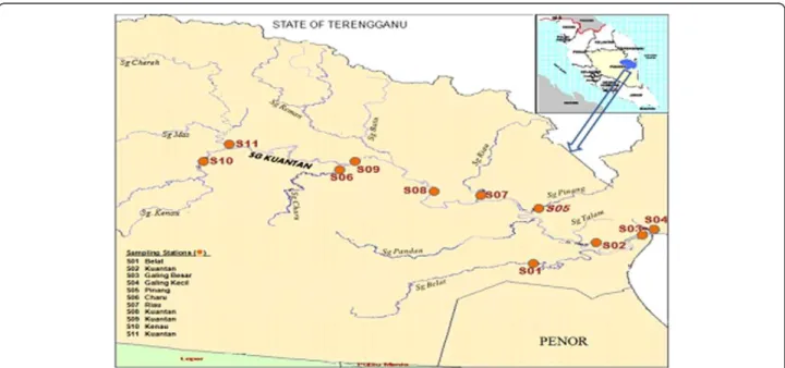
Kuantan River Basin is in the district of Kuantan at the north eastern end of Pahang State in Peninsular Malaysia (Figure 2). It is one of the important river basins in Pahang and covers an area of 1630 km2 cat-chment area which started from forest reserved area in Mukim Ulu Kuantan through agricultural areas, Kuantan town (state capital of Pahang) towards the South China Sea. Kuantan River Basin consists of several important tributaries and these rivers drain the major rural, agricultural, urban and industrial areas of Kuantan District and discharge into South China Sea.

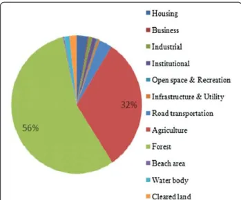
Kuantan River basin which is in Kuantan District area has six administrative mukims (small district). In terms of land use, the main types of land use in this district are forest and agriculture that cover approximately 56% and

32% respectively, from the whole area of Kuantan Dis-trict. Majority of the forested areas are at the west of Kuantan District or in upstream of the basin. Besides that, there is an ex-tin mining land in Sungai Lembing or at upstream or low sub basin area. The mining activ-ities was started in 1906 and stopped in 1986 due to eco-nomic recession in our country.

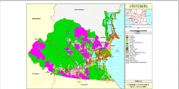
In term of land use utilisation, agriculture is considered to be one of the main economic activities in this river basin where it covers about 70,128 hectares of the area (DOE, [20]). According to land use map of Kuantan Dis-trict as shown in Figure 3, main agricultural area is located in the middle part of the basin. The oil palm is the main agricultural crops (57,863 hectares), followed by rubber (10,191 hectares). Fruits are the third largest agricultural crops which covers the total area of 1,489 hectares.

There are three palm oil mills which are the major agro-based industries in the middle of the basin and might be contributed to deterioration of Kuantan river water quality (DOE, [21]). Recently, 42 tributaries in Peninsular Malaysia have been categorized as very pol-luted (Aiken et al., [22]). Since 1999, there were 13 pol-luted tributaries all over Malaysia with 36 polpol-luted rivers due to human activities such as industry, construction and agriculture (DOE, [20]).

Data and parameters

The water quality data were collected in 2003 to 2007 from eleven monitoring stations provided by DOE. How-ever, some of the stations are inconsistently sampling thus leading to the missing data. Thirty water quality parameters are selected by DOE in order to represent the

water quality in the river. Unfortunately only 13 para-meters are consistently sampled along 2003 to 2007 there-fore a total of 275 observations were used for source apportionment and modeling techniques. The thirteen water quality parameters are selected for analysis in this study are: pH, dissolve oxygen (DO), biological oxygen de-mand (BOD), chemical oxygen dede-mand (COD), suspended solid (SS), ammoniacal nitrogen (AN), dissolved solids (DS), total solids (TS), nitrate (NO3), chloride (Cl-), phos-phate (PO4

-), Escherichia coli (E. coli) and coliform. According to DOE [6], the water quality index (WQI) was developed to evaluate the water quality status and river classification. WQI consists of six selected water quality parameters known as DO, BOD, COD, SS, AN, and pH which provides useful way to predict the changes and trends in the water quality (DOE, [6]).

Data preprocessing

The data were initially arranged according to the sta-tions and year of monitoring. Variables that are not have been detected (below detection limit) were set to half of its detection limit in order to ensure that there is no missing data in the dataset. Normality test were per-formed using the Anderson-Darling test since the multi-variate statistical techniques requires the variables to be normally distributed (Zhou et al., [23]). Data that are not normally distributed undergo pretreatment which consist of centering, standardization and log-scaling method. Standardization opts to increase the influence of variables with small variance and vice versa (Krishna et al., [24]). Log scaling was used upon variables which

exhibit too low or high values (Felipe-Soteloet al., [25]). Statistical computation of PCA and MLR were carried out using XLSTAT 2010 Excel add-in Window software and prediction model of ANN was conducted by using JMP8 for Windows software (Camdevyrenet al., [26]).

Principal component analysis (PCA)

The most powerful technique for pattern recognition that attempts to explain the variance of a large set of inter-correlated variables and transforming it into smaller set of independent (uncorrelated) variables (principal compo-nents). PCA aims to uncover a more underlying set of fac-tors that accounts for the major pattern across all the original variables (Saim et al., [27]). Moreover PC also, present information on the most meaningful parameters, which define whole data, set affording data reduction with minimum loss of original information (Krishna et al., [24]). This technique provides information on the most significant parameters by rendering data reduction with minimum loss of original information (Vega et al., [28]; Helenaet al., [29]; Wunderlinet al., [30]). PCA is sensitive to outliers, missing data, and poor linear correlation be-tween variables due to inadequate assigned variables (Sarbu and Pop, [31]). Hence, pretreatment data is required for a clearer image in the complex dataset. The principal component (PC) is expressed as

yab¼za1x1bþza2x2bþza3x3bþ. . .þzaixib ð1Þ

component number,b is the sample number, andmis the total number of variables. PCA was performed on correl-ation matrix of rearranged data which explains the struc-ture of the underlying dataset. The correlation coefficient matrix measures the variance of each constituent explained by relationship with each others. PCA of the normalized variables were then performed to extract the significant PCs and reduce the variables with minor significance. These PCs were subjected to varimax rotation (raw) gener-ating VFs as it sometimes not readily interpreted thus per-forming varimax rotation is recommended to reduce the dimensionality of the data and identify most significant new variables. Varimax factor (VF) coefficient having a correl-ation >0.75 are regarded as strong significant factor loading (Liu et al., [32]). Meanwhile VF in the range of 0.75-0.50 and 0.50-0.30 are considered as moderate and weak factor loading, respectively.

Absolute principal component scores-multiple linear regression (APCS-MLR)

Receptor modeling application based on APCS-MLR is a commonly apply statistical technique for source appor-tionment of environmental contaminants in air pollution studies (Swietlicki and Krejei, [33]; Fung and Wong, [34]; Simeonov et al., [35]; Simeonovet al., [36]). It has been newly employed to water pollution source apportionment worldwide. It is based on the assumption that the total concentration of each contaminant is made up of the lin-ear sum of elemental contributions from each of the pollu-tion source components collected at the receptor site:

Zbc¼

X

QabRbc ð2Þ

WhereZbcis the normalized concentration of

contam-inant (variable),Qabrefers to the factor loadings, the

co-efficient matrix of the components relates with pollution sources and their elemental concentrations; and Rbc the

factors cores in Eq. (2). Qab is dimensionless. Since, Zbc

in Eq. (2) is normalized value of variables, it cannot be used directly for computation of quantitative source contributions, the normalized factor scores determined in Eq. (2) were converted to unnormalized APCS follow-ing the method reported elsewhere (Thurston and Spengler, [37]). The contribution from each factor was then estimated by MLR, using the APCS values as the in-dependent variables and the measured concentration of the particular contaminant as the dependent variable, as:

Mbc¼da0þ

X

DabðAPCSÞbc ð3Þ

Where Mbc is the contaminant’s concentration; da0 is

the average contribution of the bth contaminant from sources not determined by PCA/FA, Dab is the linear

re-gression coefficient for the ath contaminant and the bth factor, and (APCS)bcthe absolute factor score for the b

th

factor with thecthmeasurement. The values for Mbc, da0

andDabhave the dimensions of the original concentration

measurements. After determining the number and identity of possible sources influencing the river water quality by PCA/FA, source contributions were computed through APCS-MLR technique. Quantitative contributions from each source for individual parameter or contaminant were compared with their measured values.

Absolute principal component scores-artificial neural network (APCS-ANN)

Several studies on water quality model have been devel-oped in order to manage and protect the water quality in many countries. Most of the models demand many inputs for model development and eventually lead to time consuming and high priced. ANN models are defined by topology, node characteristics and training or learning rules. It is an inter-related set of weights that composed of the knowledge generated by the model. An ANN contains large number of simple processing units, each interconnecting with others via excitatory or inhibi-tory connections. The most unique features of ANN model is the non-linear modeling capability, ability deal-ing with large sets amount of data and robustness to noisy data (Moatar et al., [38]). The distributed repre-sentation over large number of unit together with inter-connectedness among processing units, provide a fault tolerance. Three difference layers can be distinguished:

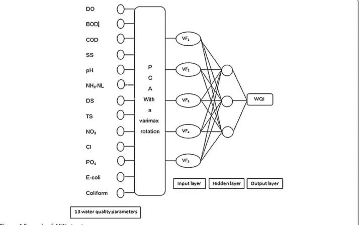
(i) An input layer which is connecting the input information to the network. In this assessment thirteen input nodes representing the thirteen water quality parameters were applied (DO, BOD, COD, SS, pH, AN, DS, TS, NO3, Cl-, PO4,E. coliand coliform). (ii) Hidden layer which is acting as the intermediate

computational layer. Multi-layer feed forward network formed by only one hidden layer. ANN models consist of the following set of equations:

Mb¼f½PPabRaŠ 1≤b≤B 1 ð4Þ

P represents the scaled input vector and M is output vector of the neurons contain in the hidden layer. The bias is set equal to 1.

(iii) Output layer is producing the desired output which is in this case the WQI following this equation:

Xc¼f½PPbcMbŠ 1≤k≤K ð5Þ

The coefficients Pab and Pbc in the summation, which

Many studies already emphasized the use of linear re-gression in apportionment of sources toward the de-pendable variables in their studies. Nonetheless, ANN application was yet to be explored. The aim of this method is to minimize the effect of multicollinearity and achieve better prediction model with minimum residual errors. The small number of input variables from APCS was combined with the ANN model to obtain high inter-pretability as the irrelevant and superfluous variables were excluded (Figure 4).

Results

Principle component scores (PCS)

The PCA showed that the two main PCs accounted for 45.13% of the total variance (PC1 21.40%; PC2 23.73%) for the overall observations. The larger variability graph for factor loading 1 and factor loading 2 were plotted to explain the variance. The 13 variables were well repre-sented on the plane.

The five VFs were generated after varimax rotation based on eigenvalues >1 (Kim and Mueller, [39]), (Figure 5). Eigenvalues and the corresponding factors were sorted by descending order and the initial variability was represented in percentage. The main approach of PCA is to reduce the number of variables by identifying the structure which cor-responded between variables and classify the new variables as shown in Figure 6. PCA is competent to extract latent

information and explains the structure of the data in detail (Wuet al., [40]). PCA after varimax rotation indicates five VFs with 79.41% of the total variability (Table 1).

Source apportioning by absolute principal component scores (APCS)

PCA aims to exclude redundant information from the original raw dataset by obtaining a small number of vari-ables. This is comprehensible especially for detailed ana-lysis such as modeling. Source apportioning are well known especially for air pollution and water quality data as it integrated with WQI although it is less documented in tropical regions. In air pollution studies, PCA and environmetric techniques are used extensively to deter-mine possible natural and anthropogenic contributions in the determination of total mass and concentration (Randolph et al., [41]). Therefore, the computation of APCS for receptor modeling or source apportioning for each observation is required.

APCS- MLR model

Basically MLR is based on a linear least-squares fitting process which requires a trace element or property to be determined for each source or source category in order to describe the old variables into new (Henry et al., [42]). Therefore, the PCA and MLR were combined in order to identify the potential pollution sources of the

Kuantan River Basin. Two basic types of receptor mod-els that are generally applied for source apportionment are chemical mass balance (CMB) and multivariate tech-niques (Gordon, [43]). Other than that, PCA also identi-fies tracers that represent specific sources and the

sources are selected as input (independent variables) to predict dependent variables (Morandi et al., [44]). MLR are used particularly to explain the relationship between the source apportionment generated by PC and their correlation to WQI values. Other than that, MLR also examines the relationship of each source to the depend-ant variable (WQI) with five VFs as independent variables. The source apportionment is a vital environ-metric technique as it estimates the contribution of identified sources to the concentrations of each param-eter (Simeonov et al., [35]). Sources of contributions were then calculated with APCS-MLR to identify main pollution origin in Kuantan River Basin after determining the number and characteristics of possible sources. The coefficient of determination (R2) is commonly used to

Figure 6Graph plotting after varimax rotation: (a) Fertilizer waste (VF1); (b) Surface runoff (VF2); (c) Anthropogenic input (VF3); (d) Chemical and mineral changes (VF4); (e) Erosion (VF5).

Figure 5Variables (PC1 and PC2: 45.13%) after varimax rotation.

Table 1 The variability of VFs

VF D1 D2 D3 D4 D5

Eigenvalue 4.213 2.656 1.249 1.184 1.022

Variability (%) 32.409 20.43 9.605 9.11 7.858

evaluate model performance (Pearson, [45]); however R2 is not a good comparison measurement of different model since R2 only provides how excellent the model fits the data not how well it performs on external data (Aertsen et al., [19]). Table 2 represents the MLR model and the goodness of fitting statistics.

Figure 7 shows the standardized coefficients of inde-pendent variable of the WQI linear regression model and the contribution for each pollutant.

Figure 8 shows the graph for calculated WQI and pre-dicted WQI. It is known that 19 observations from over-all observations were out from the range of upper and lower boundary (95% mean of the confidence interval).

Figure 9 illustrates the residual analysis of the actual and predicted WQI using APCS-MLR model. The results show the deficiency of the APCS-MLR model as the data set with great difference in the range of−6 to 6.

APCS-ANN

APCS-ANN is a comparatively new concept driven in river water quality modeling to allow non-linear rela-tionships between variables to be ‘learnt’ through repeated presentation of input–output data sets. The use of numerical models such as ANN provides powerful tools to stimulate complex natural resources manage-ment problems (Nikoloset al., [46]). Currently in envir-onmental modeling, the aid of ANN to achieve good estimation and better accuracy in simulation and fore-casting are beyond the typical model obtained when using entirely linear models. Other than that, ANN also allows one to resemble any mathematical function with absolute accuracy and used for non-linear regression be-tween different variables in a self optimizing way. ANN has been conveniently applied in river water quality study at Langat River, Malaysia (Juahir et al., [18]). Al-though PCA offered qualitative information about the major source of pollution to Kuantan River basin, it also provided the quantitative information on the pollutant contributor of each source types (Wuet al., [47]).

Figure 10 demonstrates the performance of the ANN model of Kuantan River Basin representing the training and testing based on actual WQI and predicted WQI.

Figure 11 represents the residual graph and shows the contrast of the actual and predicted WQI values. The re-sidual values for each observation were in the range of

−25 to 10.

Determination of appropriate model APCS-ANN model based on sensitivity analysis

Classical process-based modeling approaches can pro-vide good evaluations of water quality variables however the approach is too common to be applied directly with-out a lengthy data calibration process (Palani et al., [48]). Since APCS-ANN gives better accuracy compared to APCS-MLR model, therefore detailed analysis is required for assessment in order to identify the effect of input variables towards the output. Sensitivity analysis was performed on the data set using varimax factor as the input and WQI values as the output layer. For the entire created network, four hidden layers were used as it been selected in optimal architecture of the input parameters. This is important to mention as ANN net-works are sensitive to the number of hidden layer. Lesser

Table 2 Summary of regression of variable WQI

Goodness of fit statistics

Observations 275

Sum of weights 275

DF 269

R2 0.865

Adjusted R2 0.863

MSE 31.589

RMSE 5.62

AIC 955.454

SBC 977.155

Figure 7Standardized coefficients for each variable.

number of hidden nodes may result under fitting in the model (Doganet al., [49]).

The results depicted in Table 3 show models perform-ance evaluations of the effective parameters for forecast-ing WQI values. These models have been built through sensitivity analysis by removing one parameter or one model at a time. Sensitivity analysis is necessary to know how significant the excluded parameter or model would affect theR2values (Leeet al., [50]).

Discussion

Based on Figure 5, PCA was applied to the data set to compare the compositional pattern between the ana-lyzed water samples and to identify the factor that reflects with each other (Singhet al., [1]). PCA was per-formed on the raw dataset comprising all the 13 water quality parameters (DO, BOD, COD, SS, pH, NH3-NL, DS, TS, NO3, Cl-, PO4, E.coli, coliform) with 275 obser-vations to identify the pollution sources. PCA is able to describe the relationship between analytical variables than single analytical variable alone. VF1 (Eigenvalue 4.213) represents 21.40% of the total variability in one axis (VF1) comprising DO, AN and PO4. VF1 represents moderate loading matrix of coliform and E. coli. while DO was negatively correlated to AN and PO4 owing to the decrease of DO values in the increasing AN and

PO4inputs in the water body at Kuantan River. VF2 ex-plain DS, TS and Cl in new variable with strong factor loadings.

According to Table 1 and Figure 6a, DO, AN and PO4 were strongly correlated to VF1 (32.409% of variance) and a new variable termed as fertilizer waste which explains that NH4 likely to comes from the vicinity of animal farm and agricultural nonpoint source (Crowther et al., [51]; Singhet al., [52]; Songet al., [53]). Moderate loading of coliform andE. colisuggested minimum con-tribution of fecal pollution to the agriculture waste in Kuantan River Basin.

As shown in Table 1 and Figure 6b, surface runoff was named after VF2 (20.430% of variance) with high factor loadings for DS, TS and Cl-. While for VF3 (9.605% of variance) (Figure 6c) was strongly correlated with BOD and COD representing the influence of anthropogenic input typically organic pollution such as runoff from solids or waste disposal activities (Songet al., [53]). VF4 (9.110% of variance) and VF5 (7.858% of variance) were completely different from the other VFs owing to only one parameter that significantly related to their corre-sponding axis (Figure 6d and e). Thus, VF4 and VF5 were named as chemical and mineral changes (pH) and erosion (SS), respectively. The new variables created were further introduced to two different numerical mod-eling networks for WQI prediction and apportioning the sources that contribute to Kuantan River Basin.

In this study, factor scores from PCA after varimax ro-tation were used in receptor models development using MLR and ANN. Both models were further compared to Figure 9Residual between actual WQI and predicted WQI.

Figure 10Estimation of predicted WQI and actual WQI.

Figure 11Residual graph.

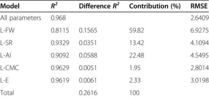
Table 3 The results of sensitivity analysis

Model R2 _DifferenceR2 _{Contribution (%) RMSE}

All parameters 0.968 2.6409

L-FW 0.8115 0.1565 59.82 6.9275

L-SR 0.9329 0.0351 13.42 4.1094

L-AI 0.9092 0.0588 22.48 4.5495

L-CMC 0.9629 0.0051 1.95 2.8014

L-E 0.9619 0.0061 2.33 3.0198

evaluate the performance on the data set. The use of PC based models was considered more dynamic, due to elimination of collinearity problems and prediction im-provement (Sousa et al., [8]). Moreover the utility of APCS that contain minimum input for both model com-pared to the raw data set was beneficial since it will in-crease the computational efficiency and interpretability and reduce the noise and redundancy for the model.

Referring to Table 2, the R2 value for APCS-MLR model in this study is 0.87 and the model indicates that 87% variability of WQI explained by the five independ-ent variables used in the model. While for adjustedR2it is always less thanR2and increases only if the new term improve the model (Aertsen et al., [19]). Mean Square Error (MSE) and Root Mean Square Error (RMSE) measure residual errors which give estimation of the mean difference between observed and modeled values of WQI. The minimum value of MSE for APCS-MLR result (Table 2) corresponds to best network topology (Sousaet al., [8]).

Best model performance are Akaike_’s Information Cri-teria (AIC) and Schwarz Bayesian CriCri-teria (SBC) values and R2 and adjusted R2 values closet to unity (Aertsen et al., [19]). In general AIC, Bayesian Information Criteria (BIC) and SBC estimate the loss of accuracy caused by accounting a number of parameters and the number of data points used in its calibration. The small difference for AIC and SBC values signify that MLR was a fit method for WQI prediction. The high and great difference between values of AIC and SBC from the APCS-MLR model in this study (Table 2) indicate that the model has inadequacy in terms of fitness and robustness.

Based on Figure 7, fertilizer waste accounts as the highest pollution contributor to Kuantan River Basin while the next main contributor was anthropogenic in-put that may come from the vicinity area of Kuantan River basin. The negative standardized coefficient of in-dependent variables (fertilizer waste, surface runoff, an-thropogenic input and erosion) is based on negatively correlation to WQI values (as all the four independent variable decrease, WQI value increase). As shown in Figure 8, this proved that this model is able to predict WQI values from the varimax factor of PCA with negli-gible precision. In Figure 9, the verification and applic-ability of the model was influenced by the existence of the outlier observations as shown also in Figure 8.

APCS-ANN (WQI) was developed to investigate which pollution patterns contribute most to the Kuantan River Basin. Previously five VFs were generated from PCA after varimax rotation and the VFs were used as input param-eter for ANN model. The five input paramparam-eters were fertilizer waste, surface runoff, and anthropogenic input, chemical and mineral changes and erosion and WQI as output. Based on Figure 10, APCS-ANN model developed

produced good accuracy with R2value, 0.9680 (Table 3-all input) for both training and testing sets with 66.76% and 33.33% of the overall data set. The correlation coeffi-cients for both set approach to 1 which further explain the network output almost equal to the output (Garcia and Shigidi, [54]) and high accuracy for the cross validation with minimum value of RMSE (Rossel and Behrens, [14]). As shown in Figure 9 the predicted WQI values from the training set are able to follow the pattern recognized by the training set and produce high reliability and goodness-of-fit. The RMSE was chosen as main criteria to determine model performance. The APCS-ANN model has low value of RMSE (2.6409) compared to the APCS-MLR model (5.6200).

As shown in Figure 11, although the range is quite broad, the residual data were evenly distributed in the zero values. Only few outliers and extreme values were identi-fied which only contribute minimum error to model ro-bustness. As shown in Table 3, APCS-ANN model with all input parameters were selected as the most appropriate model for WQI forecasting with high R2is (0.9680) and low RMSE (2.6409) as compared to other models. From the sensitivity analysis, the highest pollutant that contribu-ted to Kuantan River Basin (WQI variation) was identified. Fertilizer waste (L-FW) accounted as the main pollution contributor (high percentage contribution, 59.82%) due to the exclusion of the parameters results in reduction ofR2 (0.8115) and high RMSE (6.9275) which signify the model. Anthropogenic input (L-AI) was identified as the second pollution contributor (percentage contribution, 22.48%), R2(0.9092) and RMSE (4.549) followed by surface runoff (L-SR), erosion (L-E) and lastly chemical and mineral changes (L-CMC) which were the least contributors as the inputs influencing the APCS-ANN model performance.

APCS-MLR in apportionment of sources affecting water quality reveals that industrial discharge contributed the highest pollutant of ammonia observed (Dalalet al., [55]). However, application of in APCS-ANN Kuantan River Basin indicates a better accuracy than APCS-MLR shows that this is not an industrialized region yet it is governed by agriculture (palm oil plantation); thus fertilizer seems to be the major contributor. Therefore this study is expected to establish the baseline comparison in identify-ing the pollution contribution for future water resources and management.

Conclusion

changes to the field areas. From the results stated above, it is shown that ANN gives better accuracy as compared to MLR technique for WQI forecasting. Moreover ANN also capable to stimulate the complex relationship between the data set and consequently is able to justify the water quality puzzles. By using PCA, main pollution contributors to the basin were justified without eliminating any data and parameters. Moreover due to non-linearities of dependent variables in this study and the intricate associations between water quality parameters and WQI values, APCS-ANN model is able to justify and predict the WQI values at Kuantan River Basin. In this sense, APCS methods proved con-stitute recommended tools for more comprehensible of large volume data sets especially in environmental monitoring studies. Thus, the prediction of WQI values using APCS-ANN model can be used for environmen-tal monitoring agencies in Malaysia to reduce the mon-itoring and chemical analysis cost as only significant parameters (DO, AN and PO4) will further used for monitoring purposes. The model gives efficient compu-tational judgments.

Competing interests

The authors declare that they have no competing interests.

Authors’contributions

Nasir MFM, carried out the environmental modeling studies, assisting in the writing, data analyzing, drafted and submission of the manuscript. Zali AM, carried out the environmental modeling studies, assisting in the writing, data analyzing and drafted the manuscript. Juahir H, carried out the

environmental modeling studies, participated in sequence alignment and reviewing the manuscript. Hussain H, contributed in the data and landuse map of the manuscript. Zain SM, participated in the reviewing of the manuscript. Ramli N., contributed in the water quality data for the manuscript. All authors read and approved the final manuscript.

Acknowledgements

The authors would like to thank the Department of Environment, Malaysia, for providing the data used in this study and colleagues who had given inspirational help at readings and sharing their wise ideas for the completion of this manuscript.

Author details

1_{Department of Environmental Sciences, Faculty of Environmental Studies,}

UPM Serdang, Selangor, Malaysia.2Department of Environment, Federal Government Administrative Centre, Environment Institute of Malaysia, Putrajaya, Malaysia.3Department of Chemistry, Faculty of Science, Universiti Malaya, Kuala Lumpur, Malaysia.4_{Surface Water Monitoring Unit, Water and}

Marine Division, Department of Environment Malaysia, Federal Government Administrative Centre, Putrajaya, Malaysia.

Received: 28 November 2012 Accepted: 28 November 2012 Published: 10 December 2012

References

1. Singh KP, Malik A, Mohan D, Sinha S:Multivariate statistical techniques for the evaluation of spatial and temporal variations in water quality of Gomti River (India)-a case study.Water Res2004,38:3980–3992. 2. DID:Annual Report of Department of Irrigation and Drainage. Kuala Lumpur:

Ampang; 2001.

3. Ibrahim R:Proceedings National Conference on Sustainable River Basin Management in Malaysia: 13–14 November 2001. Kuala Lumpur.

Malaysia; 2001.

4. Department of Environment (DOE):Malaysia Environmental Quality Report.InMinistry of Natural Resources and Environment Malaysia; 2007. http://www.doe.gov.my/portal/publication-2/.

5. Massart DL, Vandeginste BGM, Deming SN, Michotte Y, Kaufman L: Chemometrices: A Text book. Amsterdam: Elsevier; 1988.

6. Department of Environment (DOE):Malaysia Environmental Quality Report.InMinistry of Natural Resources and Environment Malaysia; 1997. http://www.doe.gov.my/portal/publication-2/.

7. Bandyopadhyay G, Chattopadhyay S:Single layer artificial neural network models versus multiplelinear regressio model in forecasting the time series of total ozone.Int J Environ Sci Technol2007,4:141–149. 8. Sousa SIV, Martins FG, Alvim-Ferraz MCM, Pereira MC:Multiple linear

regression and artificial neural networks based on principal components to predict ozone concentration.Environ Model Software2007,22:97–103. 9. Chaloulakou A, Saisana M, Spyrellis N:Comparative assessment of neural networks and regression models for forecasting summertime ozone in Athens.Sci Total Environ2003,313:1–13.

10. Jahandideh S, Jahandideh S, Asadabadi EB, Askarian M, Movahedi MM, Hosseini S, Jahandideh M:The use of artificial neural networks and multiple linear regression to predict rate of medical waste generation. Waste Manag2009,29:2874–2879.

11. Ogwueleka TC, Ogwueleka FN:Modelling energy content of municipal solid waste using artificial neural network.Iran J Environ Health Sci Eng 2010,7(3):259–266.

12. Thompson ML, Reynolds J, Cox LH, Guttorp P, Sampson PD:A review of statistical methods of the meteorological adjustment of tropospheric ozone.Atmos Environ2001,35:617–630.

13. Gutierrez-Estrada JC, Bilton DT:A heuristic approach to predicting water beetle diversity in temporary and fluctuating waters.Ecol Model2010, 221:1451–1462.

14. Rossel RAV, Behrens T:Using data mining to model and intepret soil diffuse reflectance spectra.Geoderma2010,158:46–54.

15. Wu J, Mei J, Wen S, Liao S, Chen J, Shen Y:A self-adaptive genetic algorith-artificial neural network algorith with leave-one-out cross validation for descriptor selection in QSAR study.J Comput Chem2010, 31:1956–1968.

16. Mirsepassi A:Application of intelligent system for water treatment plant operation.Iranian J Env Health Sci Eng2004,1(2):51–57.

17. French JL, Krajewski WF, Cuykendall RR:Rainfall forecasting in space and time using a neural network.Journal Hydrology1992,137:1–31.

18. Juahir H, Zain SM, Toriman ME, Mokhtar M, Man HC:Application of artificial network models for predicting water quality index.Jurnal Kejuruteraan Awam2004,16:42–55.

19. Aertsen W, Kint V, Orshoven JV, Ozkan K, Muys B:Comparison and ranking of different modelling techniques for prediction of site index in mediterranean mountain forests.Ecol Model2010,221:1119–1130. 20. Department of Environment (DOE):Local Plan 2004–2015.InMinistry of

Natural Resources and Environment Malaysia. 2006. http://www.doe.gov.my/ portal/publication-2/.

21. Department of Environment (DOE):Ministry of Natural Resources and Environment Malaysia. 2004. http://www.doe.gov.my/portal/publication-2/. 22. Aiken RS, Leigh CH, Leinbach TR, Moss MR:Development and Environment

in Peninsular Malaysia. Singapore: Mc Graw-Hill International Book Company; 1982.

23. Zhou F, Liu Y, Guo H:Application of multivariate statistical methods to water quality assessment of the water courses in north western new territories.Hong Kong. Environ Monit Assess2007,132:1–13.

24. Krishna AK, Satyanarayanan M, Govil PK:Assessment of heavy metal pollution in water using multivariate statistical techniques in an industrial area: a case study from Patancheru, Medak District. Andhra Pradesh, India.J Hazard Mater2009,167:366–373.

25. Felipe-Sotelo JMA, Carlosena A, Tauler R:Temporal characterisation of river waters in urban and semi-urban areas using physico-chemical parameters and chemometric methods.Analytica Chemica Acta2007, 583:128–137.

26. Camdevyren H, Demyr N, Kanik A, Keskyn S:Use of principal component scores in multiple linear regression models for prediction of Chlorophyll-ain reservoirs.Ecol Model2005,181:581–589.

28. Vega M, Pardo R, Barrado E, Deban L:Assessment of seasonal and polluting effects on the quality of river water by exploratory data analysis.Water Res1988,32:3581–3592.

29. Helena B, Pardo R, Vega M, Barrado E, Fernandez JM, Fernandez L: Temporal evolution of groundwater composition in an alluvial aquifer. Water Res2000,34:807–816.

30. Wunderlin DA, Diaz MP, Ame MV, Pesce SF, Hued AC, Bistoni MA:Pattern recognition techniques for the evaluation of spatial and temporal variations in water quality. A case study: Suquia river basin (Cordoba-Argentina).Water Res2001,35:2881–2894.

31. Sarbu C, Pop HF:Principal component analysis versus fuzzy principal component analysis a case study: the quality of danube water (1985–1996).Talanta2005,65:1215–1220.

32. Liu CW, Lin KH, Kuo YM:Application of factor analysis in the assessment of groundwater quality in a blackfoot disease area in Taiwan.Sci Total Environ2003,313:77–89.

33. Swietlicki E, Krejei R:Source characterisation of the Central European atmospheric aerosol using multivariate statistical methods.Nucl Instrum Methods Phys Res, Sect B1999,109–110:519–525.

34. Fung YS, Wong LWY:Apportionment of air pollution sources by receptor models in Hong Kong.Atmos Environ2000,29:2041–2048.

35. Simeonov V, Stratis JA, Samara C, Zachariadis G, Voutsa D, Anthemidis A, Sofoniou M, Kouimtzis T:Assessment of the surface water quality in Northern Greece.Water Res2003,37:4119–4224.

36. Simeonov V, Simeonova P, Tzimou-Tsitouridou R:Chemometric quelity assessment of surface waters: two case studies.Chem Eng Ecol2004, 11:450–460.

37. Thurston GD, Spengler JD:A quantitative assessment of source contributions to inhalable particulate matter pollution in metropolitan Boston atmospheric environment - part A.General Topics1985,19:9–25. 38. Moatar F, Fessant F, Poirel A:pH modelling by neural networks.Application

of control and validation data series in the Middle Loire river. Ecol Model1999, 120:141–156.

39. Kim JO, Mueller CW:Introduction to Factor Analysis: What it is and how to do it, Sage University Paper series on quantitative applications in the social sciences series. Beverly Hills, CA: Sage Publications; 1978.

40. Wu M, Wang Y, Sun C, Wang H, Dong J, Yin J, Han S:Identification of coastal water quality by statistical analysis methods in Daya Bay, South China Sea.Mar Pollut Bull2010, Article in Press.

41. Randolph K, Larsen I, Baker JE:Source apportionment of polycyclic aromatic hydrocarbons in the urban atmosphere: a comparison between three methods.Environ Sci Technol2003,37:1873–1881.

42. Henry CR, Lewis CW, Hopke PK, Williamson HJ:Review of receptor model fundamentals.Atmos Environ1984,18:1507–1515.

43. Gordon GE:Receptor models.Environ Sci Technol1988,22:1132–1142. 44. Morandi MT, Daisey JM, Lioy PJ:Development of a modified factor

analysis/multiple regression model to apportion suspended particulate matter in a complex urban airshed.Atmos Environ1987,21:1821–1831. 45. Pearson K:Regression, heredity and panmixia. In: mathematical

contributions to the theory of evolution.Philos Trans R Soc Lond1896, Set. A 187:253–318.

46. Nikolos IK, Stergiadi I, Papadopoulo MP, Karatzas GP:Artificial neural networs as an alternative approach to groundwater numerical modelling and environmental designs.Hydrological Procesess2008,22:3337–3348. 47. Wu B, Zhao D, Zhang Y, Zhang X, Cheng S:Multivariate statistical study

of organic pollutants in Nanjing reach of Yangtze River.J Hazard Mater 2009,169:1093–1098.

48. Palani S, Liong SY, Tkalich P:An ANN application for water quality forecasting.Mar Pollut Bull2008,56:1586–1597.

49. Dogan E, Sengorur B, Koklu R:Modelling biological oxygen demand of the Melen River in Turkey using an artificial neural network technique.

J Environ Manage2009,90:1229–1235.

50. Lee JHW, Huang Y, Dickman M, Jayawardena AW:Neural network modelling of coastal algal blooms.Ecol Model2003,159:179–201. 51. Crowther J, Kay D, Wyer MD:Relationships between microbial water

quality and environmental conditions in coastal recreational waters: The Flyde Coast.UK. Water Res2001,35:4029–4038.

52. Singh KP, Malik A, Singh VK, Mohan D, Sinha S:Chemometric analysis of groundwater quality data of alluvial aquifer of Gangetic plain. North India. Anlytica Chimica Acta2005,550:82–91.

53. Song MW, Huang P, Li F, Zhang H, Xie KZ, Wang XH, He GX:Water quality of a tributary of the Pearl River, the Beijing, Southern China: implications from multivariate statistical analyses.Environ Monit Assess 2011,172:589-603.

54. Garcia LA, Shigidi A:Using neural networks for parameter estimation in ground water.Journal of Hydrology2006,318:215–231.

55. Dalal SG, Shirodkar PV, Verlekar XN, Jagtap TG:Apportionment of sources affecting water quality: case study of Kandla Creek, Gulf of Katchchh. Environ Forensics2009,10:101–106.

doi:10.1186/1735-2746-9-18

Cite this article as:Nasiret al.:Application of receptor models on water quality data in source apportionment in Kuantan River Basin.Iranian Journal of Environmental Health Science & Engineering20129:18.

Submit your next manuscript to BioMed Central and take full advantage of:

• Convenient online submission

• Thorough peer review

• No space constraints or color figure charges

• Immediate publication on acceptance

• Inclusion in PubMed, CAS, Scopus and Google Scholar

• Research which is freely available for redistribution