Frequency- or amplitude-dependent effects of the Atlantic meridional overturning on the tropical Pacific Ocean

www.ocean-sci.net/5/293/2009/

© Author(s) 2009. This work is distributed under the Creative Commons Attribution 3.0 License.

Ocean Science

Frequency- or amplitude-dependent effects of the Atlantic

meridional overturning on the tropical Pacific Ocean

G. J. van Oldenborgh1, L. A. te Raa2,*, H. A. Dijkstra2, and S. Y. Philip1 1_{Royal Netherlands Institute of Meteorology, De Bilt, The Netherlands}

2_{Institute for Marine and Atmospheric research Utrecht, Utrecht University, Utrecht, The Netherlands} *_{currently at: Netherlands Organisation for Applied Scientific Research TNO, The Hague, The Netherlands}

Received: 2 February 2009 – Published in Ocean Sci. Discuss.: 27 February 2009 Revised: 19 June 2009 – Accepted: 14 July 2009 – Published: 27 July 2009

Abstract. Using the ECHAM5/MPI-OM model, we study

the relation between the variations in the Atlantic meridional overturning circulation (AMOC) and both the Pacific sea sur-face temperature (SST) and the El Ni˜no-Southern Oscillation (ENSO) amplitude. In a 17-member 20C3M/SRES-A1b en-semble for 1950–2100 the Pacific response to AMOC varia-tions on different time scales and amplitudes is considered. The Pacific response to AMOC variations associated with the Atlantic Multidecadal Oscillation (AMO) is very small. In a 5-member hosing ensemble where the AMOC collapses due to a large freshwater anomaly, the Pacific SST response is large and in agreement with previous work. Our results show that the modelled connection between AMOC and ENSO de-pends very strongly on the frequency and/or the modelled amplitude of the AMOC variations. Interannual AMOC vari-ations, decadal AMOC variations and an AMOC collapse lead to entirely different responses in the Pacific Ocean.

1 Introduction

Decadal to multidecadal modulations of the amplitude of ENSO have been found in observations of SST, sea level pressure and rainfall (e.g., Torrence and Webster, 1999). Recently, multidecadal SST variations associated with the AMO have been suggested as a possible explanation for low-frequency ENSO variability (Dong et al., 2006; Timmer-mann et al., 2007). The large-scale SST pattern of the AMO in the North Atlantic is thought to be related to multidecadal

Correspondence to:

G. J. van Oldenborgh (oldenborgh@knmi.nl)

variations of the AMOC (Delworth and Mann, 2000; Knight et al., 2005; Dijkstra et al., 2006). In particular, a positive AMO (relatively high North Atlantic SSTs) has been found to be associated with a strong AMOC (Knight et al., 2005), possibly with a phase lag between the maximum AMO and the maximum AMOC (Dijkstra et al., 2006). Using a cou-pled ocean-atmosphere GCM, Dong et al. (2006) suggest that latent heat anomalies associated with a positive phase of the AMO lead to a deeper equatorial thermocline in the Pa-cific through anomalous easterly winds. This in turn reduces ENSO variance in the model. Sutton and Hodson (2007) also show that large-scale temperature anomalies in the North At-lantic Ocean can affect the tropical Pacific region.

reduction typically induced by large freshwater anomalies. The same holds for observations, considering the AMO in-dex as a proxy of AMOC variability.

Chang et al. (2008) showed that in the first stage of hosing-experiments changes in tropical Atlantic SST are relatively small. The second stage starts after reaching a threshold in the AMOC beyond which more drastic warming takes place in this region. This threshold is reached when the strength of the AMOC is reduced to that of the wind-driven subtrop-ical cell. Here we follow up on this study with the ques-tion whether the response of the Pacific to a collapse to the AMOC can be compared to that of interannual to multi-decadal natural variability in the AMOC.

We compare the effect of AMOC changes on the tropical Pacific SST and ENSO amplitude using two ensembles of runs performed with the coupled ECHAM5/MPI-OM model. Using a 17-member ensemble of climate runs for the period 1950–2100 under the 20C3M/SRES-A1b scenario, we first study the response of the tropical Pacific to AMO and re-lated AMOC variations. Next, the tropical Pacific response to a forced collapse of the AMOC is investigated in a 5-member ensemble performed with the same model for the period 2000–2100.

2 Model, simulations and observational datasets

All experiments are part of the ESSENCE project (Sterl et al., 2008) and have been conducted with the ECHAM5/MPI-OM coupled climate model, which is described by Roeckner et al. (2003) and Marsland et al. (2003). Although the model suf-fers from a too pronounced and too far westward extending Pacific equatorial cold tongue, the simulated ENSO as well as the thermohaline circulation are quite reasonable (Mars-land et al., 2003; Jungclaus et al., 2006; van Oldenborgh et al., 2005). The model is run in the configuration used for the AR4 climate scenario runs, with a horizontal resolution of T63 and 31 vertical hybrid levels in the atmosphere and an average horizontal resolution of 1.5◦_{and 40 vertical layers in} the ocean.

The standard ensemble consists of 17 runs over the period 1950–2100. Greenhouse gas and tropospheric aerosol con-centrations are specified from observations for 1950–2000 and follow the SRES-A1b scenario for 2001–2100. The runs are initialised from the year 1950 of a 20th century simula-tion, with the atmospheric temperature perturbed by adding Gaussian noise with an 0.1◦C amplitude. The large ensem-ble allows a clean separation of internal variability and the forced signal. The latter is well-represented by the ensemble mean, the former by anomalies with respect to the ensemble mean.

The hosing ensemble consists of 5 members, each ini-tialised from the year 2000 from a different member of the standard ensemble. A 1 Sv freshwater anomaly was added in an area near Greenland from the end of year 2000 onwards.

Apart from this additional freshwater input, the forcing is the same as in the standard ensemble. With the hosing ensemble the Pacific response to a large, long lasting variation in the AMOC is investigated, whereas with the standard ensemble we study the influence of relatively small amplitude natural variability in the AMOC on the Pacific.

To compare with observations we use the HadSST2 SST analysis (Rayner et al., 2006) and the HadISST1 SST recon-struction (Rayner et al., 2003). For the AMO teleconnections over land we used the CRU TS 3 datasets. We do not use data before 1900 because of the large uncertainties.

3 Results

The AMO index has been calculated as the average of monthly SST anomalies with respect to the ensemble mean over the North Atlantic north of 25◦N (75◦W–7◦W, 25◦N– 60◦_{N). This differs from the usual definitions in two aspects.} First, the tropical Atlantic has been omitted. This region is influenced by well-known ENSO teleconnections (Czaja et al., 2002). Even with a 5-yr running mean, the correla-tion between tropical North Atlantic SST (EQ–20◦N) and the Ni˜no 3.4 index is 0.48±0.04 in the model and 0.21±0.48 in the observations (here and in the following the errors rep-resent a symmetrical 2σ (95%) uncertainty range). As we want to study teleconnections from the North Atlantic to the ENSO region, inclusion of the tropical Atlantic would con-fuse the issue. The effect of the different domain size in the AMO index is not large; in the ESSENCE ensemble the av-erage from the equator to 60◦N is strongly correlated to the average from 25◦N–60◦N,r=0.82±0.04 with a 5-yr run-ning mean.

The second difference concerns the subtraction of the triv-ial effects of global warming on an SST average (cf. Tren-berth and Shea, 2006). In the large ESSENCE ensemble subtracting the ensemble mean easily separates the internal variability from the externally forced temperature rise. In the observations, this is not so straightforward. Guided by the observation that in the model the internal AMO and global mean temperature fluctuations are very weakly correlated (r=0.25, see also van Oldenborgh et al., 2009) we define the AMO index in the observations as the averaged SST in the North Atlantic minus the regression of this SST on global mean temperature. This index is very similar to the one de-fined by Trenberth and Shea (2006).

(a)

-0.4 -0.2 0 0.2 0.4

1960 1980 2000 2020 2040 2060 2080 2100 2

1

0

-1

-2

AMO [K]

AMOC [Sv]

ESSENCE 4 AMO index

ESSENCE 4 AMOC

(b)

-0.4 -0.2 0 0.2 0.4

1860 1880 1900 1920 1940 1960 1980 2000 2

1

0

-1

-2

AMO [K]

AMOC [Sv]

AMO HadSST2

(c)

-0.2 0 0.2 0.4 0.6

-20 -15 -10 -5 0 5 10 15 20

correlation

lag [yr], positive: AMOC leading AMO

(d)

0 0.1 0.2 0.3

100 50

20 10

5 2

power [K

2]

AMO ESSENCE

AR(1)

(e)

0 0.1 0.2 0.3

100 50

20 10

5 2

power [K

2]

AMO HadSST2 AR(1)

(f)

0 0.1 0.2 0.3

100 50

20 10

5 2

power [Sv

2]

AMOC ESSENCE AR(1)

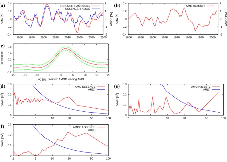
Fig. 1. (a)AMO index (red) and maximum AMOC at 35◦N (blue) for standard ensemble member 4. (b)AMO index in the observations

(HadSST2).(c)Lag correlation between maximum AMOC at 35◦N and the AMO index. For positive lags the AMOC is leading. The green

band indicates the 95% confidence interval based on a decorrelation time scale of 5 years.(d)Spectrum of the AMO index in the ESSENCE

experiments, the green line indicates the 95% upper bound of an AR(1) process with the same autocorrelation at lag 1 year.(e)Same for the

observations.(f)Spectrum of the AMOC index in the model.

The maximum AMOC at 35◦N varies about 1 Sv around the ensemble mean (Fig. 1a). As there is only one 5-yr period of observations at 26.5◦N, and reanalyses vary wildly, we cannot compare this to observations.

The multidecadal variability in the modelled AMO and AMOC has a broad peak at about 20 years. In the AMOC there is a second peak at 50 years. Both spectra show a long tail with higher periods (Figs. 1d, f). This is very similar to what was found by Dong and Sutton (2005) in the HadCM3 model, and by Keenlyside et al. (2008) in another configura-tion of the MPI model. Jungclaus et al. (2005) found a peak at 70–80 years in a control run of a model configuration that is more similar to the one used in ESSENCE. These long periods are difficult to detect in the 150-year transient runs described here. The uncertainties on the spectrum of the ob-served AMO (Fig. 1e) are very large (almost as large as the value in this spectrum). Within these large uncertainties the observations and model agree reasonably well.

The correlation between the AMO index and the AMOC for all standard ensemble members together is 0.55, with the overturning leading by about 2 years (Fig. 1c). Hence there is a significant relation between the AMO and the multidecadal AMOC variability in this model. The fact that the AMO index lags the maximum AMOC is in agreement with the mechanism of the AMO as suggested in Te Raa and Dijkstra (2002). As the correlation between the AMO index and the AMOC is 0.55 we investigate the response of the Pacific to changes in both the AMO and the AMOC.

(a)

model regression SST on AMO, 5−yr running mean

(b)

obs regression SST on AMO, 5−yr running mean

(c)

model regression SST on AMOC, 5−yr running mean

(d)

model regression SST on AMO, annual mean

(e)

obs regression SST on AMO, annual mean

(f)

model regression SST on AMOC, annual mean

Fig. 2. (a)Regression [K/K] of model SST on the model AMO index (5-yr running mean, anomalies w.r.t. the ensemble mean). (b)

Regression [K/K] of HadISST1 SST on the HadSST2 AMO index (5-yr running mean, regression onTglobal subtracted). (c)Regression

[K/Sv] of SST on maximum AMOC at 35◦N (5-yr running mean).(d-f)As(a-c)but for annual means. Areas for which thep-value exceeds

(a)

model correlation T2m with AMO, 5−yr running mean

(b)

obs correlation T2m/SST with AMO, 5−yr running mean

(c)

model correlation precip with AMO, 5−yr running mean

(d)

obs correlation precip with AMO, 5−yr running mean

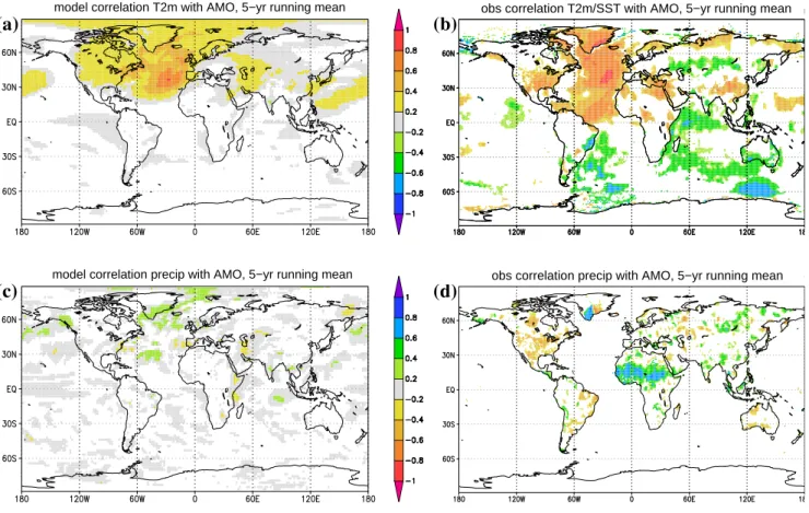
Fig. 3. (a)Correlation of model 2m-temperature on the model AMO index (5-yr running mean, anomalies w.r.t. the ensemble mean). (b)

Correlation of HadISST1 SST and CRU TS3 T2m on the HadSST2 AMO index (5-yr running mean, regression onTglobalsubtracted).(c)

and(d)Same for precipitation. Shading as in Fig. 2.

AMO in this model (Figs. 3c,d, cf. Biasutti et al., 2006). The teleconnection to the Caribbean Sea (10◦_N–20◦_{N, 90}◦_W– 60◦_{W) is also weaker in the model (r=0.13±0.06) than in} the observation (0.47±0.28), although the uncertainty ranges overlap. Teleconnections to annual mean land surface air temperature are similar to the observed ones, with the largest signal in the eastern half of the US with correlations ofr≈0.3 (Figs. 3a,b, see also Trenberth and Shea, 2006). The signifi-cance of the observed teleconnections was computed assum-ing a decorrelation scale equal to the 5 years of the runnassum-ing mean.

Neither in the observations nor in the standard ensemble there is a statistically significant response of tropical Pacific SST to the AMO (Fig. 2a,b). In the model, the correlation between 5-yr running means of the AMO and the Ni˜no 3.4 index is less than 0.22 for any lag varying from 0 to 20 years (AMO leading). Due to the large number of ensemble mem-bers, the statistical errors on this are much smaller than on the correlation in the observations,r=−0.20±0.29 at lag zero.

To study the relation between Pacific SST and the AMOC directly, we also computed the correlation between 5-yr

running means of the Ni˜no 3.4 index and the maximum AMOC at 35◦_{N. These correlations are even lower, with} maxima less than 0.1 for lags with the AMOC leading. The SST response to AMOC variations is indeed mostly confined to the North Atlantic (Fig. 2c), with no significant correla-tions in the equatorial Pacific.

(a)

0 5 10 15 20 25 30

1960 1980 2000 2020 2040 2060 2080 2100

AMOC [Sv]

Hosing Standard

(b)

regression SST on AMOC, 5-yr running mean

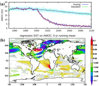
Fig. 4. (a)Maximum AMOC at 35◦N [Sv] of all hosing ensemble members (dots), together with their ensemble mean and 5-yr

run-ning mean. The standard ensemble is given for comparison. (b)

Regression of the difference in SST between the hosing and

stan-dard runs on the difference in maximum AMOC at 35◦N [K/Sv]

for 2000–2050. A 5-yr running mean has been applied to the data before regressing. Shading as in Fig. 2.

Having found no significant correlation between decadal AMOC variability and the mean temperature of the ENSO region, we turn to ENSO amplitudes. The lagged correlation between a 15-yr running standard deviation of Ni˜no 3.4 and the 5-yr running mean of maximum AMOC at 35◦N is at most−0.2 with the AMOC leading (not shown). A similar correlation with the AMO index is not statistically significant at the 95% level for any lag up to 20 years (AMO leading). From these results we conclude that in the standard ensem-ble, the AMO-related AMOC variability has no significant effects on ENSO amplitudes either.

In the hosing ensemble, the AMOC collapses to about 3 Sv in the year 2100 (Fig. 4a). As the AMOC also de-creases in the standard ensemble (Fig. 4a), and greenhouse gases are taken from the A1b scenario in the hosing runs, we compute the effect of AMOC decrease induced by the freshwater anomaly itself as the regression of the difference of hosing and standard runs with respect to the difference in AMOC strengths, i.e. the regression ofThosing−Tstandon

9_hosingmax −9_standmax. In general, the strongest response is found on the Northern Hemisphere (Fig. 4b). With statistically sig-nificant regression coefficients exceeding 0.03 K/Sv there is also a clear response in the equatorial Pacific SST. This SST response gives rise to a precipitation response that is global in nature and resembles the well-known ENSO teleconnec-tion pattern (not shown). The response of global SST (and of the tropical Pacific SST in particular) in the hosing ensem-ble is thus very different from that in the standard ensemensem-ble (compare Figs. 2b and 4b).

(a)

-2 -1.5 -1 -0.5 0 0.5 1 1.5

1960 1980 2000 2020 2040 2060 2080 2100

SSTa [K]

East Pacific SSTa

(b)

-2.5 -2 -1.5 -1 -0.5 0 0.5

1960 1980 2000 2020 2040 2060 2080 2100

SSTa [K]

Caribean SSTa

(c)

-30. -20. -10. 0. 10. 20.

1960 1980 2000 2020 2040 2060 2080 2100

taux [mPa]

Central America zonal wind

Fig. 5. Difference between ensemble mean values of hosing and standard ensembles (for 1950–2000, the difference between the mean of the first five members the ensemble mean of the

stan-dard ensemble). (a) Annual mean SST [◦C] (blue) and 5-yr

running mean (red) averaged over the eastern Pacific (150◦W–

90◦W, 10◦S–10◦N).(b)Annual mean SST (◦C) averaged over the

Caribbean (90◦W–60◦W, 10◦N–20◦N).(c)Annual mean zonal

wind stress (Pa) averaged over Central America (100◦W–75◦W,

5◦N–20◦N).

Drijfhout et al. (2008) found a similar dichotomy between oceanic wind- en density driven aspects of the AMOC in the CCSM 1.4 model, with the wind-driven overturning circu-lation responsible for most of the variability and almost en-tirely restricted to the northern hemisphere, whereas the de-crease due to global warming extends south over the equator. In the hosing ensemble, it takes about 10 years after the start of the freshwater anomaly before a significant change in SST in the tropical Pacific occurs (Fig. 5a). In fact, cool-ing only reaches the tropical Pacific after havcool-ing reached the Caribbean (Fig. 5b). Except for this time delay, the response is completely linear. Once the temperature in the Caribbean starts to drop, an atmospheric anticyclone develops over this region (not shown), and the easterly trade winds over central America intensify (Fig. 5c), thereby cooling the equatorial Pacific.

a

b

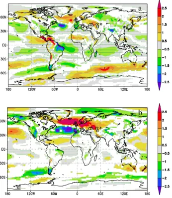
Fig. 6. (a)Regression of the difference in zonal wind stress between the hosing and standard ensembles on the difference in maximum

AMOC at 35◦N [mPa/Sv].(b)Regression of anomalies (w.r.t. the

ensemble mean) of zonal wind stress on maximum AMOC at 35◦N

[mPa/Sv] for all standard ensemble members. In both panels a 5-yr running mean has been applied to the data before regressing. Shad-ing as in Fig. 2.

to AMOC changes associated with the AMO is crucially dif-ferent (Fig. 6b) from that in (Fig. 6a) as there is no signature of an atmospheric bridge connecting the Atlantic and Pacific Oceans.

Chang et al. (2008) report on a similar delay in the GFDL model, but in effects of a reduction of the AMOC on the equatorial Atlantic. In that model the meridional overturn-ing has weakened so far after 20 years that warm subsurface water flows southward rather than northward in the thermo-cline at 8◦_{N. This warm water suppresses the annual} cool-ing in the equatorial Atlantic Ocean in July–September. In the ECHAM5/MPI-OM model this happens after just over 10 years, see Figs. 7a, b, at the same time as the warming of the Caribbean, the zonal wind stress change over Central America, and the teleconnection to SST in the East Pacific (Figs. 5a–c). The natural variability in the AMOC does not reach the point in which the annual mean transport becomes southward (Fig. 7a).

In Fig. 8 the evolution of the SST difference between the hosing and standard ensemble is shown. The cooling signal propagates along the subtropical gyre and has reached the

(a)

-4.0 -2.0 0.0 2.0 4.0 6.0

1960 1980 2000 2020 2040 2060 2080 2100

NSTC [Sv]

Hosing Standard

(b)

26. 27. 28. 29. 30.

1960 1980 2000 2020 2040 2060 2080 2100

SST [Celsius]

Equatorial Atlantic, hosing Equatorial Atlantic, standard

Fig. 7. (a)Annual mean northward flow through 7.5◦N between 100 m and 400 m. The fluctuations of the standard ensemble are

in-dicated by dots.(b)July–September SST in the Equatorial Atlantic.

Caribbean Sea in 2015. The final cooling pattern is similar to the mean AOGCM signal in Stouffer et al. (2006). Note that their Fig. 14 shows that simpler models do not reproduce the cooling signal in the Caribbean.

The cooling of the Caribbean sets up the atmospheric bridge, which causes cooling in the East Pacific. At the same time the warm water flows southward and the equatorial At-lantic heats up (slightly less than 1 K in the annual mean and hence not visible). From these experiments it can not be in-ferred whether the time delay is due to the propagation time of the signal from the North Atlantic to the Caribbean, or due to the reduction to a sufficiently weak overturning circu-lation.

4 Discussion and conclusion

2005

2010

2015

2020

Fig. 8. The evolution of the annual mean SST difference [K] be-tween the hosing ensemble and the standard ensemble.

threshold of AMOC variations below which no response in the Pacific occurs, and a linear response above this. The am-plitude dependence could be tested with the simulations re-ported in Stouffer et al. (2006), which reports on 0.1 Sv and 1 Sv hosing experiments. However, they did not investigate the changes in amplitude and phase of the teleconnections for these different amplitudes.

The implications of our results are twofold. Firstly, the dif-ferent response of tropical Pacific SSTs to AMOC variations associated with the AMO and an AMOC collapse means that results from experiments with a collapsed AMOC (Vellinga and Wood, 2002; Zhang and Delworth, 2005; Timmermann et al., 2005, 2007) cannot be directly extrapolated to those involving only natural AMOC variability. Secondly, the re-sponse of tropical Pacific SSTs to an imposed AMO-like spatial SST pattern (Dong et al., 2006; Sutton and Hodson, 2007) is most likely very sensitive to the amplitude of this

AMO pattern in the Caribbean. Different climate models also give differing values here. Our model probably has a weaker teleconnection to the AMO than observed.

In summary, our results indicate that the relation between AMOC variations and Pacific SST is frequency and/or am-plitude dependent. Further study will be needed to inves-tigate why the Pacific SST response to AMO variability in this model is so weak. To test the explanation that the time scale of the multidecadal variability in the current model is responsible for the lack of response, the relation between AMOC variability and equatorial Pacific SST will have to be investigated in a run with multidecadal variations on time scales longer than 20 years. Furthermore, runs with different strength of freshwater anomalies will be needed to test the threshold behaviour of Caribbean SST as a function of both the frequency and the amplitude of the freshwater anomaly. Acknowledgements. The simulations for this study have been per-formed within the DEISA-DECI project ESSENCE. This project, lead by Wilco Hazeleger (KNMI) and H. Dijkstra (UU/IMAU), was carried out with support of DEISA, HLRS, SARA and NCF (through NCF projects NRG-2006.06, CAVE-06-023 and

SG-06-267). Most of the figures were made with the Climate

Explorer tool (http://climexp.knmi.nl). The authors thank A. Sterl (KNMI), C. Severijns (KNMI), and HLRS and SARA staff for technical support.

Edited by: M. Hecht

References

Biasutti, M., Held, I. M., Sobel, A. H., and Giannini, A.: SST Forc-ings and Sahel Rainfall Variability in Simulations of the Twen-tieth and Twenty-First Centuries, J. Climate, 21, 3471–3486, doi:10.1175/2007JCLI1896.1, 2006.

Br¨onnimann, S.: Impact of El Ni˜no-Southern

Oscilla-tion on European climate, Rev. Geophys., 45, RG3003, doi:10.1029/2006RG000199, 2007.

Chang, P., Zhang, R., Hazeleger, W., Wen, C., Wan, X., Ji, L., Haarsma, R., Breugem, W.-P., and Seidel, H.: An Oceanic Bridge Between Abrupt Changes in North Atlantic Climate and the African Monsoon, Nat. Geosci., 1, 444–448, doi:10.1038/ngeo218, 2008.

Czaja, A., van der Vaart, P., and Marshall, J.: A

diagnos-tic study of the role of remote forcing in Tropical At-lantic variability, J. Climate, 15, 3280–3290,

doi:10.1175/1520-0442(2002)015<3280:ADSOTR>2.0.CO;2, 2002.

Delworth, T. L. and Mann, M. E.: Observed and simulated multi-decadal variability in the Northern Hemisphere, Clim. Dynam., 16, 661–676, doi:10.1007/s003820000075, 2000.

Dijkstra, H. A., Te Raa, L. A., Schmeits, M., and Gerrits, J.: On the physics of the Atlantic Multidecadal Oscillation, Ocean Dynam., 56, 36–50, doi:10.1007/s10236-005-0043-0, 2006.

Dong, B. and Sutton, R. T.: Enhancement of ENSO Variability by a Weakened Atlantic Thermohaline Circulation in a Cou-pled GCM, J. Climate, 20, 4920–4939, doi:10.1175/JCLI4284.1, 2007.

Dong, B., Sutton, R. T., and Scaife, A. A.: Multidecadal modu-lation of El Ni˜no-Southern Oscilmodu-lation (ENSO) variance by At-lantic Ocean sea surface temperatures, Geophys. Res. Lett., 33, L08705, doi:10.1029/2006GL025766, 2006.

Drijfhout, S. S., Hazeleger, W., Selten, F., and Haarsma, R.: Future changes in internal variability of the Atlantic Merid-ional Overturning Circulation, Clim. Dynam., 30, 407–419, doi:10.1007/s00382-007-0297-y, 2008.

Enfield, D. B., Mestas-Nu˜ne, A. M., and Trimble, P.: The At-lantic Multidecadal Oscillation and its relation to rainfall and river flows in the continental US., Geophys. Res. Lett., 28, 2077– 2080, doi:10.1029/2000GL012745, 2001.

Jungclaus, J. H., Haak, H., Latif, M., and Mikolajewicz, U.: Arctic-North-Atlantic Interactions and Multidecadal Variability of the Meridional Overturning Circulation, J. Climate, 18, 4013–4031, doi:10.1175/JCLI3462.1, 2005.

Jungclaus, J. H., Keenlyside, N., Botzet, M., Haak, H., Luo, J.-J., Latif, M., Marotzke, J., Mikolajewicz, U., and Roeck-ner, E.: Ocean Circulation and Tropical Variability in the Cou-pled Model ECHAM5/MPI-OM, J. Climate, 19, 3952–3972, doi:10.1175/JCLI3827.1, 2006.

Keenlyside, N. S., Latif, M., Jungclaus, J., Kornblueh, L., and Roeckner, E.: Forecasting North Atlantic Sector Decadal Cli-mate Variability, Nature, 453, 84–88, doi:10.1038/nature06921, 2008.

Knight, J. R., Allan, R. J., Folland, C. K., Vellinga, M., and Mann, M. E.: A signature of persistent natural thermohaline circula-tion cycles in observed climate, Geophys. Res. Lett., 32, L20708, doi:10.1029/2005GL024233, 2005.

Marsland, S. J., Haak, H., Jungclaus, J. H., Latif, M., and R¨oske, F.: The Max-Planck-Institute global ocean/sea ice model with orthogonal curvilinear coordinates, Ocean Model., 5, 91–127, doi:10.1016/S1463-5003(02)00015-X, 2003.

Rayner, N. A., Parker, D. E., Horton, E. B., Folland, C. K., Alexan-der, L. V., Rowell, D. P., Kent, E. C., and Kaplan, A.: Global analyses of sea surface temperature, sea ice, and night marine air temperature since the late nineteenth century, J. Geophys. Res., 108, 4407, doi:10.1029/2002JD002670, 2003.

Rayner, N. A., Brohan, P., Parker, D. E., Folland, C. K., Kennedy, J. J., Vanicek, M., Ansell, T., and Tett, S. F. B.: Improved analy-ses of changes and uncertainties in marine temperature measured in situ since the mid-nineteenth century: the HadSST2 dataset, J. Climate, 19, 446–469, doi:10.1175/JCLI3637.1, 2006.

Roeckner, E., B¨auml, G., Bonaventura, L., Brokopf, R., Esch, M., Giorgetta, M., Hagemann, S., Kirchner, I., Kornblueh, L., Manzini, E., Rhodin, A., Schlese, U., Schulzweida, U., and Tompkins, A.: The atmospheric general circulation model ECHAM 5, Part I: Model description, Tech. Rep. 349, Max-Planck-Institut f¨ur Meteorologie, Hamburg, Germany, edoc.mpg.de/175329, 2003.

Sterl, A., Severijns, C., Dijkstra, H., Hazeleger, W., van Olden-borgh, G. J., van den Broeke, M., Burgers, G., van den Hurk, B., van Leeuwen P. J., and van Velthoven, P.: When can we ex-pect extremely high surface temperatures?, Geophys. Res. Lett., 35, L14703, doi:10.1029/2008GL034071, 2008.

Stouffer, R. J., Yin, J., Gregory, J. M., Dixon, K. W., Spelman, M. J., Hurlin, W., Weaver, A. J., Eby, M., Flato, G. M., Hasumi, H., Hu, A., Jungclaus, J. H., Kamenkovich, I. V., Levermann, A., Montoya, M., Murakami, S., Newrath, S., Oka, A., Peltier, W. R., Robitaille, D. Y., Sokolov, A., Vettoretti, G., and Weber, S. L.: Investigating the Causes of the Response of the Thermohaline Circulation to Past and Future Climate Changes, J. Climate, 19, 1365–1387, doi:10.1175/JCLI3689.1, 2006.

Sutton, R. T. and Hodson, D. L. R.: Atlantic Ocean forcing of North American and European summer climate, Science, 309, 115–118, doi:10.1126/science.1109496, 2005.

Sutton, R. T. and Hodson, D. L. R.: Climate response to basin-scale warming and cooling of the North Atlantic Ocean, J. Climate, 20, 891–907, doi:10.1175/JCLI4038.1, 2007.

Te Raa, L. A. and Dijkstra, H. A.: Instability of the

ther-mohaline ocean circulation on interdecadal time scales,

J. Phys. Ocanogr., 32, 138–160,

doi:10.1175/1520-0485(2002)032<0138:IOTTOC>2.0.CO;2, 2002.

Timmermann, A., An, S.-I., Krebs, U., and Goosse, H.: ENSO sup-pression due to weakening of the North Atlantic thermohaline circulation, J. Climate, 18, 3122–3139, doi:10.1175/JCLI3495.1, 2005.

Timmermann, A., Okumura, Y., An, S. I., Clement, A., Dong, B., Guilyardi, E., Hu, A., Jungclaus, J. H., Renold, M., Stocker, T. F., Stouffer, R. J., Sutton, R. T., Xie, S. P., and Yin, J.: The influence of a weakening of the Atlantic meridional overturning circulation on ENSO, J. Climate, 20, 4899–4918, doi:10.1175/JCLI4283.1, 2007.

Torrence, C. and Webster, P. J.: Interdecadal changes in the ENSO-monsoon system, J. Climate, 12, 2679–2690,

doi:10.1175/1520-0442(1999)012<2679:ICITEM>2.0.CO;2, 1999.

Trenberth, K. E. and Shea, D. J.: Atlantic hurricanes and nat-ural variability in 2005, Geophys. Res. Lett., 33, L12704,, doi:10.1029/2006GL026894, 2006.

van Oldenborgh, G. J., Burgers, G., and Klein Tank, A.: On the El Ni˜no teleconnection to spring precipitation in Eu-rope, Int. J. Climatol., 20, 565–574,

doi:10.1002/(SICI)1097-0088(200004)20:5<565:AID-JOC488>3.0.CO;2-5, 2000.

van Oldenborgh, G. J., Philip, S. Y., and Collins, M.: El Ni˜no in a changing climate: a multi-model study, Ocean Sci., 1, 81–95, 2005,

http://www.ocean-sci.net/1/81/2005/. http://www.ocean-sci.net/ 1/81/2005

van Oldenborgh, G. J., Drijfhout, S. S., van Ulden, A. P., Haarsma, R., Sterl, A., Severijns, C., Hazeleger, W., and Dijkstra, H. A.: Western Europe is warming much faster than expected, Clim. Past., 5, 1–12, 2009. http://www.clim-past.net/5/1/2009 Vellinga, M. and Wood, R.: Global climatic impacts of a collapse

of the Atlantic thermohaline circulation, Climatic Change, 54, 251–267, doi:10.1023/A:1016168827653, 2002.

Wu, L., Li, C., Yang, C., and Xie, S.-P.: Global

Telecon-nections in Response to a Shutdown of the Atlantic Merid-ional Overturning Circulation, J. Climate, 21, 3002–3019, doi:10.1175/2007JCLI1858.1, 2008.