HESSD
10, 6765–6806, 2013Post processing rainfall forecasts
D. E. Robertson et al.
Title Page
Abstract Introduction
Conclusions References
Tables Figures
◭ ◮
◭ ◮
Back Close
Full Screen / Esc
Printer-friendly Version Interactive Discussion
Discussion
P
a
per
|
Dis
cussion
P
a
per
|
Discussion
P
a
per
|
Discussio
n
P
a
per
Hydrol. Earth Syst. Sci. Discuss., 10, 6765–6806, 2013 www.hydrol-earth-syst-sci-discuss.net/10/6765/2013/ doi:10.5194/hessd-10-6765-2013
© Author(s) 2013. CC Attribution 3.0 License.
Geoscientiic Geoscientiic
Geoscientiic Geoscientiic
Hydrology and Earth System
Sciences
Open Access
Discussions
This discussion paper is/has been under review for the journal Hydrology and Earth System Sciences (HESS). Please refer to the corresponding final paper in HESS if available.
Post processing rainfall forecasts from
numerical weather prediction models for
short term streamflow forecasting
D. E. Robertson, D. L. Shrestha, and Q. J. Wang
CSIRO Land and Water, P.O. Box 56, Highett, Victoria, 3190, Australia
Received: 3 May 2013 – Accepted: 9 May 2013 – Published: 29 May 2013
Correspondence to: D. E. Robertson ([email protected])
HESSD
10, 6765–6806, 2013Post processing rainfall forecasts
D. E. Robertson et al.
Title Page
Abstract Introduction
Conclusions References
Tables Figures
◭ ◮
◭ ◮
Back Close
Full Screen / Esc
Printer-friendly Version Interactive Discussion
Discussion
P
a
per
|
Dis
cussion
P
a
per
|
Discussion
P
a
per
|
Discussio
n
P
a
per
|
Abstract
Sub-daily ensemble rainfall forecasts that are bias free and reliably quantify forecast uncertainty are critical for flood and short-term ensemble streamflow forecasting. Post processing of rainfall predictions from numerical weather prediction models is typically required to provide rainfall forecasts with these properties. In this paper, a new ap-5
proach to generate ensemble rainfall forecasts by post processing raw NWP rainfall predictions is introduced. The approach uses a simplified version of the Bayesian joint probability modelling approach to produce forecast probability distributions for individ-ual locations and forecast periods. Ensemble forecasts with appropriate spatial and temporal correlations are then generated by linking samples from the forecast proba-10
bility distributions using the Schaake shuffle.
The new approach is evaluated by applying it to post process predictions from the ACCESS-R numerical weather prediction model at rain gauge locations in the Ovens catchment in southern Australia. The joint distribution of NWP predicted and observed rainfall is shown to be well described by the assumed log-sinh transformed multivariate 15
normal distribution. Ensemble forecasts produced using the approach are shown to be more skilful than the raw NWP predictions both for individual forecast periods and for cumulative totals throughout the forecast periods. Skill increases result from the correction of not only the mean bias, but also biases conditional on the magnitude of the NWP rainfall prediction. The post processed forecast ensembles are demonstrated 20
to successfully discriminate between events and non-events for both small and large rainfall occurrences, and reliably quantify the forecast uncertainty.
Future work will assess the efficacy of the post processing method for a wider range of climatic conditions and also investigate the benefits of using post processed rainfall forecast for flood and short term streamflow forecasting.
HESSD
10, 6765–6806, 2013Post processing rainfall forecasts
D. E. Robertson et al.
Title Page
Abstract Introduction
Conclusions References
Tables Figures
◭ ◮
◭ ◮
Back Close
Full Screen / Esc
Printer-friendly Version Interactive Discussion
Discussion
P
a
per
|
Dis
cussion
P
a
per
|
Discussion
P
a
per
|
Discussio
n
P
a
per
1 Introduction
Forecasts of streamflow with lead times of up to 10 days are valuable to a range of users. Forecasts of potential flood conditions provide emergency and water managers with the opportunity to plan mitigation strategies and responses, such as evacuations (Roulin, 2007; Penning-Rowsell et al., 2000; Bl ¨oschl, 2008). Forecasts of within bank 5
streamflow events, such as freshes and low flow conditions, allow water managers to optimise water distribution, minimise potential damage to private property and max-imise environmental benefits in regulated streams (George et al., 2011). All these water management actions can potentially have a range of costs and benefits and therefore forecast users require an indication of forecast uncertainty to allow the risks associated 10
with management decisions to be assessed.
Forecasting streamflows requires estimates of the catchment wetness at the forecast time and predictions of the weather conditions, particularly rainfall, during the forecast period. Neither of these components can be known precisely at the time a forecast is made and therefore both are sources of streamflow forecast uncertainty. In this pa-15
per we focus on methods of quantifying the uncertainty associated with predictions of weather conditions during the forecast period.
In Australia, numerical weather prediction (NWP) models provide forecasts of weather conditions for lead times of up to 10 days. However, raw output that is publicly available from Australian NWP models is deterministic and often contains systematic 20
errors (Shrestha et al., 2013). These errors can emerge from two major sources (Ebert, 2001). Fine-scale physical processes are parameterised in NWP models in order to run them at the relatively coarse spatial and vertical resolutions necessary for routine oper-ational applications. NWP models also require the initial conditions of the atmosphere and land/sea surface to be specified for each forecast. Both the model parameterisa-25
HESSD
10, 6765–6806, 2013Post processing rainfall forecasts
D. E. Robertson et al.
Title Page
Abstract Introduction
Conclusions References
Tables Figures
◭ ◮
◭ ◮
Back Close
Full Screen / Esc
Printer-friendly Version Interactive Discussion
Discussion
P
a
per
|
Dis
cussion
P
a
per
|
Discussion
P
a
per
|
Discussio
n
P
a
per
|
with varying initial conditions or model parameterisations. However the spread of the ensemble is commonly too narrow and therefore not reliable in a probabilistic sense (Hamill and Colucci, 1997; Santos-Mu ˜noz et al., 2010; Clark et al., 2011).
Statistical calibration or post processing methods are frequently applied to correct bi-ases and produce forecasts that reliably quantify uncertainty. Many methods use some 5
form of probability model to post process forecasts for a single forecast period and loca-tion (Wilks, 2006; Schaake et al., 2007; Wu et al., 2011; Kleiber et al., 2010; Sloughter et al., 2007; Glahn and Lowry, 1972; Hamill et al., 2004). A common approach for me-teorological applications is to use a two part probability model where the probability of precipitation occurrence is post processed using logistic regression and the rain-10
fall amount modelled using a Gamma distribution conditioned on the raw NWP output (Sloughter et al., 2007). There are numerous variants of this approach using different transformations for NWP predicted rainfall and observed rainfall and levels of complex-ity in the logistic regression and Gamma distribution conditioning models (Hamill et al., 2004; Sloughter et al., 2007). To generalise the approach requires a considerable num-15
ber of parameters and risks overfitting. For hydrological applications, methods which model the joint distribution of NWP rainfall predictions and their corresponding obser-vations have been developed (for example, Wu et al., 2011; Schaake et al., 2007). These joint distribution modelling methods have complex parameterisations and re-quire the appropriate transformations for data normalisation or marginal distributions 20
to be selected at each location.
Post processed NWP rainfall predictions produced by applying a probability model to each forecast period and location separately will not contain the appropriate spa-tial and temporal correlation structures necessary for streamflow forecasting applica-tions (Clark et al., 2004; Schaake et al., 2007; Wu et al., 2011). Statistical post pro-25
HESSD
10, 6765–6806, 2013Post processing rainfall forecasts
D. E. Robertson et al.
Title Page
Abstract Introduction
Conclusions References
Tables Figures
◭ ◮
◭ ◮
Back Close
Full Screen / Esc
Printer-friendly Version Interactive Discussion
Discussion
P
a
per
|
Dis
cussion
P
a
per
|
Discussion
P
a
per
|
Discussio
n
P
a
per
forecasts by linking samples from discretely post processed forecasts to follow histori-cally observed spatial and temporal correlation patterns.
Recently, the Bayesian joint probability (BJP) modelling approach (Wang and Robertson, 2011; Wang et al., 2009) has successfully post processed seasonal rain-fall predictions from the global climate model (POAMA) effectively removing biases 5
and reliably quantifying forecast uncertainty (Wang et al., 2012a; Charles et al., 2011). The formulation of the BJP modelling approach is similar to the methods described by Wu et al. (2011) and Schaake et al. (2007), and therefore it may also be useful for post processing sub-daily rainfall predictions. The advantage of the BJP modelling approach is that it provides a highly flexible probability model with relatively few pa-10
rameters, through its use of a parametric transformation for data normalisation and variance stabilisation, and Bayesian parameter inference methods. However, sub-daily rainfall totals have a more highly skewed distribution and considerably greater intermit-tency of precipitation than seasonal rainfall totals, and therefore the performance of the approach may be limited due to shortcomings in the parametric transformation and the 15
treatment of precipitation intermittency as a problem of censored data.
The objective of this study is twofold. Firstly we assess whether the BJP modelling approach can be effectively used to post process sub-daily rainfall predictions from a deterministic NWP model for single forecast periods. Secondly we assess the perfor-mance of ensemble rainfall forecasts produced by linking samples from the post pro-20
cessed probabilistic using the Schaake Shuffle, demonstrating that the post processed forecasts are more skilful than the raw output from the NWP and that the forecast uncertainty is reliably quantified.
The remainder of the paper is structured as follows. The next section describes the NWP predictions and observed data used in this study. Section 3 describes the imple-25
HESSD
10, 6765–6806, 2013Post processing rainfall forecasts
D. E. Robertson et al.
Title Page
Abstract Introduction
Conclusions References
Tables Figures
◭ ◮
◭ ◮
Back Close
Full Screen / Esc
Printer-friendly Version Interactive Discussion
Discussion
P
a
per
|
Dis
cussion
P
a
per
|
Discussion
P
a
per
|
Discussio
n
P
a
per
|
potential limitations of the method and the current application, and identify possible extensions. Section 6 provides a summary of the paper and draws conclusions.
2 Study catchment and data
For this study we focus on the Ovens catchment in south east Murray Darling Basin of Australia. A continuous flood and short term flow forecasting system is being developed 5
for the catchment because it provides a significant source of unregulated inflow to the Murray River and has several urban centres that have experienced significant economic damage from flooding.
Hourly observed precipitation data were obtained from the operational flood fore-casting database of Bureau of Meteorology for 33 rain gauges located in the Ovens 10
catchment (Fig. 1). Carboor Upper is highlighted in Fig. 1 as many of the results pre-sented focus on this site. Mean annual rainfall at the 33 gauges locations varies be-tween 550 mm, near the catchment outlet, and 1950 mm in the catchment headwaters. An historical archive of hourly precipitation data is available from September 1991. However as the data are observations used operationally, the archive contains miss-15
ing records for some locations and times. Rain gauge data were used for this study rather than the subcatchment rainfall used for real time forecasting. This was done to limit the influence of artefacts resulting from missing data that are introduced by the interpolation techniques currently in operational use.
Rainfall predictions were obtained from the Australian Community Earth Systems 20
Simulator (ACCESS). Several variants of the ACCESS model are used to form the Australian Parallel Suite (APS), which is the basis of numerical weather prediction in Australia (Australian Bureau of Meteorology, 2010). For this study we use predictions from the regional ACCESS model (ACCESS-R) which is run every 12 h (00:00 and 12:00 UTC) at a 37.5 km resolution out to a lead time of 72 h. ACCESS-R data are 25
HESSD
10, 6765–6806, 2013Post processing rainfall forecasts
D. E. Robertson et al.
Title Page
Abstract Introduction
Conclusions References
Tables Figures
◭ ◮
◭ ◮
Back Close
Full Screen / Esc
Printer-friendly Version Interactive Discussion
Discussion
P
a
per
|
Dis
cussion
P
a
per
|
Discussion
P
a
per
|
Discussio
n
P
a
per
global ACCESS model, which runs at approximately 80 km resolution. Hindcasts for the ACCESS suite of models are not available. An archive of real time predictions for a 20 month period (approximately 600 forecasts) extending from January 2010 to August 2011 is available. While a longer record is desirable it is unlikely to be available for operational forecasting applications in Australia.
5
In operational conditions, streamflow forecasts are issued once a day at 23:00 UTC (09:00 LST). For this study we use the most recently issued NWP prediction (12:00 UTC) that is available when the streamflow forecasts are made. This means that the first eleven hours of NWP rainfall predictions are neglected and post process-ing is applied to NWP predictions between 11 and 72 h after the time of forecast issue. 10
Forecasts for these periods are subsequently referred to as lead times 0 to 60 h, where lead time 0 forecasts are for the hour commencing 23:00 UTC on the day the forecast is issued.
3 Methods
3.1 Post processing NWP model rainfall predictions
15
We apply a modified version of the BJP modelling approach to post process raw NWP rainfall predictions for individual forecast periods. Full details of the BJP modelling ap-proach are provided in Wang et al. (2009) and Wang and Robertson (2011) here we present a brief overview to highlight the differences between the original implemen-tation and the application used in this study. We begin our formulation for a general 20
multiple predictor, multiple predictand problem which can be applied to multisite and/or multi-forecast variables simultaneously. Model predictorsy(1) and predictandsy(2) are arranged as column vectors
y=
y(1)
y(2)
HESSD
10, 6765–6806, 2013Post processing rainfall forecasts
D. E. Robertson et al.
Title Page
Abstract Introduction
Conclusions References
Tables Figures
◭ ◮
◭ ◮
Back Close
Full Screen / Esc
Printer-friendly Version Interactive Discussion
Discussion
P
a
per
|
Dis
cussion
P
a
per
|
Discussion
P
a
per
|
Discussio
n
P
a
per
|
For this study we apply log-sinh transformations (Wang et al., 2012b) to normalize the variables and stabilize their variances rather than the Yeo–Johnson transformation (Yeo and Johnson, 2000) used in the original formulation of the BJP modelling approach,
z= 1
βln (sinh (α+βy))
whereαandβare parameters of the transformation. The transformed variables (z) are 5
assumed to follow a multivariate normal distribution
z=
z(1)
z(2)
∼N(µ,Σ)=Nµ,σRσT.
The set of model parameters (θ) describe the transformation, using two parameters
(αandβ), mean (µ) and standard deviation (σ) for each predictor and predictand, and
a matrix of correlation coefficients (R). All model parameters are reparameterised to 10
ease parameter inference. Reparameterisations of model parameters are described in the Appendix.
The original formulation of the BJP modelling approach for seasonal forecasting infers model parameters and their uncertainties using Markov chain Monte Carlo methods to sample from the posterior parameter distribution p θ|YO
, where YO= 15
h
y1O,y2O,y3O,· · ·,ynOiand ytO is the observed predictor and predictand data for event t, t=1, 2,. . .,n. Formulation of the posterior parameter distribution is detailed in the Ap-pendix.
For operational short term forecasting applications considerably more data are avail-able to infer model parameters than for seasonal forecasting applications. This will 20
HESSD
10, 6765–6806, 2013Post processing rainfall forecasts
D. E. Robertson et al.
Title Page
Abstract Introduction
Conclusions References
Tables Figures
◭ ◮
◭ ◮
Back Close
Full Screen / Esc
Printer-friendly Version Interactive Discussion
Discussion
P
a
per
|
Dis
cussion
P
a
per
|
Discussion
P
a
per
|
Discussio
n
P
a
per
We obtain the MAP solution for the joint distribution of model parameters using a stepwise approach. We obtain the parameters describing the MAP solution of the log-sinh transformed normal distribution for the marginal distribution of each predictor and predictand separately. We find the MAP solution using the shuffled complex evo-lution algorithm (Duan et al., 1994) to ensure that a global optimum is found. We then 5
use the parameters describing the MAP solution for the marginal distributions of the predictors and predictands in the joint distribution and infer the matrix of transformed correlation coefficients that describe the MAP solution for the joint log-sinh transformed multivariate normal distribution.
To produce a probabilistic forecast using as single set of parameters, the transformed 10
multivariate normal distribution is conditioned on predictor values using the procedure described by Wang and Robertson (2011). Where a predictor value is equal to the censoring threshold, data augmentation is used to generated a value less than the censoring threshold and the joint distribution is conditioned on the augmented predic-tor value (Wang and Robertson, 2011; Robertson and Wang, 2012). We draw 1000 15
samples from the conditional distribution to represent the forecast probability distribu-tion. If the predictor value is equal to the censor threshold and data augmentation is required, then a different augmented predictor value is used for each sample drawn.
For this study, we apply the formulation to only a single site problem. The models have a single predictor (NWP rainfall predictions) and a single predictand (observed 20
rainfall). Different censoring thresholds are used for the predictor and predictand to reflect the differing precisions of available data. The censoring threshold for observed rainfall is 0.2 mm which is the minimum measurable rainfall amount for the majority of operational tipping bucket rain gauges. Observed rainfall data contained values less than 0.2 mm which resulted from data regularisation procedures and therefore these 25
HESSD
10, 6765–6806, 2013Post processing rainfall forecasts
D. E. Robertson et al.
Title Page
Abstract Introduction
Conclusions References
Tables Figures
◭ ◮
◭ ◮
Back Close
Full Screen / Esc
Printer-friendly Version Interactive Discussion
Discussion
P
a
per
|
Dis
cussion
P
a
per
|
Discussion
P
a
per
|
Discussio
n
P
a
per
|
measurable rainfall at some specific locations. A non-zero threshold was imposed in the NWP rainfall predictions because the data contained some very small values that were found to be artefacts of numerical processing methods.
Models were established for three-hour rainfall accumulations. Separate models were established to post process NWP rainfall predictions for each forecast period 5
and rain gauge location. These modelling methods were informed by previous analysis which showed that the skill of predictions of three hour rainfall accumulations is greater than for one hour rainfall accumulations; there is a diurnal cycle in the mean bias of the NWP; and the correlation between observed and NWP rainfall is spatially variable and decreases with lead time (Shrestha et al., 2013).
10
The post processed probabilistic forecasts of three hour rainfall accumulations (for lead times of 0–60 h) do not contain appropriate spatial and temporal correlation struc-tures. We apply the Schaake Shuffle (Clark et al., 2004) to generate ensembles with ap-propriate spatial and temporal correlations from the post processed probabilistic fore-casts. The Schaake Shuffle uses many historically observed time series for a period 15
corresponding to the probabilistic forecasts as the basis for the spatial and temporal correlation structures. Time series of observation ranks are obtained by ranking the observations within each time step and location. An ensemble member is then con-structed using one time series of observation ranks. For each time step the observa-tion rank is replaced with the sample of the corresponding rank from the probabilistic 20
forecast. The full ensemble is constructed by repeating this process for all time series of observation ranks.
3.2 Model checking
The proposed post processing method makes assumptions about the form of the marginal and joint distributions of observed and predicted rainfall. It is necessary to 25
HESSD
10, 6765–6806, 2013Post processing rainfall forecasts
D. E. Robertson et al.
Title Page
Abstract Introduction
Conclusions References
Tables Figures
◭ ◮
◭ ◮
Back Close
Full Screen / Esc
Printer-friendly Version Interactive Discussion
Discussion
P
a
per
|
Dis
cussion
P
a
per
|
Discussion
P
a
per
|
Discussio
n
P
a
per
the predictor and predictand; (2) the consistency of modelled and observed correlation coefficients.
To assess the consistency of the observed and modelled marginal distributions, the joint model is fitted to all available data using the procedure described in the previous section. The marginal distributions are then derived numerically as follows. A set of 5
sample vectors is drawn from the fitted joint model of predictors and predictands. The number of samples in the set is equal to the number of observations used in model fitting. A cumulative distribution marginal is then produced for the predictor and predic-tand. This cumulative marginal distribution reflects only one realisation from the fitted joint model. Multiple, in this case 1000, realisations of the cumulative marginal distribu-10
tion are then generated to represent the uncertainty associated with taking a limited set of samples from the fitted joint distribution. The median and the [0.05, 0.95] uncertainty bands of the cumulative marginal distributions are then extracted from the multiple real-isations and compared with observed data in a probability plot. Comparisons are made in both the transformed and untransformed space.
15
A similar procedure is used to assess the consistency between the modelled and observed correlation coefficients. A set of sample vectors is drawn from the fitted joint distribution of predictor and predictand. The number of samples in the set is identical to the number of observations used in model fitting. The modelled correlation coefficient between the predictor and predictand is computed from the set of sample vectors. This 20
correlation coefficient represents only a single realisation from the fitted joint distri-bution. Uncertainty in the modelled correlation coefficient is estimated by generating 1000 sets of sample vectors from the joint distribution and computing the correlation for each set. The median and [0.05, 0.95] uncertainty bands of the modelled correlation coefficients are then extracted and compared to the observed value. Kendall’s rank cor-25
HESSD
10, 6765–6806, 2013Post processing rainfall forecasts
D. E. Robertson et al.
Title Page
Abstract Introduction
Conclusions References
Tables Figures
◭ ◮
◭ ◮
Back Close
Full Screen / Esc
Printer-friendly Version Interactive Discussion
Discussion
P
a
per
|
Dis
cussion
P
a
per
|
Discussion
P
a
per
|
Discussio
n
P
a
per
|
3.3 Forecast verification
The quality of the post processed rainfall forecasts is assessed using a leave-one-month-out cross-validation procedure. The procedure is implemented by inferring pa-rameters of the joint distribution using all available data with the exception of one month. Rainfall for all the events in the left-out month are then forecast and compared 5
to corresponding observations. This procedure is used to ensure that the forecasts are verified independent of model fitting and a similar number of data are used to fit the model as will be available operationally.
Many aspects of the performance of the post processed ensemble rainfall forecasts need to be assessed. The performance of forecasts is assessed for individual forecast 10
periods and for cumulative forecast totals. This enables the performance of the post processing probability model and the efficacy of the Schaake shuffle ensemble gen-eration method to be assessed separately. Aspects of forecast performance that are assessed include: skill, bias, discrimination and reliability.
3.3.1 Forecast skill
15
Forecast skill is a measure of the quality of a set of forecasts relative to a baseline or reference set of forecasts (Jolliffe and Stephenson, 2003). Skill scores describe the percentage reduction in a measure of forecast error relative to a reference forecast and therefore characterise the benefit of using the forecast of interest rather than the refer-ence forecast. In this study, the continuous ranked probability score (CRPS, Hersbach, 20
2000) is used as the measure of forecast error and the reference forecast is clima-tology. The climatology reference forecast is the cross-validation marginal distribution of observed rainfall. We compare the CRPS skill score of the raw NWP rainfall pre-dictions and post processed rainfall forecasts. For the raw deterministic NWP rainfall predictions, the CRPS reduces to the mean absolute error.
HESSD
10, 6765–6806, 2013Post processing rainfall forecasts
D. E. Robertson et al.
Title Page
Abstract Introduction
Conclusions References
Tables Figures
◭ ◮
◭ ◮
Back Close
Full Screen / Esc
Printer-friendly Version Interactive Discussion
Discussion
P
a
per
|
Dis
cussion
P
a
per
|
Discussion
P
a
per
|
Discussio
n
P
a
per
3.3.2 Forecast bias
Forecast bias is the average difference between the mean of the probabilistic forecast and corresponding observation. Biases in rainfall forecasts will potentially be amplified in streamflow forecasts and therefore it is important that rainfall forecast have mini-mal bias. Forecast bias, as a percentage of the observed value, is assessed for the 5
raw NWP predictions and post processed forecasts for individual forecast periods and cumulative totals throughout the forecast period.
3.3.3 Forecast discrimination
Significant streamflow events primarily result from significant rainfall events. Therefore, it is important for rainfall forecasts to be able to identify significant rainfall events when 10
they occur. The relative operating characteristic (ROC) assesses the ability to discrimi-nate between events and non-events. The ROC plots the hit rate against the false alarm rate for a range of probability thresholds. For unskilled forecasts a ROC plot will follow a diagonal line, where as perfect forecasts will a ROC plot will travels vertically from the origin to the top left of the diagram and then horizontally to the top right. Post process-15
ing does not influence forecast discrimination (Toth et al., 2003), but does allow the full ROC plot to be characterised whereas a deterministic forecast can only be represented by a point on a ROC plot. Here ROC plots are used to assess forecast discrimination for two important forecast events, the event of rainfall less than 0.2 mm and the event of rainfall greater than 5 mm. Forecast discrimination is assessed for individual forecast 20
periods and for cumulative totals throughout the forecast period.
3.3.4 Forecast reliability
HESSD
10, 6765–6806, 2013Post processing rainfall forecasts
D. E. Robertson et al.
Title Page
Abstract Introduction
Conclusions References
Tables Figures
◭ ◮
◭ ◮
Back Close
Full Screen / Esc
Printer-friendly Version Interactive Discussion
Discussion
P
a
per
|
Dis
cussion
P
a
per
|
Discussion
P
a
per
|
Discussio
n
P
a
per
|
and the forecast probability of an event of greater than 5 mm are assessed using reli-ability diagrams (Wilks, 2006). We produce relireli-ability diagrams using forecasts for in-dividual forecast periods and for cumulative totals. The reliability diagram for inin-dividual forecast periods assesses the reliability of forecasts made using individual post pro-cessing models. We assess the reliability of pooled forecasts for day 1 (lead times of 5
0–21 h) and for day 2 (lead times of 24–45 h). The reliability diagrams for the cumulative totals assesses the ability of the Schaake Shuffle to restore the appropriate space time correlation structure of the forecast ensembles. We assess the reliability of forecast total rainfall for for day 1 (lead times of 0–21 h) and for day 2 (lead times of 24–45 h).
4 Results
10
Model fitting and forecast verification results were obtained for all 33 rain gauges in the Ovens catchment. Here we focus the presentation of results on a single rain gauge (site 82163 Carboor Upper, shown in Fig. 1), which is located near the centre of the catchment.
4.1 Model fitting
15
Figure 2 presents the modelled and observed marginal distributions in both the trans-formed and untranstrans-formed space for a single location and forecast period. The mod-elled and observed marginal distributions appear to be consistent both in the trans-formed and untranstrans-formed space. The majority of observed values generally lie within the 90 % uncertainty band and observed values falling both above and below the mod-20
elled median marginal distribution. Results for other forecast periods at this site and other sites are not shown but are comparable to the results for this site.
HESSD
10, 6765–6806, 2013Post processing rainfall forecasts
D. E. Robertson et al.
Title Page
Abstract Introduction
Conclusions References
Tables Figures
◭ ◮
◭ ◮
Back Close
Full Screen / Esc
Printer-friendly Version Interactive Discussion
Discussion
P
a
per
|
Dis
cussion
P
a
per
|
Discussion
P
a
per
|
Discussio
n
P
a
per
observed correlations lying outside the 90 % uncertainty band is consistent with ex-pectations as one observed correlation lies above the 90 % uncertainty band and one lies below. Results for other sites in the Ovens catchment are not shown, but are com-parable to those presented in Fig. 3.
The model checking results shown in Figs. 2 and 3 suggest that the log-sinh trans-5
formed multivariate normal distribution is consistent with observed data and therefore appropriate for modelling the joint distribution of NWP predicted and observed rainfall.
4.2 Forecast verification
4.2.1 Forecast skill
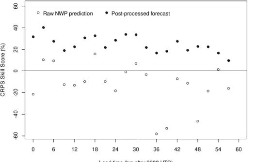
Figure 4 presents the CRPS skill scores of the raw NWP predictions and post pro-10
cessed rainfall forecasts for individual periods. The raw NWP predictions have negative skill for some individual periods, suggesting that it would be better to use a climatology forecast. However, post processing produces rainfall forecasts with positive skill for all lead times out to 57 h. Forecast skill is highest for rainfall predictions for the 3–6 h lead time and displays a gradual decline with increasing lead time. Post processing results 15
in marked improvements in skill over the raw NWP predictions, with the skill of the post processed forecast being on average 37 % higher than the raw NWP predictions.
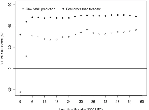
The skill of post processed forecasts of cumulative rainfall totals (Fig. 5), increases for the first three lead times and then remains relatively stable at a CRPS skill score of approximately 50 % out to 57 h. The raw NWP rainfall predictions display similar 20
HESSD
10, 6765–6806, 2013Post processing rainfall forecasts
D. E. Robertson et al.
Title Page
Abstract Introduction
Conclusions References
Tables Figures
◭ ◮
◭ ◮
Back Close
Full Screen / Esc
Printer-friendly Version Interactive Discussion
Discussion
P
a
per
|
Dis
cussion
P
a
per
|
Discussion
P
a
per
|
Discussio
n
P
a
per
|
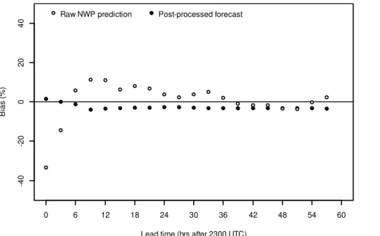
4.2.2 Forecast bias
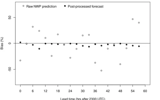
Figure 6 presents the bias in the raw NWP rainfall predictions and post processed fore-casts as a function of lead time. The post processed forefore-casts display little forecast bias at any lead time. Bias in the raw NWP rainfall predictions tends to be cyclical and can be as great as 50 % of the observed mean. The cyclic nature of biases in the raw 5
NWP rainfall predictions is likely the product of the limited ability of NWP models to describe the diurnal cycle. Post processing methods can overcome this limitation, pro-vided that they are developed in a manner that allows for diurnal variations in forecast performance, as done here.
Correction of the forecast bias will be the greatest contribution to improvements in 10
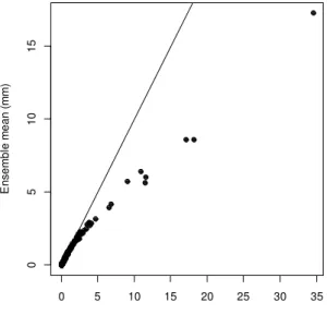
forecast skill. Figure 6 displays the correction to the mean bias, however bias correc-tion using the BJP modelling approach is more sophisticated than just correcting the mean bias. Using different marginal distributions, and particularly transformations, for the raw NWP rainfall predictions and observed data allows for a non-linear bias correc-tion (Fig. 7). This results in improvements in forecast skill that are greater than those 15
that would be achieved by just correcting the mean bias.
As expected from the previous analysis, biases in the post processed cumulative rainfall ensembles are minimal throughout the entire forecast period (Fig. 8). The biases for the raw NWP predictions decrease for lead times up to 9 h and then are relatively stable near zero. However, the magnitude of biases in the post processed ensemble 20
forecasts is nearly always smaller than the raw forecasts.
4.2.3 Forecast discrimination
Forecast discrimination is assessed using plots of the relative operating characteristic (ROC). The ability of the post processed forecasts to discriminate between events and non events varies with lead time and the event being considered (Fig. 9). At shorter 25
HESSD
10, 6765–6806, 2013Post processing rainfall forecasts
D. E. Robertson et al.
Title Page
Abstract Introduction
Conclusions References
Tables Figures
◭ ◮
◭ ◮
Back Close
Full Screen / Esc
Printer-friendly Version Interactive Discussion
Discussion
P
a
per
|
Dis
cussion
P
a
per
|
Discussion
P
a
per
|
Discussio
n
P
a
per
This suggests that forecasts for shorter lead times have a greater ability to discriminate between events and non-events than forecasts for longer lead times. The contrast in forecast discrimination with lead time is stronger for the high rainfall events (precipita-tion>5 mm) than for the events where rainfall is less than the event of rainfall less than 0.2 mm. This suggests that as lead time increases the post processed forecasts begin 5
to look more like a climatology forecast, with a decreasing probability of high rainfall. However, the ROC curves do not approach the diagonal line at any lead time, which suggests the post processed forecasts are always skilful. This is supported by the skill scores presented earlier.
The ROC curves for cumulative forecast rainfall totals display significantly less 10
spread than the curves for individual forecast periods. For the event of rainfall less than 0.2 mm, the forecast discrimination is stronger for shorter lead times than for longer lead times. However, for the events of greater than 5 mm, there are no clear differences in forecast discrimination with lead time.
4.2.4 Reliability
15
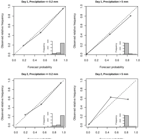
Figure 10 presents reliability diagrams for the probability of rainfall exceeding two thresholds for individual forecast periods pooled for lead times in day 1 and day 2. The reliability diagrams illustrate that the forecast probability of a rainfall event of less than 0.2 mm appears to be reliable, with the observed relative frequencies closely fol-lowing the line reflecting perfect reliability. The forecast probability of a rainfall event of 20
greater than 5 mm also appears to be reliable for day 1. For day 2 the forecast probabil-ity of a rainfall event of greater than 5 mm appears to be unreliable. However, very few forecasts have a probability of rainfall exceeding 5 mm that falls into the upper two bins of this diagram, and therefore, there is considerable sampling uncertainty associated with the observed frequencies.
25
HESSD
10, 6765–6806, 2013Post processing rainfall forecasts
D. E. Robertson et al.
Title Page
Abstract Introduction
Conclusions References
Tables Figures
◭ ◮
◭ ◮
Back Close
Full Screen / Esc
Printer-friendly Version Interactive Discussion
Discussion
P
a
per
|
Dis
cussion
P
a
per
|
Discussion
P
a
per
|
Discussio
n
P
a
per
|
of 24 h forecast rainfall totals exceeding than 5 mm, small deviations from the diagonal line occur for both day 1 and day 2 for the upper two bins. The number of samples in both of these bins is small and therefore subject to considerable sample variability. Overall, the forecasts of 24 h rainfall totals appear to be reliable.
The probabilistic forecasts of 24 h rainfall totals are produced by summing individual 5
ensemble members. These forecasts will only be reliable if the forecasts for individ-ual periods are reliable and the ensemble members have the appropriate space–time correlation structures. The space–time correlations in the ensemble members were in-troduced using the Schaake Shuffle. Here we have demonstrated that the probability distributions of forecasts for both individual periods and cumulative totals are reliable 10
and therefore the space–time correlations introduced by the Schaake Shuffle are ap-propriate.
5 Discussion
High quality forecasts of sub-daily rainfall are critical for forecasting streamflows, par-ticularly floods, in small and rapidly responding catchments. The marginal distributions 15
of sub-daily raw NWP rainfall predictions differ from those of the observations and therefore post processing is necessary. Observed rainfall displays a diurnal cycle, with maximum mean rainfall occurring between 3 and 9 p.m. in the afternoon, while the raw NWP predictions display little diurnal cycle. Poorly representing the timing and magni-tude of the diurnal cycles, particularly in precipitation, is a known problem with many 20
NWP models and is commonly related to the representation and parameterisation of convective processes (Evans and Westra, 2012; Dai and Trenberth, 2004). Therefore, it may be more appropriate to condition the post processing of NWP rainfall predictions on the type of rainfall rather than lead time. However, previous analysis found that er-rors in NWP rainfall predictions could not be predicted by synoptic or rainfall types for 25
HESSD
10, 6765–6806, 2013Post processing rainfall forecasts
D. E. Robertson et al.
Title Page
Abstract Introduction
Conclusions References
Tables Figures
◭ ◮
◭ ◮
Back Close
Full Screen / Esc
Printer-friendly Version Interactive Discussion
Discussion
P
a
per
|
Dis
cussion
P
a
per
|
Discussion
P
a
per
|
Discussio
n
P
a
per
One of the major challenges for developing and evaluating short term streamflow forecasting systems, and particularly post processing methods for rainfall predictions, in Australia is the limited availability of retrospective NWP predictions from the ACCESS suite of models. The lack of retrospective NWP predictions imposes some limitations on this study and the conclusions that can be drawn. Significant streamflow events, 5
including floods, result from significant rainfall events and therefore the ability to fore-cast significant rainfall events is critical. Few large, flood causing, rainfall events exist in the record of ACCESS predictions used in this study. Post processing methods that use parametric modelling, such as the one used in this study, can be used to extrap-olate relationships beyond the range of data used to fit the model and produce post 10
forecasts for rare events. However, the quality of these extrapolated forecasts cannot be comprehensively assessed. The reliability diagram for the probability of precipita-tion exceeding 5 mm for day two forecasts provides an example of this problem where the number of samples in the high forecast probability bins is very small and therefore no conclusive statement about the reliability of these forecasts can be made. In the 15
extreme case, such as in arid zones, it is possible that during the period of available retrospective NWP predictions no rainfall is observed or predicted for some forecast periods. This has the potential to prevent the establishment of a model and as a result post processing of NWP rainfall predictions may not be possible. Therefore, forecasts of extreme rainfall events need to be used with caution and methods need to be further 20
developed to handle situations where there are insufficient non-zero rainfall observa-tions and predicobserva-tions to establish a post processing model.
The post processing approach described in this paper models only the concurrent relationship between raw NWP predicted and observed rainfall to produce a rainfall forecast. It assumes that the temporal correlation in mean rainfall at different time pe-25
HESSD
10, 6765–6806, 2013Post processing rainfall forecasts
D. E. Robertson et al.
Title Page
Abstract Introduction
Conclusions References
Tables Figures
◭ ◮
◭ ◮
Back Close
Full Screen / Esc
Printer-friendly Version Interactive Discussion
Discussion
P
a
per
|
Dis
cussion
P
a
per
|
Discussion
P
a
per
|
Discussio
n
P
a
per
|
accommodate both these possibilities in a post processing method requires a more so-phisticated model where multiple forecast periods are included in a single model. The simplified BJP modelling approach used here can potentially be adapted to produce forecasts for multiple periods from a single model. However, it would require strong parameterisation of the correlation matrix to limit the risk of over fitting. Such an ap-5
proach is attractive as it would remove the need to use the Schaake shuffle to cre-ate ensembles from separcre-ately post processed probability distributions, as the spatial and temporal correlations would be explicitly modelled. Stronger assumptions about all model parameters may also be able to deal with situations where little or no rainfall is observed or predicted for some forecast periods.
10
In this study, the post processing method has only been applied to a catchment in the temperate zone of southern Australia. In this catchment, rainfall is predominantly produced by large scale synoptic systems moving across the catchment. Large scale synoptic systems are better predicted by NWP models because they tend to evolve relatively slowly and occur on spatial scales that are resolved by the models (Roux 15
and Seed, 2011; Roux et al., 2012). NWP models tend not to predict rainfall from convective systems well because these processes evolve rapidly and commonly occur on spatial scales finer than those resolved by the model. In areas where substantial rainfall is produced by convective systems, the raw NWP rainfall predictions may not be sufficiently correlated with rain gauge observations to produce skilful rainfall forecasts 20
using the method described in this paper. Further work is proposed to assess the efficacy of the post processing method for catchments experiencing a range of climatic conditions in Australia.
The motivation for post processing NWP rainfall predictions is to produce bias free ensemble rainfall forecasts that can be used for ensemble streamflow forecasting. Us-25
HESSD
10, 6765–6806, 2013Post processing rainfall forecasts
D. E. Robertson et al.
Title Page
Abstract Introduction
Conclusions References
Tables Figures
◭ ◮
◭ ◮
Back Close
Full Screen / Esc
Printer-friendly Version Interactive Discussion
Discussion
P
a
per
|
Dis
cussion
P
a
per
|
Discussion
P
a
per
|
Discussio
n
P
a
per
of future investigations. Part of these investigations will include examining the temporal resolution at which post processed rainfall forecasts are most skilful and which lead to the most skilful streamflow forecasts.
6 Conclusions
Sub-daily ensemble rainfall forecasts that are bias free and reliably quantify forecast 5
uncertainty are critical for flood and short term ensemble streamflow forecasting. The raw output from numerical weather prediction models typically does not provide rainfall forecasts with these properties and therefore some form of post processing is required. In this paper we describe a new approach to generate ensemble rainfall forecasts by post processing raw NWP rainfall predictions. The approach uses a simplified version 10
of the Bayesian joint probability modelling approach, which was designed for seasonal streamflow forecasting, to produce forecast probability distributions for individual loca-tions and forecast periods. Ensemble forecasts with appropriate spatial and temporal correlations are then generated by linking samples from the forecast probability distri-butions using the Schaake shuffle.
15
We apply the approach to post process rainfall predictions from the ACCESS-R nu-merical weather prediction model at rain gauge locations in the Ovens catchment in southern Australia. We demonstrate that the assumed log-sinh transformed multivari-ate normal distribution is approprimultivari-ate for modelling the joint distribution of NWP pre-dicted and observed rainfall. The method is shown to produce ensemble forecasts that 20
are more skilful than the raw NWP predictions both for individual forecast periods and for cumulative totals throughout the forecast periods. Skill increases result from the correction of not only the mean bias, but also biases conditional on the magnitude of the NWP rainfall prediction. The post processed forecast ensembles are demonstrated to successfully discriminate between events and non-events for both small and large 25
HESSD
10, 6765–6806, 2013Post processing rainfall forecasts
D. E. Robertson et al.
Title Page
Abstract Introduction
Conclusions References
Tables Figures
◭ ◮
◭ ◮
Back Close
Full Screen / Esc
Printer-friendly Version Interactive Discussion
Discussion
P
a
per
|
Dis
cussion
P
a
per
|
Discussion
P
a
per
|
Discussio
n
P
a
per
|
This study has assessed the post processing approach for conditions where rainfall is principally due to large scale synoptic systems. Further work is proposed to assess the efficacy of the post processing method for catchments experiencing a range of climatic conditions in Australia, particularly in areas where significant rainfall is the result of convective processes. Future investigations will also assess the benefits of 5
using post processed rainfall forecasts for flood and short term streamflow forecasting and examine the temporal resolution at which rainfall post processing is most effective.
Appendix A
Reparameterisation of model parameters
To ease parameter inference, the all the parameters of the transformed multivariate 10
model are reparameterised. The parametersµandσ are strongly related to the trans-formation parameters. These parameters are reparameterised tomand s, which are first order Taylor series approximations ofµandσ in the untransformed space.
µi = 1
bi ln (sinh (αi+βimi))
σi = 1
tanh (αi+βimi)
si
15
wherei=1, 2,. . .,d.
Further reparameterisation of m and s to m∗ and s∗, allows for parameter estima-tion on the entire real space and an approximately linear dependence between the estimated parameters.
20
m∗i =ln
mi+αi
βi
HESSD
10, 6765–6806, 2013Post processing rainfall forecasts
D. E. Robertson et al.
Title Page
Abstract Introduction
Conclusions References
Tables Figures
◭ ◮
◭ ◮
Back Close
Full Screen / Esc
Printer-friendly Version Interactive Discussion
Discussion
P
a
per
|
Dis
cussion
P
a
per
|
Discussion
P
a
per
|
Discussio
n
P
a
per
Logarithms are taken of the two transformation parameters (α andβ). The correlation coefficient matrix R is reparameterised to Φ using an inverse hyperbolic tangent or
Fisher Z-transformation (Wang et al., 2009), to give
Φ=
∞ φ12 · · · φ1d φ21 ∞ · · · φ2d
..
. ... . .. ... φd1φd2 · · · ∞
where 5
φi j =tanh−1(ri j).
The collection of parameters used in inference is
θ={ln (α) , ln (β) ,m∗,s∗,Φ}.
Appendix B
Posterior parameter distribution
10
According to Bayes’ theorem, the posterior distribution of model parameters is
p θ|YOBS
∝p(θ)p YOBS|θ=p(θ) n Y
t=1
pytOBS|θ
wherep(θ) is the prior distribution representing information available about parameters before the use of historical data andp YOBS|θ
HESSD
10, 6765–6806, 2013Post processing rainfall forecasts
D. E. Robertson et al.
Title Page
Abstract Introduction
Conclusions References
Tables Figures
◭ ◮
◭ ◮
Back Close
Full Screen / Esc
Printer-friendly Version Interactive Discussion
Discussion
P
a
per
|
Dis
cussion
P
a
per
|
Discussion
P
a
per
|
Discussio
n
P
a
per
|
ytOBS is the observed predictor and predictand data for event t (t=1, 2,. . .,n), given the model and its parameter set.
The BJP modelling approach treats occurrences of zero values as censored data, where data are known to be less than or equal a censoring value with an unknown precise value. Formulation of the likelihood functionp YOBS|θ
allows for general cen-5
soring thresholds (yc). To evaluate the likelihood function, the vectory is rearranged into two subvectors
y=
y(a)
y(b)
where y(a) consists of variables whose values are above their respective censor thresholds yc(a) and precisely known, and y(b) consists of variables whose values 10
are only known to be equal to or below their respective censor thresholdsyc(b). The vector of transformed variables is organised as
z=
z(a)
z(b)
.
The likelihood function is then given by
p y|θ=
p y(a) ,y(b)≤yc(b)|θ=
p y(a)|θ
×p y(b)≤yc(b)|y(a) ,θ 15
where
p y(a)|θ=
Jz(a)→y(a)p z(a)|θ=
da
Y
i=1
dz i dyi
p z(a)|θ
p y(b)≤yc(b)|y(a) ,θ=
p z(b)≤zc(b)|z(a) ,θ=
zc(b)
Z
−∞
p z(b)|z(a) ,θ
HESSD
10, 6765–6806, 2013Post processing rainfall forecasts
D. E. Robertson et al.
Title Page
Abstract Introduction
Conclusions References
Tables Figures
◭ ◮
◭ ◮
Back Close
Full Screen / Esc
Printer-friendly Version Interactive Discussion
Discussion
P
a
per
|
Dis
cussion
P
a
per
|
Discussion
P
a
per
|
Discussio
n
P
a
per
wherezc(b) is the transformed values of the censor threshold corresponding toyc(b). The Jacobian determinantJz(a)→y(a) of the transformation fromz(a) toy(a) is dzi
dyi
= 1
tanh (αi+βiyi) .
Appendix C
Prior distribution of parameters
5
The prior distribution for the model parameters is specified as
p(θ)=
d Y
i=1
p(lnαi)p(lnβi)p m∗i,si∗
p(Φ).
A uniform prior is specified for both of the transformation parameters, however because these parameters are not directly estimated it is necessary to apply the Jacobian of the reparameterisation to the uniform prior
10
p(lnα)=J
α→lnαp(α) ,
where the Jacobian determinant of the reparameterisation Jα→lnα
is given by
Jα→lnα= dα
d (lnα) =α, and
p(α)∝1.
15
Similarly,
HESSD
10, 6765–6806, 2013Post processing rainfall forecasts
D. E. Robertson et al.
Title Page
Abstract Introduction
Conclusions References
Tables Figures
◭ ◮
◭ ◮
Back Close
Full Screen / Esc
Printer-friendly Version Interactive Discussion
Discussion
P
a
per
|
Dis
cussion
P
a
per
|
Discussion
P
a
per
|
Discussio
n
P
a
per
|
where the Jacobian determinant of the reparameterisation Jβ→lnβ
is given by
Jβ→lnβ= dβ
d (lnβ) =β,
and
p(β)∝1.
A more elaborate prior for the pair of m∗,s∗is used to deal with the reparameterisa-5
tions, giving
p(m∗,s∗)=Jµ,σ2
→m,s2Js2→s∗Jm→m∗p
µ,σ2,
where the Jacobian determinant of the transformation Jµ,σ2→m,s2 from
µ,σ2 to
m,s2is given by
Jµ,σ2→m,s2 =
∂µ ∂m
∂µ ∂s2 ∂σ2
∂m ∂σ2 ∂s2
=
1
tanh (αi+βimi) 3
, 10
the Jacobian determinant of the reparameterisation Js2→s∗
froms2tos∗is given by
Js2→s∗=
d s2
d s∗ =s
2,
the Jacobian determinant of the reparameterisation(Jm→m∗) from m tom∗ is given by
Jm→m∗=
dm
dm∗ =m+ α
HESSD
10, 6765–6806, 2013Post processing rainfall forecasts
D. E. Robertson et al.
Title Page
Abstract Introduction
Conclusions References
Tables Figures
◭ ◮
◭ ◮
Back Close
Full Screen / Esc
Printer-friendly Version Interactive Discussion
Discussion
P
a
per
|
Dis
cussion
P
a
per
|
Discussion
P
a
per
|
Discussio
n
P
a
per
andpµ,σ2takes the simplest form of priors commonly used for normal distribution mean and variance (Wang and Robertson, 2011; Gelman et al., 1995)
pµ,σ2∝ 1
σ2.
The prior for the reparameterised correlation coefficient is related to the prior for the original correlation coefficient by
5
p(Φ)=JR→Φp(R)=
d−1
Y
i=1
d Y
j=i+1
dri j dϕi j
p(R)
whereJR→Φis the Jacobian determinant for the transform fromRtoΦ, and
dri j dϕi j
=
cosh ϕi j−2 .
A marginally uniform prior is used for the correlation matrix (Barnard et al., 2000; Wang et al., 2009)
10
p(R)∝ |R|
d(d−1)
2 −1 d Y
i=1
|Ri i| !
−(d−1) 2
whereRi i is theith principal submatrix ofR.
Acknowledgements. This research has been supported by the Water Information Research and Development Alliance between the Australian Bureau of Meteorology and CSIRO Water for a Healthy Country Flagship and the CSIRO OCE Science Leadership Scheme. We would
15
HESSD
10, 6765–6806, 2013Post processing rainfall forecasts
D. E. Robertson et al.
Title Page
Abstract Introduction
Conclusions References
Tables Figures
◭ ◮
◭ ◮
Back Close
Full Screen / Esc
Printer-friendly Version Interactive Discussion
Discussion
P
a
per
|
Dis
cussion
P
a
per
|
Discussion
P
a
per
|
Discussio
n
P
a
per
|
References
Australian Bureau of Meteorology: Operational Implementation of the ACCESS Numerical Weather Prediction Systems, Australian Bureau of Meteorolgy, Melbourne, 34 pp., 2010. Barnard, J., McCulloch, R., and Meng, X. L.: Modeling covariance matrices in terms of standard
deviations and correlations, with application to shrinkage, Stat. Sin., 10, 1281–1311, 2000.
5
Bl ¨oschl, G.: Flood warning – on the value of local information, Int. J. River Basin Manage., 6, 41–50, doi:10.1080/15715124.2008.9635336, 2008.
Charles, A., Hendon, H. H., Wang, Q. J., Robertson, D. E., and Lim, E.-P.: Comparsion of Techniques for the Calibration of Coupled Model Forecasts of Murray Darling Basin Seasonal Mean Rainfall, The Centre of Australian Weather and Climate Research, Melbourne, 38 pp.,
10
2011.
Clark, A. J., Kain, J. S., Stensrud, D. J., Xue, M., Kong, F., Coniglio, M. C., Thomas, K. W., Wang, Y., Brewster, K., Gao, J., Wang, X., Weiss, S. J., and Du, J.: Probabilistic precipita-tion forecast skill as a funcprecipita-tion of ensemble size and spatial scale in a convecprecipita-tion-allowing ensemble, Mon. Weather Rev., 139, 1410–1418, doi:10.1175/2010mwr3624.1, 2011.
15
Clark, M., Gangopadhyay, S., Hay, L., Rajagopalan, B., and Wilby, R.: The Schaake shuffle: a method for reconstructing space–time variability in forecasted precip-itation and temperature fields, J. Hydrometeorol., 5, 243–262, doi:10.1175/1525-7541(2004)005<0243:tssamf>2.0.co;2, 2004.
Dai, A. and Trenberth, K. E.: The diurnal cycle and its depiction in the community climate system
20
model, J. Climate, 17, 930–951, doi:10.1175/1520-0442(2004)017<0930:tdcaid>2.0.co;2, 2004.
Duan, Q., Sorooshian, S., and Gupta, V. K.: Optimal use of the SCE-UA global optimization method for calibrating watershed models, J. Hydrol., 158, 265–284, 1994.
Ebert, E. E.: Ability of a poor man’s ensemble to predict the probability and
dis-25
tribution of precipitation, Mon. Weather Rev., 129, 2461–2480, doi:10.1175/1520-0493(2001)129<2461:aoapms>2.0.co;2, 2001.
Evans, J. and Westra, S.: Investigating the mechanisms of diurnal rainfall variability using a re-gional climate model, J. Climate, 25, 7232–7247, doi:10.1175/jcli-d-11-00616.1, 2012. Gelman, A., Carlin, J. B., Stern, H. S., and Rubin, D. B.: Bayesian Data Analysis, in: Texts
30
HESSD
10, 6765–6806, 2013Post processing rainfall forecasts
D. E. Robertson et al.
Title Page
Abstract Introduction
Conclusions References
Tables Figures
◭ ◮
◭ ◮
Back Close
Full Screen / Esc
Printer-friendly Version Interactive Discussion
Discussion
P
a
per
|
Dis
cussion
P
a
per
|
Discussion
P
a
per
|
Discussio
n
P
a
per
George, B. A., Adams, R., Ryu, D., Western, A. W., Simon, P., and Nawarathna, B.: An Assess-ment of Potential Operational Benefits of Short-term Stream Flow Forecasting in the Broken Catchment, Victoria, Proceedings of the 34th IAHR World Congress, Brisbane, Australia, 2011.
Glahn, H. R. and Lowry, D. A.: The use of Model Output Statistics (MOS) in
ob-5
jective weather forecasting, J. Appl. Meteorol., 11, 1203–1211, doi:10.1175/1520-0450(1972)011<1203:tuomos>2.0.co;2, 1972.
Hamill, T. M. and Colucci, S. J.: Verification of Eta-RSM short-range ensemble forecasts, Mon. Weather Rev., 125, 1312–1327, doi:10.1175/1520-0493(1997)125<1312:voersr>2.0.co;2, 1997.
10
Hamill, T. M., Whitaker, J. S., and Wei, X.: Ensemble reforecasting: improving medium-range forecast skill using retrospective forecasts, Mon. Weather Rev., 132, 1434–1447, doi:10.1175/1520-0493(2004)132<1434:erimfs>2.0.co;2, 2004.
Hersbach, H.: Decomposition of the continuous ranked probability score for ensemble predic-tion systems, Weather Forecast., 15, 559–570, 2000.
15
Jolliffe, I. T. and Stephenson, D. B.: Forecast Verification: a Practitioner’s Guide in Atmospheric Science, J. Wiley, Chichester, 240 pp., 2003.
Kleiber, W., Raftery, A. E., and Gneiting, T.: Geostatistical Model Averaging for Locally Cali-brated Probabilistic Quantitative Precipitation Forecasting, Department of Statistics, Univer-sity of Washington, Seattle, WA, USA, 2010.
20
Penning-Rowsell, E. C., Tunstall, S. M., Tapsell, S. M., and Parker, D. J.: The benefits of flood warnings: real but elusive, and politically significant, Water Environ. J., 14, 7–14, doi:10.1111/j.1747-6593.2000.tb00219.x, 2000.
Robertson, D. E. and Wang, Q. J.: A Bayesian approach to predictor selection for seasonal streamflow forecasting, J. Hydrometeorol., 13, 155–171, 2012.
25
Roulin, E.: Skill and relative economic value of medium-range hydrological ensemble predic-tions, Hydrol. Earth Syst. Sci., 11, 725–737, doi:10.5194/hess-11-725-2007, 2007.
Roux, B. and Seed, A. W.: Assessment of the Accuracy of the NWP Forecasts for Significant Rainfall Events at the Scales Needed for Hydrological Prediction, Bureau of Meteorology, Melbourne, 2011.
30


![Fig. 3. Observed (red dots) and modelled median (vertical lines, representing [0.05, 095] un- un-certainty range) correlation coefficients between NWP forecast and observed precipitation for post processing models covering lead times from 0 to 57 h at site](https://thumb-eu.123doks.com/thumbv2/123dok_br/16364388.190512/34.918.208.505.141.426/observed-vertical-representing-certainty-correlation-coefficients-precipitation-processing.webp)