The wave climate and its seasonal variability in the northeastern
Baltic Sea
Andrus Räämet
a,band Tarmo Soomere
ba
Department of Mechanics, Faculty of Civil Engineering, Tallinn University of Technology, Ehitajate tee 5, 19086 Tallinn, Estonia; [email protected]
b
Institute of Cybernetics at Tallinn University of Technology, Akadeemia tee 21, 12618 Tallinn, Estonia; [email protected]
Received 8 September 2009, accepted 5 January 2010
Abstract. The basic features of wave properties in the Baltic Sea and their seasonal variations are estimated by the use of a high-resolution version (3 miles) of the wave model, WAM, driven by adjusted geostrophic winds for 1970–2007 under ice-free conditions. The model qualitatively reproduces the time series of the sea state and adequately replicates the seasonal patterns of wave intensity and the probability distribution functions for different wave heights in both offshore and coastal regions of the northern Baltic Proper and the Gulf of Finland. The areas of the largest overall wave activity are located in the eastern parts of the Bothnian Sea and northern Baltic Proper, south of Gotland, and in the Arkona Basin. The windiest season (September–February) and the time with the largest measured or modelled wave activity (October–March) occur with a time lag of 0.5–2 months.
Key words: environmental science, wave climate, wave modelling, wind climate, geostrophic wind.
INTRODUCTION
The combination of significant wind anisotropy and seasonal variation in the wind speed gives rise to high anisotropy and large spatio-temporal variations in the Baltic Sea wave fields (Jönsson et al. 2002; Soomere 2003; Broman et al. 2006; Kelpšaite et al. 2008). The areas with the largest average wave intensity are apparently formed under relatively high mean wind speeds and large fetch in the southern and (north)eastern regions of the Baltic Sea (Jönsson et al. 2002). The monthly maximum wave heights occur in the northern-most and southernnorthern-most coastal regions of this water body. Waves may be extremely high also offshore the coasts of Latvia and Saaremaa (Jönsson et al. 2002; Soomere et al. 2008). Several related characteristics such as hydrodynamic bottom stress and resuspension patterns are strongly correlated with the features of the wave climate listed above (Elken et al. 2002; Jönsson et al. 2005). Although a few numerical wave modelling studies have been carried out in the recent past (Cieślikiewicz & Paplińska-Swerpel 2008; Kriezi & Broman 2008), there is no adequate assessment of the spatial variability of the wind-wave intensity for the Baltic Sea in the international scientific literature. Using the global wave data set KNMI/ERA-40Wave Atlas (09.1957–08.2002, Sterl & Caires 2005), a reliable wave climatology can be produced for open ocean conditions but its spatial
resolution (1.5° × 1.5°) is too sparse for the Baltic Sea conditions. This paper attempts to fill this gap based on numerical simulations over 38 years.
Recent studies have revealed several intriguing patterns of the long-term behaviour of the Baltic Sea wave fields. The most important change is the observed rapid increase in the annual mean wave height in the northern Baltic Proper (NBP) from the mid-1980s until the mid-1990s and a rapid decrease since then (Broman et al. 2006; Soomere & Zaitseva 2007). There is some uncertainty about the significance of other factors (such as instrument failure, observers’ error or noise in the data; Broman et al. 2006; Soomere & Zaitseva 2007) affecting the observed and measured changes. As the recorded changes occurred simultaneously, and with a similar relative range at both eastern and western coasts of the NBP, they appear to show large-scale decadal variations in the wave properties. Interestingly, similar decadal variations were much weaker in semi-enclosed bays of the northern coast of Estonia and on the Lithuanian coast (Kelpšaite et al. 2008, 2009).
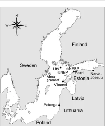
Fig. 1. Location of coastal observation sites (filled circles) and calculation points of offshore wave properties (crossed circles). NBP, northern Baltic Proper; NEBP, northeastern Baltic Proper.
against a five-month data set and then forced with high- quality wind data from Vilsandi Island for 1966–2006 (Räämet et al. 2009; Suursaar & Kullas 2009; Zaitseva-Pärnaste et al. 2009). Although the annual mean wind speed decreased by more than 10% over this period (Kull 2005), only marginal changes were recorded in the annual mean wave height (Suursaar & Kullas 2009).
The discrepancy between the match of the temporal pattern of the wind speed and wave heights may have its origin, for example, in gradual changes in the pre-dominant wind direction, intensity, trajectory, or in the persistence of storms. During the period in question, the frequency of southwestern winds has increased almost twofold at the expense of eastern and southern winds (Kull 2005). This change may cause an increase in wave heights in the entire NBP (Broman et al. 2006; Soomere & Zaitseva 2007) but has almost no impact on wave fields in fetch-limited conditions in the bays of northern Estonia and in the southeastern Baltic Sea (Kelpšaite et al. 2008, 2009).
Part of the mismatch can be explained by different trends in the wind speed in different months. For example, there has been a clear decrease in the wind speed in summer but a pronounced increase in December and January (Kull 2005). These changes are not easy to identify, because seasonal variations (for example, the
monthly mean) in the wind speed match well with similar variations in wave intensity. This match is evident in both the observed and modelled wave data (Jönsson et al. 2002; Kahma et al. 2003; Broman et al. 2006; Soomere & Zaitseva 2007; Räämet et al. 2009; Zaitseva-Pärnaste et al. 2009). We make an attempt to shed light on this problem by analysing the relationship between wind and wave properties in different months. The key idea behind doing this is the nonlinear dependence of wave heights on the wind speed. Generally, an increase in an already high wind speed results in a larger increase in wave heights than the same increase for a low wind speed (Komen et al. 1994). Therefore, a substantial increase in wave heights because of a growth in the wind speed in a few windy (autumn and winter) months may dominate over the similar decrease in low wave heights in calm (spring and summer) months.
The properties of wave fields in the Baltic Sea essentially depend on the relationship between the area of high winds, the wind direction, and the geometry of the water body. This dependence is only partially accounted for in one-point models. In contrast to most of the simulations performed so far, our high-resolution numerical hindcast of spatio-temporal patterns of wave fields covers the entire Baltic Sea for 38 years (1970– 2007). It allows the identification of the basic properties of both seasonal and long-term variations in the wave fields in different parts of the Baltic Sea.
The wave model is forced by the first approximation of the spatio-temporal patterns of wind fields derived from geostrophic winds. The use of modelled winds makes the results virtually independent of local distortions of winds at ground measurement sites which are frequently quite large at coastal observation sites in the Baltic Sea (Keevallik 2003; Soomere & Keevallik 2003). The choice of forcing was based on pilot calculations using several publicly available wind databases, such as the Operational Mesoscale Analysis System (MESAN; Häggmark et al. 2000). The bias and root-mean-square deviation between the observed (or measured) and numerically simulated data was generally acceptable and frequently the best for properly adjusted geostrophic winds (Räämet et al. 2009) which thus can be considered as the best compromise between robustness and low spatial resolution of the geostrophic wind data, and the potential distortions of the local wind field in higher-resolution local atmospheric models (Ansper & Fortelius 2003; Keevallik et al. 2010). Also, the principal changes in the local climate that are driven by changes in large-scale circulation patterns should become evident in the properties of geostrophic winds.
influencing wave fields in the Baltic Sea. The ice cover not only reshapes the area of wave generation (fetch length, thereby affecting waves even far down-wind from the ice region) but also affects atmospheric conditions so that the wind speed over a frozen sea may be larger than over rough wind-generated seas.
The presentation starts with the description of the setup of the wave model and forcing conditions. Next, the basic statistical features of the measured, observed, and numerically simulated wave properties are discussed in terms of time series and monthly means of the significant wave height HS and the seasonal variability of the wave fields is analysed. Finally, long-term changes in the seasonal properties of wave fields are compared against similar properties of high-quality marine winds at Utö Island.
WAM MODEL AND WIND FORCING FOR THE BALTIC SEA
Wave properties over the entire Baltic Sea were computed by the use of the third-generation wave model, WAM cycle 4 (Komen et al. 1994), over 38 years for 1970–2007. The bathymetry was based on data prepared by Seifert et al. (2001) (http://www.io-warnemuende.de/topography-of-the-baltic-sea.html) and has been adjusted as described in Soomere (2001). The calculation was undertaken over a regular rectangular grid with a resolution of about 3 × 3 nautical miles. The grid increment is 3′ for latitude and 6′ for longitude. The entire grid contains 239 × 208 points (11 545 seapoints) and extends from 09°36′E to 30°18′E and from 53°57′N to 65°51′N. This resolution is somewhat finer than that used in other calculations in the recent past (Jönsson et al. 2002, 2005; Cieślikiewicz & Paplińska-Swerpel 2008; Kriezi & Broman 2008).
The wave properties in the Baltic Sea can be modelled with the use of local models, because the waves from the rest of the world ocean practically do not affect this water body (Soomere 2001, 2008). The model was run uncoupled from the North Sea wave fields on a grid that was truncated in the narrowest parts of the Danish Straits. The hindcast was performed in shallow-water mode with depth refraction (but without depth-induced breaking) in order to match realistic wave propagation patterns over the highly variable bathymetry of the relatively shallow Baltic Sea.
At each seapoint 1008 components of the two-dimensional spectrum were computed. The spectrum contained 24 equally spaced directions (with the angular resolution of 15°) starting from the direction of 7.5° and counted counterclockwise from the direction to the
north. The energy of wave components with frequencies ranging from 0.042 Hz (23.9 s) to about 2 Hz (0.5 s) was approximated using 42 frequencies with an increment of 1.1. The extended frequency range up to 2 Hz was used to ensure realistic wave growth in low wind conditions after periods of calm. Such situations are frequent in the Baltic Sea where the standard con-figuration of the WAM model (that ignores waves with periods below 2 s) does not ensure the realistic growth of relatively short waves (Soomere 2005). The propagation and source time step were both set to 180 s to ensure numerical stability of the integration scheme. The wave properties were recorded hourly for the entire period of calculations.
A critical issue in wave modelling is the choice of the wind forcing for which no universal solution exists (Signell et al. 2005; Bertotti & Cavaleri 2009). The wave model was forced with wind data constructed on the basis of geostrophic winds provided by the Swedish Meteorological and Hydrological Institute (SMHI). These data are mainly calculated from the spatial air pressure distribution and, therefore, are free of local disturbances to the air flow by coastal topography and errors in ground wind speed measurements (Keevallik 2003; Soomere & Keevallik 2003). On the other hand, the use of these data smoothes out a large number of local variations in wind properties. As geostrophic winds represent global (in the scale of the Baltic Sea) wind patterns, the relevant wave properties reflect well the principal properties of wind patterns on the open sea, which are mostly responsible for the wave climatology.
PERFORMANCE OF THE MODEL
The wave model together with the described forcing reproduces adequately the time series of wave conditions in the NBP (Fig. 3). The simulations catch all important wave events and their duration in most cases. The maximum wave heights are somewhat overestimated for some storms and underestimated for other wind events. Such mismatches in time series of the measured and modelled wave properties are common in contemporary efforts to model wave conditions in the Baltic Sea (Tuomi et al. 1999; Jönsson et al. 2002; Lopatukhin et al. 2006; Cieślikiewicz & Paplińska-Swerpel 2008; Soomere
et al. 2008). In our simulations some deviations probably stem from the choice of the wind forcing that ignores local ageostrophic wind components. There is, however,
no large systematic bias of the results and the overall average of wave heights is also reproduced reasonably (Table 1, Fig. 4).
The model also represents well the overall average properties of wave conditions in those Estonian coastal waters that are open to the Baltic Proper (Räämet et al. 2009). The best match is obtained for long-term averages of wave fields (Table 1). Their comparison, however, is not straightforward because the periods only partially overlap, yet it indicates the utility of the modelling approach used. For example, the observed and modelled average wave heights at Vilsandi differ by less than 1 cm (equivalently, by less than 2%) over the period 1970– 2007 (Table 1). The match is of almost the same quality at Pakri for 1970–85 (Zaitseva-Pärnaste 2009), whereas the overall observed wave height in 1954–85 is very (a)
(b)
Fig. 3.Measured (thin line) and hindcast (bold line) significant wave heights at Almagrundet in December 1986. The bias and root-mean-square deviation (RMSD) between the modelled (average 1.34 m) and hindcast (1.52 m) data were 18.7 and 63.9 cm, respectively. Note that the bias and RSMD between the observed and modelled data were, respectively, 19 and 44 cm at Almagrundet in 1999 (Jönsson et al. 2002).
Table 1. Average observed or measured and hindcast wave properties at the measurement sites in the northern Baltic Proper and the Gulf of Finland (Broman et al. 2006; Zaitseva-Pärnaste 2009). For visual observation sites the average of daily mean values is presented (Soomere & Zaitseva 2007)
Average wave height, m Site Years
Observed or measured
Hindcast
1978–1995 0.876 0.714 Almagrundet
1993–2003 1.040 0.705
Vilsandi 1954–2008 1970–2007
0.575 0.560
– 0.563
Pakri 1954–1985 1970–1985
1970–2007
0.591 0.571 –
– 0.569 0.584
Narva-Jõesuu 1954–2008 1970–2007
0.390 0.368
– 0.466 ————————
– no data.
close to that calculated for 1970–2007 (Table 1). The model, therefore, reproduces well the long-term wave heights for the western and northwestern coasts of Estonia.
The results of numerical simulations deviate more from the observed data in relatively sheltered areas where the model tends to overestimate wave heights. At Narva-Jõesuu the modelled average wave height exceeds the observed value by more than 25% (Table 1). There are several reasons for such a deviation. A generic source of error is the insufficient spatial resolution of the wave
Fig. 4. Scatter plot of the measured and numerically simulated wave heights at Almagrundet in 1991. The brightness scale shows the number of wave conditions in pixels with dimensions of 0.05 m × 0.05 m. The overall bias is 21.1 cm (observed waves are generally higher) and the root-mean-square deviation is 54.1 cm.
model in coastal areas (cf. Räämet et al. 2009). The water depth is 3–4 m in the nearshore about 300 m from the coast where the wind wave properties are observed at Narva-Jõesuu. The centre of the closest model grid point, however, is located about 4 km from the site and corresponds to a depth of 7 m. As the waves are generally of moderate height and length at Narva-Jõesuu (see below), the effect of the depth-induced breaking on the observed wave properties is generally negligible at this site. The overestimation at Narva-Jõesuu may also be due to the joint effect of ignoring the ice cover and the difference between the observation site and the nearest grid point for which the wave properties are calculated.
Another criterion demonstrating the performance of the wave model is the match between the frequency of occurrence of different hindcast, observed, and measured wave conditions within a certain range, equivalently, between the relevant probability distribution functions (PDFs). The comparison below is performed only for wave heights, which are always recorded in wave measure-ments and observations. The results of such comparisons are usually expressed as bar charts of empirical PDFs. Although such charts are quite sensitive with respect to the thresholds used, they are generally as instructive as the comparisons of the time series for selected periods, average wave properties, or scatter plots discussed above.
At Almagrundet the model underestimates the frequency of almost calm conditions (HS<0.25 m),
largely overestimates waves with 0.25≤HS<0.75 m,
and underestimates the frequency of waves higher than 1 m, whereas the discrepancy is less for wave heights
S 2.5 m
H ≥ (Fig. 5). This pattern of mismatches is qualitatively similar to that obtained using the 1999 simulations discussed above, where the HYPAS model (Jönsson et al. 2002) overestimates waves with heights
S 0.4 m
H < and 0.8≤HS <1.4 m and underestimates
waves about 0.5 m high and all wave conditions with
S 1.6 m.
H ≥
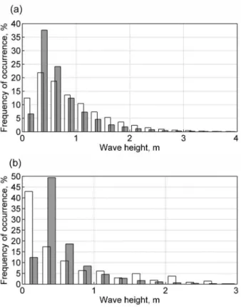
Fig. 5. Frequency of occurrence of wave heights: (a) at Almagrundet in 1978–95 (white bars: measurements, Broman et al. 2006; grey bars: WAM model); (b) at Vilsandi (white bars: observations 1954–2008, Zaitseva-Pärnaste 2009; grey bars: WAM model 1970–2007).
A large part of the difference between the modelled results and observations probably stems from the choice of the threshold at 0.25 m: the frequency of observed (36%) and modelled (44%) low wave conditions
S
(H <0.5 m) differ insignificantly. The same is true for the results of Jönsson et al. (2002). The largest relative difference occurs for waves higher than 1 m that seem to be systematically underestimated by the models at Almagrundet. As mentioned above, a large part of this difference may stem from measurement noise.
At Vilsandi the model also underestimates waves below 0.25 m and overestimates waves with
S
0.25≤H <0.5 m (Fig. 5). The overall characteristics of waves with a height below 0.5 m are again reasonably captured. While waves with heights around 1–1.5 m are sensibly reproduced, the frequency of even higher waves is underestimated. This pattern of mismatches becomes evident also in simulations with the use of a one-point model forced with Vilsandi winds (Suursaar & Kullas 2009) and may be an overall feature of wave properties in the coastal areas of Saaremaa.
A slightly different pattern of discrepancies becomes evident in the central part of the NBP and in the coastal area of Lithuania (Fig. 6). The model adequately captures
the frequency of calm conditions and reasonably hindcasts relatively high wind-generated seas. The frequency of the most typical wave conditions (0.25≤HS<0.75 m)
is, however, significantly overestimated by the model. Surprisingly, the model gives one of the best matches with observations at Pakri. As the measurements there ceased in 1985, wave properties from different time intervals are presented in Fig. 7. Only the frequency of 0.25–0.5 m high waves is overestimated by the model. The match is less satisfactory at Narva-Jõesuu where very low waves (HS<0.25 m) form almost half the
observed data but are not captured by the model. This feature is not unexpected at this site where the dominant winds are blowing off the land and low waves are frequently observed even under relatively high wind speeds. The same situation may also occur at times at Pakri where there is a relatively large deep sea area in the southern and southwestern directions.
Another reason for the frequent presence of low waves and the mismatch between the modelled and observed data is the sea-breeze that is very well developed in northeastern Estonia over the summer season and occasionally also in autumn (when it is driven by the
Fig. 7. Frequency of occurrence of wave heights: (a) at Pakri (white bars: observations 1954–85, Zaitseva-Pärnaste 2009; grey bars: WAM model 1970–2007); (b) at Narva-Jõesuu in 1970–2007 (white bars: observations, Zaitseva-Pärnaste 2009; grey bars: WAM model).
temperature difference between the cold land and the warm sea). As the wind turns over the day under sea-breeze conditions, the wave height is to some extent affected by this phenomenon that may locally create larger waves than weak geostrophic wind in remote sea areas. Also, ice conditions frequently impact the sea state at this site (Sooäär & Jaagus 2007). The match of the modelled and observed data for all waves with heights <0.5 m is, however, good, as it is for the distribution of higher waves.
The overall shape of the numerically simulated distributions of the occurrence of different wave heights varies in different places, mirroring the relative openness of the sea areas (Fig. 8). The smallest fraction of low waves occurs in the central NBP. Larger fractions are evident in coastal areas at Pakri and Vilsandi and the largest at Narva-Jõesuu. Conversely, the fraction of large waves is the highest on the open sea. A ‘threshold’ separating the different content of waves in these distributions is at the wave height of about 0.75 m, which roughly corresponds to the long-term mean wave height in open sea areas (Table 1).
The mismatch between the modelled and observed wave properties is the largest for low wave heights
S
(H <0.25 m). Accurate modelling and measurement of such waves is a challenge and the results are frequently very sensitive with respect to the particular procedure. Many of the mismatches probably stem from the inaccuracies of the wind data. For example, the HIRLAM (stands for High Resolution Limited Area Model) model, used as a first guess in the MESAN analyses, often underestimates the wind field (Jönsson 2005). The MESAN analyses also underestimate the winds (Häggmark et al. 2000). The adjusted geostrophic wind data lead to about the same accuracy of reproduction of the frequency of different wind conditions. Another intrinsic reason for the discrepancy between the observed
and hindcast wave data is that most of the observation points are located much closer to the coast than the relevant centres of the grid cells. Therefore it is safe to say that the model in use satisfactorily reproduces both the basic long-term properties of wave fields and also the empirical distributions of different wave heights.
WAVE CLIMATE AND ITS SEASONAL VARIABILITY
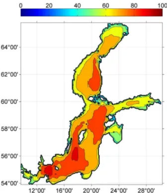
The basic features of the spatial pattern of numerically simulated average wave heights in the Baltic Sea over 38 years (1970–2007) qualitatively coincide with those discussed in Jönsson et al. (2002). The map of wave intensity in terms of the long-term average significant wave height (Fig. 9) is asymmetric with respect to the axis of the Bothnian Sea: its eastern part has clearly higher waves (>0.8 m on average) than its western area. The spatial pattern of the areas of large wave activity has several local maxima and is quite different for the southern and northern parts of the Baltic Proper.
The largest average wave heights occur south of Gotland and east of Öland (around 56°N, 18°E), and in the Arkona Basin, exceeding there 0.9 m over two areas of about 1° × 1° in size. The average wave height reaches 1.01 m at one location of relatively low depth in this
Fig. 9. Numerically simulated average significant wave height (colour bar, cm; isolines plotted after each 10 cm) in the Baltic Sea in 1970–2007.
basin. This is apparently caused by local wave focusing and is not representative of the entire southern Baltic Sea.
The wave activity in the NBP is the highest along the coasts of Estonia and Latvia. The wave heights are relatively low along the coasts of Lithuania, Kaliningrad district, and eastern Poland, although these areas have a relatively long fetch. The open part of the Bothnian Sea also has quite high waves. The overall wave intensity in the Gulf of Finland is clearly smaller. The average wave heights reach 0.7 m at its entrance and the central part but are about 0.6 m in the rest of this water body. These values match well a similar estimate for the vicinity of Tallinn Bay (0.56 m) based on one-point forcing of the WAM model with high-quality marine wind data (Soomere 2005). Riga Bay is even calmer with the average wave height slightly exceeding 0.6 m in the open sea.
Jönsson et al. (2002) demonstrated great seasonal variability of the monthly mean and maximum wave heights over the Baltic Sea. This is caused by a sub-stantial seasonal variation in the wind speed in this basin (Mietus 1998). The monthly mean wind speeds are usually the highest in autumn and early winter (October– January), while the mildest months are in late spring and early summer (Fig. 10). The variations in the monthly mean wind speed are about 60%: for example at Utö (1961–2001) the wind speed was about 5.3 m/s in May– July and >8.4 m/s in December, whereas the mean wind speed was 6.7 m/s.
As a first step towards quantification of seasonal variability in wave properties in the Baltic Sea, we compare the modelled, and observed or measured data. Seasonal variation in the monthly mean wave heights is clearly evident in wave fields recorded in the coastal areas of Estonia (Fig. 10). Wave intensity largely follows the seasonal pattern of the mean wind speed and is the highest in late autumn and early winter (December– January) and the smallest in late spring and summer (Soomere & Zaitseva 2007; Zaitseva-Pärnaste et al. 2009). This variation is generally adequately reproduced in numerical simulations of wave conditions (Jönsson et al. 2002; Räämet et al. 2009; Suursaar & Kullas 2009).
Fig. 10. (a) Seasonal variation in the monthly mean wind speed at Utö (1961–2001); (b) seasonal variation in the monthly mean wave height at Vilsandi (white bars: observations 1954– 2008, Zaitseva-Pärnaste 2009; grey bars: WAM model 1970– 2007).
of open sea waves (such as Vilsandi or Pakri) should be clearly more pronounced than the variations in wind speeds, because in many conditions (for example, fully developed wave systems) wave heights are proportional to the wind speed squared. This feature, however, is to some extent consistent with the fact that in many cases Baltic Sea wave systems are steeper than fully developed wave fields with the same wave height or period (Soomere 2008).
Seasonal variations in wave height at different off-shore sites in the Baltic Proper follow almost perfectly also the variations in the wind speed at Utö. The relative amplitude of the variation is almost the same from the southern part of the Baltic Sea up to the entrance to the Gulf of Finland.
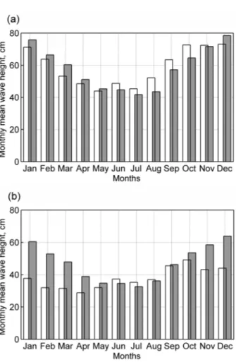
There are, however, some deviations of the seasonal variation in the measured and observed wave intensity from the pattern of the wind speed in coastal areas of Estonia and Sweden (Fig. 11). The data from the Gulf of
Fig. 11. Seasonal variation in the monthly mean wave height: (a) at Pakri (white bars: observations in 1954–85, Zaitseva-Pärnaste 2009; grey bars: WAM model 1970–2007); (b) at Narva-Jõesuu (white bars: observations 1954–2008, Zaitseva-Pärnaste 2009; grey bars: WAM model 1970–2007).
Finland reveal a secondary maximum in wave intensity in October, which is the overall maximum at Narva-Jõesuu. This feature is not evident at other sites (although relatively high wave activity in October can also be seen in the observed data from Vilsandi in Fig. 10) and thus can be attributed to the wave climate of the southern coast of the Gulf of Finland. The occurrence of relatively high waves compared to the monthly mean wind speed in early autumn (September–October) seems to be an overall feature of the wave climate in the NW coastal waters of Estonia. As it is much less clearly expressed starting from about 1980, it may partially be caused by the regular presence of the ice cover.
caused by local ageostrophic wind properties. The wind field of the central and western parts of the Gulf of Finland contains at times (especially in spring and early summer; Mietus 1998) quite strong eastern and western winds blowing along the axis of the gulf (Soomere & Keevallik 2003). This wind system is specific to the Gulf of Finland, not becoming evident in other parts of the Baltic Sea and being weaker in the eastern part of the gulf.
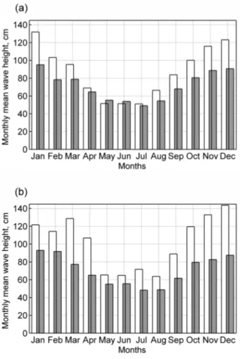
The rather large discrepancy between the measured and hindcast wave heights at Almagrundet (Table 1) is mostly caused by systematic overestimation of wave heights by the measurement devices during relatively windy months (Fig. 12). The measured and modelled wave heights almost coincide during the calmest months (May–July), especially in 1978–95. A minor difference is that the measured wave heights have a minimum value in May, but the calculated minimum is in July.
The wave intensity in March (and sometimes in April) was systematically higher than in February and even in
Fig. 12. Seasonal variation in the monthly mean wave height at Almagrundet: (a) 1978–95; (b) 1993–2003. White bars represent measured (Broman et al. 2006) and grey bars – modelled wave heights.
October in 1993–2003 at Almagrundet. This peculiarity is not present at other sites in the central and eastern parts of the Baltic Sea. One reason for this may be measurement noise, as discussed above. It may, however, be connected with the impact of easterly winds in years with a moderate ice cover. Such winds are generally relatively infrequent and weak in the NBP (Mietus 1998; Soomere & Keevallik 2001). Strong eastern winds may, as mentioned above, systematically occur during a few months in late winter and early spring in the NBP and especially in the Gulf of Finland (Soomere & Keevallik 2003). Note that the roughest wave conditions recorded in the northern Baltic Sea were measured at Almagrundet during an extreme eastern storm in 1984 (Broman et al. 2006).
STORMY AND CALM SEASONS
The above analysis reveals that during the first half of the year the model overestimates, and in the second half underestimates, the monthly mean wave heights at several wave observation sites (Figs 10 and 11). This peculiarity suggests that a phase shift (time lag, about one–two months) between the seasonal pattern of the wind speed and wave heights (and even more between the observed and modelled wave heights, Fig. 11a) occurs in the coastal areas of Estonia. In other words, the windiest season does not necessarily coincide with the season with the largest wave activity in the Baltic Sea. The physical reasons behind this feature are unclear. It may to some extent result from swells approaching from the southern Baltic Sea that are underestimated by the model. It is, however, unlikely that this effect would cause a time lag of about two months at Pakri. Further research is necessary in order to understand this feature and to capture it in models.
The time lag can roughly be estimated by means of separating the stormy and calm half-years. The five-month period from April to August is generally the calm time and five months from October to February are windy (Fig. 10a). The other two months serve as transient periods and may belong to either of the seasons.
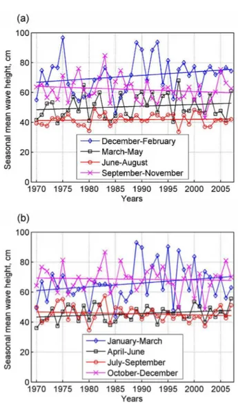
At Utö the windy and calm half-years are most clearly distinguished when September is allocated to the windy season and March to the calm season (Fig. 13). The average wind speed in the calm and windy seasons is 5.5 m/s and 8 m/s, respectively. Figure 13 also shows that the wind speed (in total about 2.5% annually) has increased at a more or less uniform rate of about 2% in March–November but much faster, about 3.5% annually during the second half of the windy half-year (December–February).
Fig. 13. Long-term trends in the wind speed in the windy and calm seasons at Utö for different dates of distinction between windy and calm seasons: (a) 1 September; (b) 1 October.
in Fig. 14 for the modelled wave heights. An attempt to separate the half-year of rough seas starting from September does not lead to a satisfactory result, as the wave intensity during the spring and autumn seasons differs insignificantly. On the other hand, wave conditions are, on average, clearly rougher during October–March (average about 0.7 m at Vilsandi) than in April–September when the average wave height is about 0.45 m.
Another, somewhat more exact estimate of the time lag between the overall patterns of seasonal variation in wind and wave conditions can be obtained by approximating the relevant variation with the periodic function f =αcos (2πt 12+β)+γ, where α expresses the amplitude of the annual variation in the property in question (wind speed or wave height), γ characterizes its annual average value, and β is the shift of its maximum from the beginning of the year. The para-meters of the best approximation can be determined, for example, in terms of the minimum root-mean- square deviation of the values of f( ,α β γ, , )ti from the relevant observed or modelled monthly mean values.
Fig. 14. Long-term trends in the modelled wave height in different seasons at Vilsandi for different dates of distinction between relatively rough and calm seasons: (a) 1 September; (b) 1 October.
Here ti, i=1,…, 12, are associated with the numbers
of the relevant months. The first approximations of the parameters α and γ are the total range of annual variation in the monthly means and the average annual value of the relevant property, respectively. The difference in the parameter β for different properties char-acterizes the time lag between their seasonal patterns. This difference is about half a month for the wind speed at Utö and the observed wave heights at Vilsandi, almost a month for the observed and modelled wave heights at Vilsandi, and about two months for the observed and modelled wave heights at Pakri.
gradually increased over this time. An increase in wave heights only becomes evident for early winter (December– February; Fig. 14), whereas during all other seasons almost no changes have taken place in wave intensity.
CONCLUSIONS AND DISCUSSION
The high-resolution long-term numerical simulations of the Baltic Sea wave properties with the use of adjusted geostrophic winds enabled us to estimate the basic characteristics of the northern Baltic Sea wave climatology over 38 years (1970–2007). The forcing with such wind fields normally does not allow exact reproduction of the details of wave fields but it is possible to establish reliably wave statistics. The simulations, however, qualitatively reproduced time series of wave properties without any systematic bias in areas open to predominant winds. The results match the long-term average wave height and basic properties of the seasonal pattern of wave intensity in the NBP and in the Gulf of Finland. The match is best for offshore sites and observation places open to the sea, and reasonable for sheltered areas.
The model and forcing used mostly overestimate the occurrence frequency of the most typical wave heights (0.25–0.75 m) for all analysed sites, both offshore and near the coast. The match is best for Pakri where wave observations have been performed in a relatively deep area adjacent to a high cliff.
The pattern of the average wave intensity over 38 years shows several areas with relatively high average wave heights. These areas in the eastern parts of the Bothnian Sea and the NBP match well the overall pattern of predominant westerly (mostly southwesterly) winds in the northern part of this water body. The presence of areas with relatively high waves south of Gotland and in the Arkona Basin suggests that southerly and easterly winds contribute substantially to the wave activity in the southern Baltic Sea. As a basic change in the wind climate of this area becomes evident as an increase in the strength and frequency of westerly winds (Pryor & Barthelmie 2003), the southern Baltic Sea may reveal very interesting patterns of change in the overall wave activity. Much of this change is likely to be concentrated in the winter (Pryor & Barthelmie 2003).
The seasonal pattern of wave activity, in general, follows a similar variation in the wind speed. The largest deviation of the measured or observed wave activity from the results of the numerical model is a secondary maximum of wave intensity in March at Almagrundet, probably caused by eastern storms in late winter in years with a small extension of the ice cover.
As such storms are inadequately represented in many numerical atmospheric models and as they apparently slow down when they reach the NBP (Soomere & Keevallik 2003), it is not unexpected that they are poorly represented in numerical simulations of wave fields based on geostrophic winds. Another feature not represented in numerical simulations is the relatively high wave activity in October at Pakri and Narva-Jõesuu. It is probably caused by strong autumn northwestern storms that, like many eastern storms in the Gulf of Finland, are locally generated (Soomere & Keevallik 2003; Savijärvi et al. 2005) and are poorly reproduced in atmospheric models and in geostrophic winds.
An interesting feature, the nature and extension of which need further research, is that calm and windy seasons for wind and wave conditions occur with a time lag of 0.5–2 months in the NBP. During the first half of the year the model overestimates and in the second half underestimates the monthly mean wave heights. Although this peculiarity may be the result of a too low resolution for the definition of the seasons, it still suggests that the wind speed is not the only factor controlling the wave height even in ice-free conditions. This conjecture is supported by the virtual absence of an increase in calculated wave heights in simulations under gradually increasing wind conditions (Suursaar et al. 2008; Räämet et al. 2009).
The reliability and causes of drastic variations in wave intensity at Almagrundet (Broman et al. 2006) and Vilsandi (Soomere & Zaitseva 2007) remain unclear. In the light of extensive evidence of substantial intensification of coastal processes on Saaremaa during the last decade (Orviku et al. 2003; Suursaar et al. 2008; Tõnisson et al. 2008) further research is necessary in order to clarify this problem.
an increase in the formal annual average wave height calculated on the basis of available observations (Type A statistics according to Kahma et al. 2003). This is consistent with the fact that the climatological mean wave height in months with frequent ice cover (January–March) is lower than the wave height in October–December. This conjecture, of course, does not mean that a decrease in the length of the ice period would lead to smaller overall wave loads to the coast. As the total wave impact covers all the days with waves, it is usually larger in years with less ice cover.
Acknowledgements. The authors are most grateful to the SMHI, especially to Dr Barry Broman, for providing help in retrieving the geostrophic wind data, to the EMHI for historical wave data and weather maps provided by Ivo Saaremäe, and to Inga Zaitseva-Pärnaste for providing digitized wave data from Vilsandi, Pakri, and Narva-Jõesuu. Heiko Herrmann and Loreta Kelpšaite are gratefully acknowledged for help with handling the CDO software. The study was supported by the Estonian Science Foundation (grant 7413), the Estonian Ministry of Education and Research (grant SF0140077s08), BONUS+ project Baltic Way, and the Marie Curie RTN project SEAMOCS (MRTN-CT-2005-019374). Useful comments by Dr Arno Behrens and an anonymous reviewer are thankfully appreciated.
REFERENCES
Ansper, I. & Fortelius, C. 2003. Verification of HIRLAM marine wind forecasts in the Baltic. Publicationes Instituti
Geographici Universitatis Tartuensis, 93, 195–204.
Bertotti, L. & Cavaleri, L. 2009. Wind and wave predictions in the Adriatic Sea. Journal of Marine Systems, 78, S227– S234.
Broman, B., Hammarklint, T., Rannat, K., Soomere, T. & Valdmann, A. 2006. Trends and extremes of wave fields in the north-eastern part of the Baltic Proper. Oceanologia, 48 (S), 165–184.
Bumke, K. & Hasse, L. 1989. An analysis scheme for determination of true surface winds at sea from ship synoptic wind and pressure observations.
Boundary-Layer Meteorology, 47, 295–308.
Cieślikiewicz, W. & Paplińska-Swerpel, B. 2008. A 44-year hindcast of wind wave fields over the Baltic Sea. Coastal
Engineering, 55, 894–905.
Elken, J., Raudsepp, U. & Soomere, T. 2002. On the current- and wave-induced sediment redistribution patterns in the Gulf of Riga. Terra Nostra, 4, 401–406.
Günther, H. & Rosenthal, W. 1995. Model Documentation of
HYPAS. Institut für Gewässerphysik. Abteilung GMS.
GKSS-Forschungszentrum Geesthacht GmbH, Geesthacht, Germany, 20 pp.
Häggmark, L., Ivarsson, K.-I., Gollvik, S. & Olofsson, P.-O. 2000. MESAN, an operational mesoscale analysis system.
Tellus, 52A, 2–20.
Jönsson, A. 2005. Model Studies of Surface Waves and
Sediment Resuspension in the Baltic Sea. PhD thesis.
Linköping Studies in Arts and Science, No. 332. Linköping University, 49 pp.
Jönsson, A., Broman, B. & Rahm, L. 2002. Variations in the Baltic Sea wave fields. Ocean Engineering, 30, 107–126. Jönsson, A., Danielsson, Å. & Rahm, L. 2005. Bottom type
distribution based on wave friction velocity in the Baltic Sea. Continental Shelf Research, 25, 419–435.
Kahma, K., Pettersson, H. & Tuomi, L. 2003. Scatter diagram wave statistics from the northern Baltic Sea. MERI – Report Series of the Finnish Institute of Marine
Research, 49, 15–32.
Keevallik, S. 2003. Possibilities of reconstruction of the wind regime over Tallinn Bay. Proceedings of the Estonian
Academy of Sciences, Engineering, 2003, 9, 209–219.
Keevallik, S., Männik, A. & Hinnov, J. 2010. Comparison of HIRLAM wind data with measurements at Estonian coastal meteorological stations. Estonian Journal of Earth
Sciences, 59, 90–99.
Kelpšaite, L., Herrmann, H. & Soomere, T. 2008. Wave regime differences along the eastern coast of the Baltic Proper. Proceedings of the Estonian Academy of Sciences, 57, 225–231.
Kelpšaite, L., Parnell, K. E. & Soomere, T. 2009. Energy pollution: the relative influence of wind-wave and vessel-wake energy in Tallinn Bay, the Baltic Sea.
Journal of Coastal Research, Special Issue 56, vol. 1,
812–816.
Komen, G. J., Cavaleri, L., Donelan, M., Hasselmann, K., Hasselmann, S. & Janssen, P. A. E. M. 1994. Dynamics
and Modelling of Ocean Waves. Cambridge University
Press, 532 pp.
Kriezi, E. E. & Broman, B. 2008. Past and future wave climate in the Baltic Sea produced by the SWAN model with forcing from the regional climate model RCA of the Rossby Centre. In IEEE/OES US/EU-BalticInternational
Symposium, May 27–29, 2008, Tallinn, Estonia, pp. 360–
366. IEEE.
Kull, A. 2005. Relationship between interannual variation of wind direction and wind speed. Publicationes Instituti
Geographici Universitatis Tartuensis, 97, 62–73.
Lopatukhin, L. I., Bukhanovsky, A. V., Ivanov, S. V. & Tshernyshova E. S. (eds). 2006. Spravochnye dannye po rezhimu vetra i volneniya Baltijskogo, Severnogo,
Azovskogo i Sredizemnego morej [Handbook of wind
and wave regimes in the Baltic Sea, North Sea, Black
Sea, Azov Sea and the Mediterranean]. Russian Shipping
Registry, St. Petersburg, 450 pp. [in Russian].
Mietus, M. (co-ordinator). 1998. The Climate of the Baltic Sea
Basin. Marine meteorology and related oceanographic
activities, Report No. 41, World Meteorological Organi-sation, Geneva, 64 pp.
Orviku, K., Jaagus, J., Kont, A., Ratas, U. & Rivis, R. 2003. Increasing activity of coastal processes associated with climate change in Estonia. Journal of Coastal Research, 19, 364–375.
Pryor, S. C. & Barthelmie, R. J. 2003. Long-term trends in near-surface flow over the Baltic. International Journal
of Climatology, 23, 271–289.
Räämet, A., Suursaar, Ü., Kullas, T. & Soomere, T. 2009. Reconsidering uncertainties of wave conditions in the coastal areas of the northern Baltic Sea. Journal of
Savijärvi, H., Niemela, S. & Tisler, P. 2005. Coastal winds and low-level jets: simulations for sea gulfs. Quarterly
Journal of the Royal Meteorological Society, B, 131(606),
625–637.
Seifert, T., Tauber, F. & Kayser, B. 2001. A high resolution
spherical grid topography of the Baltic Sea, 2nd edition.
Baltic Sea Science Congress, Stockholm 25–29 November 2001, Poster 147.
Signell, R. P., Carniel, S., Cavaleri, L., Chiggiato, J., Doyle, J. D., Pullen, J. & Sclavo, M., 2005. Assessment of wind quality for oceanographic modelling in semi-enclosed basins. Journal of Marine Systems, 53(1–4), 217–233.
Sooäär, J. & Jaagus, J. 2007. Long-term changes in the sea ice regime in the Baltic Sea near the Estonian coast. Proceedings of the Estonian Academy of Sciences,
Engineering, 13, 189–200.
Soomere, T. 2001. Wave regimes and anomalies off north-western Saaremaa Island. Proceedings of the Estonian
Academy of Sciences, Engineering, 7, 157–173.
Soomere, T. 2003. Anisotropy of wind and wave regimes in the Baltic Proper. Journal of Sea Research, 49, 305–316. Soomere, T. 2005. Wind wave statistics in Tallinn Bay. Boreal
Environmental Research, 10, 103–118.
Soomere, T. 2008. Extremes and decadal variations of the northern Baltic Sea wave conditions. In Extreme Ocean
Waves (Pelinovsky, E. & Kharif, Ch., eds), pp. 139–157.
Springer, New York.
Soomere, T. & Keevallik, S. 2001. Anisotropy of moderate and strong winds in the Baltic Proper. Proceedings of the
Estonian Academy of Sciences, Engineering, 7, 35–49.
Soomere, T. & Keevallik, S. 2003. Directional and extreme wind properties in the Gulf of Finland. Proceedings of the
Estonian Academy of Sciences, Engineering, 9, 73–90.
Soomere, T. & Zaitseva, I. 2007. Estimates of wave climate in the northern Baltic Proper derived from visual wave
observations at Vilsandi. Proceedings of the Estonian
Academy of Sciences, Engineering, 13, 48–64.
Soomere, T., Behrens, A., Tuomi, L. & Nielsen, J. W. 2008. Wave conditions in the Baltic Proper and in the Gulf of Finland during windstorm Gudrun. Natural Hazards and
Earth System Sciences, 8, 37–46.
Sterl, A. & Caires, S. 2005. Climatology, variability and extrema of ocean waves – the web-based KNMI/ERA-40 wave atlas. International Journal of Climatology, 25, 963–977.
Suursaar, Ü. & Kullas, T. 2009. Decadal variations in wave heights off Cape Kelba, Saaremaa Island, and their relationships with changes in wind climate. Oceanologia, 51, 39–61.
Suursaar, Ü., Jaagus, J., Kont, A., Rivis, R. & Tõnisson, H. 2008. Field observations on hydrodynamic and coastal geomorphic processes off Harilaid Peninsula (Baltic Sea) in winter and spring 2006–2007. Estuarine Coastal and
Shelf Science, 80, 31–41.
Tõnisson, H., Orviku, K., Jaagus, J., Suursaar, Ü., Kont, A. & Rivis, R. 2008. Coastal damages on Saaremaa Island, Estonia, caused by the extreme storm and flooding on January 9, 2005. Journal of Coastal Research, 24, 602– 614.
Tuomi, L., Pettersson, H. & Kahma, K. 1999. Preliminary results from the WAM wave model forced by the mesoscale EUR-HIRLAM atmospheric model. MERI –
Report series of the Finnish Institute of Marine Research,
40, 19–23.
Zaitseva-Pärnaste, I. 2009. Long-term Variations of Wave
Fields in the Estonian Coastal Waters. MSc Thesis.
Tallinn, 2009, 67 pp.
Zaitseva-Pärnaste, I., Suursaar, Ü., Kullas, T., Lapimaa, S. & Soomere, T. 2009. Seasonal and long-term variations of wave conditions in the northern Baltic Sea. Journal of
Coastal Research, Special Issue 56, vol. 1, 277–281.