J. Braz. Chem. Soc. vol.24 número12

Article

Printed in Brazil - ©2013 Sociedade Brasileira de Química 0103 - 5053 $6.00+0.00

A

*e-mail: jaagredab@unal.edu.co

Bursting in the Belousov-Zhabotinsky Reaction Added with

Phenol in a Batch Reactor

Ariel Cadena,

Daniel Barragán

and Jesús Ágreda*

a

_{Departamento de Química, Facultad de Ciencias, Universidad Nacional de Colombia,}

Cra 30 No. 45-03, Bogotá, Colombia

b

_{Escuela de Química, Facultad de Ciencias, Universidad Nacional de Colombia,}

Calle 59A No. 63-20, Oficina 16-413, Medellín, Colombia

A reação de Belousov-Jabotinsky clássica foi modificada pela adição de fenol como um segundo substrato orgânico que compete cineticamente com o ácido malônico na redução de Ce4+ _{para Ce}3+ _e

na remoção de bromo molecular da reação. A reação oscilante de dois substratos exibiu oscilações abruptas e período oscilatório de longa duração. A análise de dados experimentais mostra um aumento do fenômeno abrupto, com pico maior e estado quiescente mais longo, como função do aumento da concentração de fenol inicial. Hipotetizou-se que o fenômeno de oscilação abrupta pode ser explicado pela introdução de um ciclo redox entre as espécies fenólicas reduzidas (hidroxifenois) e as oxidadas onas (quinonas). A hipótese foi testada experimentalmente e numericamente e dos resultados concluiu-se que o fenômeno oscilatório abrupto exibido pela reação oscilante de dois substratos é impulsionado principalmente por um ciclo redox p-di-hidroxi-benzeno/p-benzoquinona.

The classic Belousov-Zhabotinsky reaction was modified by adding phenol as a second organic substrate that kinetically competes with the malonic acid in the reduction of Ce4+ _{to Ce}3+ _{and in the}

removal of molecular bromine of the reaction mixture. The oscillating reaction of two substrates exhibited burst firing and an oscillatory period of long duration. Analysis of experimental data shows an increasing of the bursting phenomenon, with a greater spiking in the burst firing and with a longer quiescent state, as a function of the initial phenol concentration increase. It was hypothesized that the bursting phenomenon can be explained introducing a redox cycle between the reduced phenolic species (hydroxyphenols) and the oxidized ones (quinones). The hypothesis was experimentally and numerically tested and from the results it is possible to conclude that the bursting phenomenon exhibited by the oscillating reaction of two substrates is mainly driven by a p-di-hydroxy-benzene/p-benzoquinone redox cycle.

Keywords: reaction kinetics, mechanisms, phenolic compounds, BZ reaction, bursting phenomenon

Introduction

The Belousov-Zhabotinsky (BZ) and uncatalyzed

bromate oscillator (UBO) reactions have been studied in a

wide of experimental conditions in both batch and continuous

stirred tank (CSTR) reactors.

_{Complex dynamic behaviors}

in oscillating reactions have been found in non-stirred batch

reactors and in CSTR and electrochemical setups.

_These

amazing reactions have become relevant in science, and

particularly in biochemistry, due to their similarity with

the dynamic activity of many cellular control processes.

On the other hand, travelling waves, Turing patterns, burst

firing, sequential oscillations and chaotic phenomena are

some of the more common spatio-temporal dynamics

studied in oscillating reactions.

_{Looking for a better}

understanding of the reaction mechanism and dynamics

of oscillating reactions, researchers have employed several

substrates, individually or mixed, in the study of BZ reaction.

The induction period, frequency, amplitude, shape and

periodicity of oscillations change by the presence of a new

organic or inorganic substance in the reaction mixture of

BZ reaction.

bromated in sulfuric acidic) were studied in a batch reactor

in the presence of phenol as a second organic substrate

that kinetically competes with the malonic acid in the

reduction of Ce

_{to Ce}

_{and in the removal of molecular}

bromine. With the two substrates (malonic acid-phenol),

BZ reaction shows an astonishing variation of its dynamics

as a function of the initial concentration of phenol,

exhibiting enhanced periods of oscillations and bursting

phenomenon. At first glance, the malonic acid-phenol BZ

oscillator was thought as a system of coupled oscillators

because the bromate-phenol-sulfuric acidic is a well-known

oscillating chemical reaction (UBO). In order to test this

idea of coupled oscillators, a set of numerical simulations

by using an extended reaction mechanism based on the

Marburg-Budapest-Missoula (MBM)

_{and Gyorgyi, Varga,}

Körös, Field and Ruoff (GVKFR)

_{reaction schemes was}

carried out. The MBM mechanism for the cerium-catalyzed

BZ reaction is a complete reaction scheme that includes both

negative feedback loops and radical-radical recombination

reactions of organic species.

_{Whereas the GVKFR model}

is a mechanism to explain the oscillations observed in the

p

-hydroxyphenol-bromate-acidic media reaction,

_the

closer and complete mechanism available in the literature

to UBO that uses phenol as organic substrate. As a result

of these numerical simulations, some interesting behaviors

were obtained, but there was nothing to indicate the

possibility of burst firing.

In order to address the experimental evidence of that

burst firing obtained in this work for the malonic acid-phenol

BZ reaction, a second hypothesis is that the subproducts of

phenol oxidation (hydroxyphenols-quinones) are involved

in a novel redox cycle coupled to the main catalytic cycle of

cerium ions. A series of experiments using 1,4-benzoquinone,

2-hydroxyphenol and 4-hydroxyphenol instead of phenol

as a second organic substrate were carried out to test this

hypothesis. The experimental results obtained by adding

benzoquinone and hydroxyphenols to the BZ reaction

suggest that the hypothesized hydroxyphenol-quinone

redox cycle can be accepted as plausible. This hypothesis

was materialized as a set of reaction steps, and they were

incorporated into an extended MBM-GVKFR mechanism.

The numerical simulation results of this new model

(MBM-GVKFR-hydroxyphenols-quinones redox cycle)

support the idea of the hydroxyphenols-quinones redox

cycle.

Experimental

S u l f u r i c a c i d ( M e r c k 9 5 - 9 8 % ex t r a p u r e ) ,

KBrO

(Carlo Erba Milano ACS Titolo min 99.8%),

Ce(SO

)

4H

O (Merck zur Analyse > 98%), malonic

acid (Merck zur Synthese), phenol (JT Baker Chemicals

B. V. “Baker Grade”), 2-hydroxyphenol (Fisher Scientific

Company), 4-hydroxyphenol (Merck zur Synthese) and

p

-benzoquinone (Hopkin and Williams, LTD.) were used

as received. All solutions were prepared in deionized water.

The initial concentration of phenol used in the experiments

were: a. 0.00, b. 0.05347, c. 0.1337, d. 0.2673, e. 0.5347,

f. 1.069, g. 1.337, h. 1.604, i. 1.871, j. 2.272, k. 2.673,

l. 3.074, m. 3.476, n. 3.877, o. 4.278, p. 4.679, q. 5.347, and

r. 10.69 mmol L

_{. The initial concentrations of classic BZ}

reagents were: 28.90 mmol L

_KBrO

3

, 26.06 mmol L

malonic acid, 0.5606 mmol L

_Ce(SO

4

)

and 1.00 mol L

H

SO

. A thermostated (25.0 ± 0.1

C) 100 mL double jacket

cylindrical cell, with magnetic stirring at 500 rpm, was

used to obtain the potentiometric measurements, using a

platinum electrode Mettler-Toledo Pt4805-60-88TE-S7/120

combination ORP/Redox with Ag/AgCl reference (movable

PTFE reference junction). All the experiments were made

at least by duplicate.

Results and Discussion

The malonic acid-phenol BZ reaction exhibits a striking

alteration of its temporal oscillatory dynamics as a function

of the initial concentration of phenol. An enlargement of the

oscillatory regime and the onset of bursting phenomenon

are the more important observed effects by the addition of

phenol to BZ reaction. The length of the induction time,

the amplitude of sustained oscillations and the increasing

of the total oscillatory reaction time are closely correlated

with the initial concentration of phenol, and the burst firing

appears when the malonic acid-phenol concentration ratio

ranges between 25 and 6. Figure 1 shows the temporal

redox potentiometric measurements of BZ reaction

in the presence of an initial concentration of phenol

(curves a to r). The BZ reaction (Figure 1 curve a) has an

oscillatory reaction time of around 2 h, while at the same

initial concentrations but in the presence of 3.074 mmol L

phenol (Figure 1 curve l), the oscillatory reaction time

extends to almost 30 h.

Figure 1 also shows other highlighting features of

this BZ oscillating reaction of two substrates. When the

initial concentration of phenol is lower than 2.0 mmol L

(Figure 1 curves from a to i), the reaction mixture exhibits

sustained oscillatory phase, and the period and the

amplitude of the oscillations remain constant before a

sudden ending. If the initial concentration of phenol, ranges

between 2.0 and 10 mmol L

_{(Figure 1 curves j to q), the}

of BZ reaction was the bursting phenomenon. If the

initial concentration of phenol ranges between 1.069 and

3.476 mmol L

_{(Figure 1 curves f to m), the reaction}

mixture exhibits a complex temporal transition from burst

firing and sustained oscillations (ended suddenly), to still

burst firing but damped oscillations. This means that the

malonic acid-phenol BZ reaction in a batch reactor evolves

in time through different attractors: period-n bursting

attractor, limit cycle and stable focus.

In order to explain the experimental results showed in

Figure 1, a new redox cycle is propose: the Ce

_oxidation

of phenol to

p

-quinones

_{followed by the reduction of}

p

-quinones to phenolic compounds mediated by transient

reactive organic free radicals in solution,

_{like carboxyl}

(COOH

_{) or tartronyl (TA}

_).

_{If this aromatic redox}

cycle is plausible, then the Ce

_/Ce

_{catalytic cycle of BZ}

reaction is involved in a kinetic competition, the reduction

of BrO

by Ce

or phenol. In a typical antioxidation action,

common in phenols, the oxidation of Ce

_{is diminished, and}

because of this, the consumption of malonic acid is slower,

whereas the phenol consumption is higher. These facts

together increase the oscillation time of the BZ reaction

of two substrates. Now, at low concentration of phenolic

compounds, the Ce

_{concentration rises, and the Ce}

_/Ce

catalytic cycle drives the BZ reaction while quinone type

compounds are reduced to phenolic compounds by some

reactive free radicals, like the carboxyl (COOH

_{) or the}

tartronyl (TA

_{) radicals. When the concentration of phenolic}

compounds increases, the aromatic cycle (phenol-quinone)

restarts and drives the oscillating reaction. In this way,

it is proposed that the two catalytic cycles alternate to

drive the reaction until the oscillatory period ends. It is

important to take into account that the polymerization of

the quinones takes place at the reaction mixture conditions,

as it is well-known from the UBO chemical oscillator.

The polymers of quinone are almost insoluble and their

reduction by free radicals is not a viable process and we

suppose that they are involved in the burst firing by way of

a non-synchronized action between catalytic processes. It is

also important to remark that at high enough concentration

of phenol, the Ce

_{oxidation of phenolic compounds is a}

kinetically preferred process, instead of the Ce

_oxidation

of aliphatic species of the BZ reaction.

All the above ideas have the aim to help to understand,

from a mechanistic point of view, the complex behavior

exhibited by the malonic acid-phenol BZ oscillating

reaction, and those ideas are summarized in the next

way: at the beginning of reaction, the oxidation of phenol

by Ce

_{is the kinetically favored process with a slow}

consumption of bromate and malonic acid; in this way,

whereas the concentration of phenolic compounds is over

a critical value, the aromatic catalytic cycle drives BZ

oscillations; and when the phenol concentration is high

enough, insoluble polymers of quinone are produced and

an irregular oscillatory dynamic appears, the bursting

phenomenon. At long times, the phenolic compounds are

decreased in the reaction mixture, and a sequential train

of sustained oscillations, driven by the consumption of

malonic acid by the Ce

_/Ce

_{catalytic cycle, leads the}

oscillations to its end.

In order to get some experimental clues about the

participation of phenol in the malonic acid BZ reaction,

the classic experiment was tested in the presence of

some key aromatic compounds, 2-hydroxyphenol,

4-hydroxyphenol and

p

-benzoquinone. The results are in

Figure 2, in which curves c and e show that the BZ reaction

of two substrates (malonic acid with

p

-benzoquinone and

malonic acid with

4

-hydroxyphenol, respectively) exhibits

a dynamic behavior of a similar type that the malonic acid

with phenol, curve b. On the contrary, the

2

-hydroxyphenol,

curve d, does not modify, to an appreciable extent, the

malonic acid BZ reaction, curve a. The main result in

Figure 2 is the evidence suggesting that the proposal, about

the oxidation-reduction cycle, among phenol and quinone

compounds, is capable to explain the experimental results.

Also, it says that the main compound in the phenol-quinone

process is a

para

compound and not an

orto

compound, as

could be inferred from UBO oscillators.

Numerical simulations

Numerical simulations were used as a tool to treat

the fully nonlinear dynamics of the complex chemical

BZ reaction

and to test the validity of the previously

presented hypothesis. The following set of reactions 1 to 9

was added to the complete set of reactions of MBM plus

the GVKFR mechanisms (the complete set of reaction

rates, kinetic constants and the fortran source code used

for these simulations are presented in the Supplementary

Information (SI) section).

Phenol oxidation reactions:

(1)

(2)

(3)

(4)

Quinone reduction reactions:

(5)

(6)

(7)

(8)

Quinone consumption:

(9)

In these reactions,

TA is for tartronic acid and MOA is

for meso-oxalic acid.

_{The rate constants were estimated}

based on similar reactions of the MBM and GVKFR

mechanisms. Reactions 1 to 4 describe a sequential electron

transfer for the Ce

_{and the resulting oxidation of phenol}

to the corresponding quinone. Reactions 5 to 8 indicate

a plausible sequential reduction of quinone, by reactive

organic free radicals, to phenolic like compounds. The

selection of free radical species involved in reactions 5 to 8

was based on redox potentials. The carboxyl radical

(COOH

_{) has a standard redox potential of}

−

1.82 V

vs

.

NHE.

_{On the other hand, the tartronyl radical (TA}

_{) was}

chosen as a representative free radical that has been found

in the BZ reaction (like the malonyl and bromomalonyl

free radicals).

_{Finally, the reaction 9 describes the}

irreversible degradation or polymerization of quinones.

Figure 3 shows the results obtained for simulations.

The numerical simulations have some of the experimental

observed characteristics of the malonic acid-phenol BZ

oscillating reaction, like an induction time enlargement and

an increasing oscillatory reaction time as the initial phenol

concentration increases. Also, the burst firing appears, and

it is the most interesting result (inset in Figure 3). This

qualitative agreement, between the experiments and the

numerical simulations, is in favor of the hypothesized

phenol-quinone redox cycle. However, it is necessary to

confirm these ideas, in future works, by determining the

experimental rate constant values, and by including, or

deleting, some reactions. Also, a chromatographic and

electron paramagnetic resonance (EPR) spectroscopy

studies would be particularly useful to find the specific

intermediaries.

Conclusions

The results presented in this work show the dynamic

behavior of the malonic acid-phenol BZ reaction. It is

interesting the appearance of bursting phenomenon in a

Figure 2. Redox potentiometric signal against time for the BZ oscillating reaction of two substrates. a: malonic acid alone, b: malonic acid with phenol, c: malonic acid with 1,4-benzoquinone, d: malonic acid with 2-hydroxyphenol, and e: malonic acid with 4-hydroxyphenol. The phenolic species were added in concentration of 1.3 mmol L-1_{. The other}

concentrations were the same as in Figure 1.

closed system. The burst firing origin was explained as a

complex process that involves a kinetic competition between

an aromatic redox cycle of phenolic compounds and the

Ce

_/Ce

_{catalytic cycle of the BZ classic oscillator. In this}

way, the presence of phenol in the malonic acid BZ reaction

plays a role as an antioxidant agent preventing the oxidation

of the malonic acid, and its derivatives, by Ce

_ions.

Supplementary Information

Supplementary data are available free of charge at

http://jbcs.sbq.org.br as PDF file.

Acknowledgment

This project has been supported by the DIB of the

Universidad Nacional de Colombia under the code 803638.

Reference

1. Sagués, F.; Epstein, I. R.; Dalton Trans. 2003, 7, 1201. 2. Básángi, T.; Leda, M. Jr.; Toiya, M.; Zhabotinsky, A. M.;

Epstein, I. R.; J. Phys. Chem. A 2009, 113, 5644.

3. Gentili, P. L.; Horvath, V.; Vanag, V. K.; Epstein, I. R.; Int. J. Unconv. Comput. 2012, 8, 177.

4. Adamciková, L.; Misicák, D.; Sevcik, P.; React. Kinet. Catal. Lett. 2005, 85, 215.

5. Szabo, E.; Adamciková, L.; Sevcik, P.; J. Phys. Chem. A 2011, 115, 6518.

6. Ruoff, P.; J. Phys. Chem. 1992, 96, 9104.

7. Grancicova, O.; Olexova, A.; Z. Phys. Chem. 2009, 223, 1451. 8. Rachwalska, M.; Kawczynski, A. L.; J. Phys. Chem. A 2001,

105, 7885.

9. Badola, P.; Rajani, P.; Ravi-Kumar, V; Kulkarni, B. D.; J. Phys. Chem. 1991, 9, 2939.

10. Bronnikova, T. V.; Schaffer, W. M.; Olsen, L. F.; J. Phys. Chem. B 2001, 105, 310.

11. Kiss, I. Z.; Lv, Q.; Organ, L.; Hudson, J. L.; Phys. Chem. Chem. Phys. 2006, 8, 2707.

12. Simo, H.; Woafo, P.; Mech. Res. Comm. 2011, 38, 537. 13. Izhikevich, E. M.; Int. J. Bifurcation Chaos 2000, 10, 1171. 14. Lengyel, I.; Epstein, I. R.; Acc. Chem. Res. 1993, 26, 235. 15. Epstein, I. R.; Showalter, K.; J. Phys. Chem. 1996, 100, 13132. 16. Epstein, I. R.; Pojman, J. A.; An Introduction to Nonlinear

Chemical Dynamics; Oxford University Press: New York, USA, 1998.

17. Rastogi, R. P.; Introduction to Non-Equilibrium Physical Chemistry; Elsevier: Amsterdam, The Netherlands, 2008.

18. Pojman, J. A.; Tran-Cong-Miyata, Q.; Nonlinear Dynamics with Polymers; Wiley-VCH Velarg: Weinheim, Germany, 2010. 19. Heilweil, E. J.; Henchman, M. J.; Epstein, I. R.; J. Am. Chem.

Soc. 1979, 101, 3698.

20. Treindl, L.; Ruoff, P.; Kvernberg, P. O.; J. Phys. Chem. A 1997, 101, 4606.

21. Rastogi, R. P.; Chand, P.; Pandey, M. K.; Das, M.; J. Phys. Chem. A 2005, 109, 4562.

22. Shah, S.; Wang, J.; J. Phys. Chem. C 2007, 111, 10639. 23. Zeyer, K.-P.; Schneider, F. W.; J. Phys. Chem. A 1998, 102,

9702.

24. Chen, Y.; Wang, J.; J. Phys. Chem. A 2005, 109, 3950. 25. Amemiya, T.; Wang, J.; J. Phys. Chem. A 2010, 114, 13347. 26. Schwarz, H. A.; Dodson, R. W.; J. Phys. Chem. 1989, 93, 409. 27. Li, N.; Wang, J.; J. Phys. Chem. A 2008, 112, 6281.

28. Biosa, G.; Ristori, S.; Spalla, O.; Rustici, M.; Hauser, M. J. B.; J. Phys. Chem. A. 2011, 115, 3227.

29. Asakura, K.; Konishi, R.; Nakatani, T.; Nakano, T.; Kamata, M.; J. Phys. Chem. B 2011, 115, 3959.

30. Gyorgyi, L.; Turányi. T.; Field, R. J.; J. Phys. Chem. 1990, 94, 7162.

31. Gyorgyi, L.; Turányi, T.; Field, R. J.; J. Phys. Chem. 1993, 97, 1931.

32. Hegedeus, L.; Wittman, M.; Noszticzius, Z.; Yan, S.; Sirimungkala, A.; Försterling, H. D.; Field, R. J.; Faraday Discuss. 2002, 120, 21.

33. Györgyi, L.; Varga, M.; Körös, E.; Field, R. J.; Ruoff, P.; J. Phys. Chem. 1989, 93, 2836.

34. Spence, W. R.; Duke, F. R.; Anal. Chem. 1954, 26, 919. 35. Dixon, W. T.; Murphy, D.; J. Chem. Soc., Perkin Trans. 1975,

2, 850.

36. Domagała, S.; Steglińska, V.; Dziegieć, J.; Monatsh. Chem. Chem. Mon. 1998, 129, 761.

37. Simon, A.; Ballai, C.; Lente, G.; Fábián, I.; New. J. Chem. 2011, 35, 235.

38. Wardman, P.; Reduction Potentials of One-Electron Couples Involving Free Radicals in Aqueous Solution; American Chemical Society and the American Institute of Physics for the National Institute of Standards and Technology: USA, 1989, p. 1637.

39. Blagojevic, S. M.; Anic, S. R.; Cupic, Z. D.; Russ. J. Phys. Chem. A 2011, 85, 2274.

40. Singh, M. P.; Singh, H. S.; Verma, M.; J. Phys. Chem. 1980, 84, 256.

Submitted: July 27, 2013

Supplementary Information

S

I

*e-mail: jaagredab@unal.edu.co

Bursting in the Belousov-Zhabotinsky Reaction Added with

Phenol in a Batch Reactor

Ariel Cadena,

Daniel Barragán

and Jesús Ágreda*

a

_{Departamento de Química, Facultad de Ciencias, Universidad Nacional de Colombia,}

Cra 30 No. 45-03, Bogotá, Colombia

b

_{Escuela de Química, Facultad de Ciencias, Universidad Nacional de Colombia,}

Calle 59A No. 63-20, Oficina 16-413, Medellín, Colombia

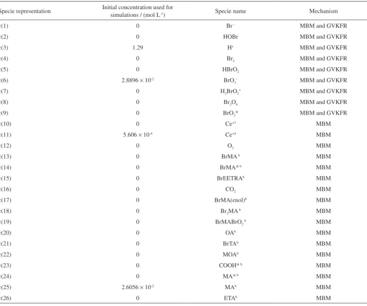
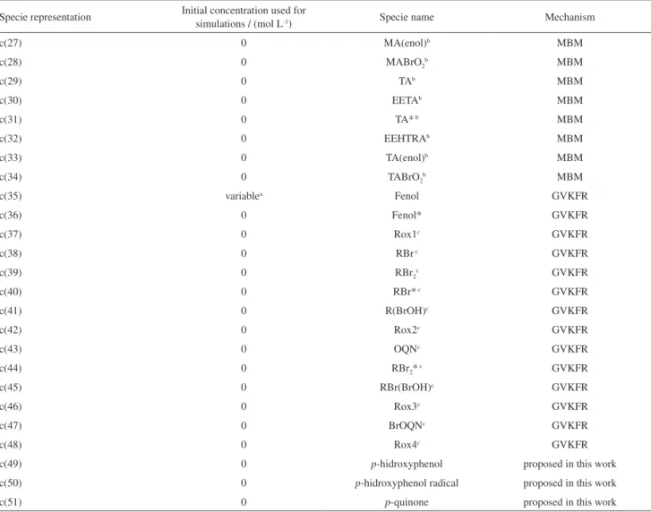
Table S1. Species nomenclature and initial concentrations used for the simulation of the BZ reaction added with phenol

Specie representation Initial concentration used for

simulations / (mol L-1₎ Specie name Mechanism

c(1) 0 Br– _{MBM and GVKFR}

c(2) 0 HOBr MBM and GVKFR

c(3) 1.29 H+ _{MBM and GVKFR}

c(4) 0 Br2 MBM and GVKFR

c(5) 0 HBrO₂ MBM and GVKFR

c(6) 2.8896 × 10-2 BrO3– MBM and GVKFR

c(7) 0 H2BrO2+ MBM and GVKFR

c(8) 0 Br₂O₄ MBM and GVKFR

c(9) 0 BrO₂* MBM and GVKFR

c(10) 0 Ce+3 _MBM

c(11) 5.606 × 10-4 Ce+4 MBM

c(12) 0 O2 MBM

c(13) 0 BrMA b _MBM

c(14) 0 BrMA* b _MBM

c(15) 0 BrEETRAb _MBM

c(16) 0 CO₂ MBM

c(17) 0 BrMA(enol)b _MBM

c(18) 0 Br₂MA b _MBM

c(19) 0 BrMABrO₂ b _MBM

c(20) 0 OAb _MBM

c(21) 0 BrTAb _MBM

c(22) 0 MOAb _MBM

c(23) 0 COOH* b _MBM

c(24) 0 MA* b _MBM

c(25) 2.6056 × 10-2 _MAb _MBM

Specie representation Initial concentration used for

simulations / (mol L-1₎ Specie name Mechanism

c(27) 0 MA(enol)b _MBM

c(28) 0 MABrO₂b _MBM

c(29) 0 TAb _MBM

c(30) 0 EETAb _MBM

c(31) 0 TA* b _MBM

c(32) 0 EEHTRAb _MBM

c(33) 0 TA(enol)b _MBM

c(34) 0 TABrO2b MBM

c(35) variablea _{Fenol GVKFR}

c(36) 0 Fenol* GVKFR

c(37) 0 Rox1c _GVKFR

c(38) 0 RBr c _GVKFR

c(39) 0 RBr2c GVKFR

c(40) 0 RBr* c _GVKFR

c(41) 0 R(BrOH)c _GVKFR

c(42) 0 Rox2c _GVKFR

c(43) 0 OQNc _GVKFR

c(44) 0 RBr₂* c _GVKFR

c(45) 0 RBr(BrOH)c _GVKFR

c(46) 0 Rox3c _GVKFR

c(47) 0 BrOQNc _GVKFR

c(48) 0 Rox4c _GVKFR

c(49) 0 p-hidroxyphenol proposed in this work

c(50) 0 p-hidroxyphenol radical proposed in this work

c(51) 0 p-quinone proposed in this work

a_{Everyone of the 18 experimental concentrations of phenol was used here.} b_{The nomenclature use in references 32 of the paper was used.} c_{The nomenclature}

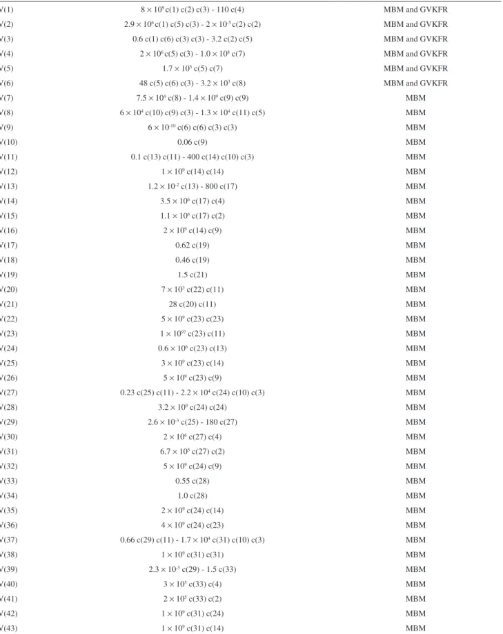
Table S2. The complete set of reaction rates used for the simulation of the bursting phenomena in the BZ reaction added with phenol. The numerical values are the respective kinetic constants. The negative sign precedes the reverse reaction when the reverse kinetic constant is different to zero

Reaction Reaction rate Mechanism

V(1) 8 × 109 c(1) c(2) c(3) - 110 c(4) MBM and GVKFR

V(2) 2.9 × 106 _{c(1) c(5) c(3) - 2}

× 10-5 _{c(2) c(2) MBM and GVKFR}

V(3) 0.6 c(1) c(6) c(3) c(3) - 3.2 c(2) c(5) MBM and GVKFR

V(4) 2 × 106 _{c(5) c(3) - 1.0}

× 108 _{c(7) MBM and GVKFR}

V(5) 1.7 × 105 _{c(5) c(7) MBM and GVKFR}

V(6) 48 c(5) c(6) c(3) - 3.2 × 103 c(8) MBM and GVKFR

V(7) 7.5 × 104 _{c(8) - 1.4}

× 109 _{c(9) c(9) MBM}

V(8) 6 × 104 _{c(10) c(9) c(3) - 1.3 × 10}4 _{c(11) c(5) MBM}

V(9) 6 × 10-10 c(6) c(6) c(3) c(3) MBM

V(10) 0.06 c(9) MBM

V(11) 0.1 c(13) c(11) - 400 c(14) c(10) c(3) MBM

V(12) 1 × 109 _{c(14) c(14) MBM}

V(13) 1.2 × 10-2 _{c(13) - 800 c(17) MBM}

V(14) 3.5 × 106 c(17) c(4) MBM

V(15) 1.1 × 106 _{c(17) c(2) MBM}

V(16) 2 × 109 c(14) c(9) MBM

V(17) 0.62 c(19) MBM

V(18) 0.46 c(19) MBM

V(19) 1.5 c(21) MBM

V(20) 7 × 103 _{c(22) c(11) MBM}

V(21) 28 c(20) c(11) MBM

V(22) 5 × 109 c(23) c(23) MBM

V(23) 1 × 1097 _{c(23) c(11) MBM}

V(24) 0.6 × 106 c(23) c(13) MBM

V(25) 3 × 109 _{c(23) c(14) MBM}

V(26) 5 × 109 _{c(23) c(9) MBM}

V(27) 0.23 c(25) c(11) - 2.2 × 104 c(24) c(10) c(3) MBM

V(28) 3.2 × 109 _{c(24) c(24) MBM}

V(29) 2.6 × 10-3 c(25) - 180 c(27) MBM

V(30) 2 × 106 c(27) c(4) MBM

V(31) 6.7 × 105 _{c(27) c(2) MBM}

V(32) 5 × 109 c(24) c(9) MBM

V(33) 0.55 c(28) MBM

V(34) 1.0 c(28) MBM

V(35) 2 × 109 c(24) c(14) MBM

V(36) 4 × 109 _{c(24) c(23) MBM}

V(37) 0.66 c(29) c(11) - 1.7 × 104 c(31) c(10) c(3) MBM

V(38) 1 × 109 _{c(31) c(31) MBM}

V(39) 2.3 × 10-5 _{c(29) - 1.5 c(33) MBM}

V(40) 3 × 105 c(33) c(4) MBM

V(41) 2 × 105 _{c(33) c(2) MBM}

V(42) 1 × 109 c(31) c(24) MBM

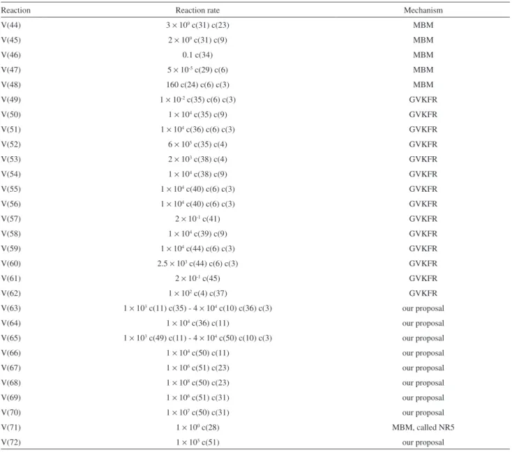
Table S2. continuation

Reaction Reaction rate Mechanism

V(44) 3 × 109 c(31) c(23) MBM

V(45) 2 × 109 c(31) c(9) MBM

V(46) 0.1 c(34) MBM

V(47) 5 × 10-5 c(29) c(6) MBM

V(48) 160 c(24) c(6) c(3) MBM

V(49) 1 × 10-2 _{c(35) c(6) c(3) GVKFR}

V(50) 1 × 104 c(35) c(9) GVKFR

V(51) 1 × 104 _{c(36) c(6) c(3) GVKFR}

V(52) 6 × 105 c(35) c(4) GVKFR

V(53) 2 × 103 _{c(38) c(4) GVKFR}

V(54) 1 × 104 _{c(38) c(9) GVKFR}

V(55) 1 × 104 c(40) c(6) c(3) GVKFR

V(56) 1 × 104 _{c(40) c(6) c(3) GVKFR}

V(57) 2 × 10-1 c(41) GVKFR

V(58) 1 × 104 c(39) c(9) GVKFR

V(59) 1 × 104 _{c(44) c(6) c(3) GVKFR}

V(60) 2.5 × 103 c(44) c(6) c(3) GVKFR

V(61) 2 × 10-1 _{c(45) GVKFR}

V(62) 1 × 102 _{c(4) c(37) GVKFR}

V(63) 1 × 103 c(11) c(35) - 4 × 104 c(10) c(36) c(3) our proposal

V(64) 1 × 104 _{c(36) c(11) our proposal}

V(65) 1 × 103 c(49) c(11) - 4 × 104 c(50) c(10) c(3) our proposal

V(66) 1 × 104 _{c(50) c(11) our proposal}

V(67) 1 × 106 _{c(51) c(23) our proposal}

V(68) 1 × 108 c(50) c(23) our proposal

V(69) 1 × 106 _{c(51) c(31) our proposal}

V(70) 1 × 107 c(50) c(31) our proposal

V(71) 1 × 100 c(28) MBM, called NR5

V(72) 1 × 105 _{c(51) our proposal}

All variables used in the computer program were double

precision, and the tolerance for the convergence of the

algorithm was set to 1 × 10

_{. Others tolerances were tested}

Source code

!Revisado septiembre 17 de 2013. Program BarridoFenol

Implicit none

DOUBLE PRECISION CFenol Integer contador

! Do contador=1,18,1

! If (contador .EQ. 1) then; CFenol=0D0; end if ! If (contador .EQ. 2) then; CFenol=5.347D-5; end if ! If (contador .EQ. 3) then; CFenol=1.337D-4; end if ! If (contador .EQ. 4) then; CFenol=2.673D-4; end if ! If (contador .EQ. 5) then; CFenol=5.347D-4; end if ! If (contador .EQ. 6) then; CFenol=1.069D-3; end if ! If (contador .EQ. 7) then; CFenol=1.337D-3; end if ! If (contador .EQ. 8) then; CFenol=1.604D-3; end if ! If (contador .EQ. 9) then; CFenol=1.871D-2; end if ! If (contador .EQ. 10) then; CFenol=2.272D-2; end if ! If (contador .EQ. 11) then; CFenol=2.673D-2; end if ! If (contador .EQ. 12) then; CFenol=3.074D-2; end if ! If (contador .EQ. 13) then; CFenol=3.476D-2; end if ! If (contador .EQ. 14) then; CFenol=3.877D-2; end if ! If (contador .EQ. 15) then; CFenol=4.278D-2; end if ! If (contador .EQ. 16) then; CFenol=4.679D-2; end if ! If (contador .EQ. 17) then; CFenol=5.347D-2; end if ! If (contador .EQ. 18) then; CFenol=1.069D-1; end if

contador=18 ! The variable “contador” must be change from 1 to 18 to choose one of the experimental concentrations of phenol used.

If (contador .EQ. 1) then; CFenol=0D0; end if If (contador .EQ. 2) then; CFenol=5.347D-5; end if If (contador .EQ. 3) then; CFenol=1.337D-4; end if If (contador .EQ. 4) then; CFenol=2.673D-4; end if If (contador .EQ. 5) then; CFenol=5.347D-4; end if If (contador .EQ. 6) then; CFenol=1.069D-3; end if If (contador .EQ. 7) then; CFenol=1.337D-3; end if If (contador .EQ. 8) then; CFenol=1.604D-3; end if If (contador .EQ. 9) then; CFenol=1.871D-2; end if If (contador .EQ. 10) then; CFenol=2.272D-2; end if If (contador .EQ. 11) then; CFenol=2.673D-2; end if If (contador .EQ. 12) then; CFenol=3.074D-2; end if If (contador .EQ. 13) then; CFenol=3.476D-2; end if If (contador .EQ. 14) then; CFenol=3.877D-2; end if If (contador .EQ. 15) then; CFenol=4.278D-2; end if If (contador .EQ. 16) then; CFenol=4.679D-2; end if If (contador .EQ. 17) then; CFenol=5.347D-2; end if If (contador .EQ. 18) then; CFenol=1.069D-1; end if write(*,*) “Contador = “,contador,”CFenol = “, CFenol ! call sleep(1)

call MBMReGVKFR(contador,CFenol) ! write(*,*) “CFenol = “, CFenol ! call sleep(1)

! End Do

end Program BarridoFenol

Subroutine MBMReGVKFR(contador,CFenol) Implicit none

EXTERNAL F, Jac

DOUBLE PRECISION ATOL, RWORK, RTOL, T, Tmax,TOUT,c, Delta,Hmax, +Max_step,CFenol

Integer neq,ITOL,ITASK,ISTATE,IOPT,LRW,LIW,MF,LPR,IWORK,I,contador DIMENSION c(51),RWORK(3100), IWORK(100)

character*19 graile

C write(*,20)

C 20 format(2x,’Archivo para los datos de integracion: ‘)

C read(*,15) graile

If (contador .LT. 10) then

write(ContadorArchivo1,’(I1)’) contador !convierte entero a caracter ! ContadorArchivo=trim(ContadorArchivo) !Quita los espacios en blanco

graile=”Ago-26-2013-”//trim(ContadorArchivo1)//”.txt”

else

write(ContadorArchivo2,’(I2)’) contador

graile=”Ago-26-2013-”//trim(ContadorArchivo2)//”.txt”

End if

C Aqui se especiica el número de ecuaciones diferenciales ODES

neq=51

C *** !Estos datos son los que debe leer la subrutina, o se le deben dar C WRITE(*,*) ‘Entre el tiempo total de la simulación: ‘

C READ(*,*) Tmax

C WRITE(*,*) ‘Entre el intervalo del tiempo: ‘ C READ(*,*) Delta

Tmax=2D6 !4D4 !4D5 !2D6 Delta=40D0

C Concentraciones Iniciales de cada especie C WRITE(*,*) ‘Entre la concentración inicial 1: ‘ C read(*,*) c(1)

C WRITE(*,*) ‘Entre la concentración inicial 2: ‘ C read(*,*) c(2)

c(1)=0.00000001 ! c(1)= Br-c(2)=0.0 ! c(2)= HOBr c(3)=1.29 ! c(3)= H+ c(4)=0.0 ! c(4)= Br2 c(5)=0.0 ! c(5)= HBrO2

c(6)=2.8896D-2 ! Concentraci≤n Ariel !MBM articulo concentraci≤n 0.15D0 ! c(6)=

BrO3-c(7)=0.0 ! c(7)= H2BrO2+ c(8)=0.0 ! c(8)= Br2O4 c(9)=0.0 ! c(9)= BrO2* c(10)=0.0 ! c(10)= Ce+3

c(11)=5.606D-4 ! Concentraci≤n Ariel !MBM articulo concentracion 3.56D-4 ! c(11)=

Ce+4

c(12)=0.0 ! c(12)= O2 c(13)=0.0 ! c(13)= BrMA c(14)=0.0 ! c(14)= BrMA* c(15)=0.0 ! c(15)= BrEETRA c(16)=0.0 ! c(16)= CO2 c(17)=0.0 ! c(17)= BrMA(enol) c(18)=0.0 ! c(18)= Br2MA c(19)=0.0 ! c(19)= BrMABrO2 c(20)=0.0 ! c(20)= OA c(21)=0.0 ! c(21)= BrTA c(22)=0.0 ! c(22)= MOA c(23)=0.0 ! c(23)= COOH* c(24)=0.0 ! c(24)= MA*

c(25)=2.6056D-2 ! Concentraci≤n Ariel !MBM articulo concentraci≤n 5D-2 ! c(25)=

MA

! *** Desde aquí se suman las reacciones del mecanismo GVKFR ***

c(35)=CFenol ! GVKFR: c(7)= R Fenol H2BrO2+ c(36)=0.0D0 ! GVKFR: c(8)= R* Fenol* = H-*Fenol=0 Br2O4 c(37)=0.0D0 ! GVKFR: c(10)= Rox1 HO-HFenol=0 Ce+3 c(38)=0.0D0 ! GVKFR: c(11)= RBr Br* Ce+4 c(39)=0.0D0 ! GVKFR: c(12)= RBr2 O=Fenol*-OH = *O-Fenol-OH O2 c(40)=0.0D0 ! GVKFR: c(13)= RBr* O=Fenol=0 BrMA c(41)=0.0D0 ! GVKFR: c(14)= R(BrOH) HO-Fenol-OH BrMA* c(42)=0.0D0 ! GVKFR: c(15)= Rox2 HO-Fenol-Br BrEETRA c(43)=0.0D0 ! GVKFR: c(16)= OQN (Fenol-O)2 CO2

c(44)=0.0D0 ! GVKFR: c(17)= RBr2* BrMA(enol) c(45)=0.0D0 ! GVKFR: c(18)= RBr(BrOH) Br2MA

c(46)=0.0D0 ! GVKFR: c(19)= Rox3 BrMABrO2 c(47)=0.0D0 ! GVKFR: c(20)= BrOQN OA c(48)=0.0D0 ! GVKFR: c(21)= Rox4 BrTA ! *** Las especies de las intereacciones

c(49)=0.0D0 ! Ariel: p-Hidroxyphenol

c(50)=0.0D0 ! Ariel: p-Hidroxyphenol radical c(51)=0.0D0 ! Ariel: p-Quinone

! write(*,*) “cs = “, (c(I), I=1, neq)

open(9, ile = graile, status=’replace’)

Hmax= 10D0 ! Maximun step size Max_step= 10000000D0

TOUT = 0D0 ITOL = 1

RTOL = 1.D-10 !tol : Error tolerance ATOL = 1.D-10 !wlimit : Error control limit ITASK = 1

ISTATE = 1 IOPT = 1 LRW = 3100 LIW = 100

MF = 22 !, por LSODE suministra el jacobiano full C Input options

Do lpr=5,10 rwork(lpr)=0 iwork(lpr)=0 End Do

C rwork(5)=H !h0 rwork(6)=Hmax

iwork(6)=Max_step

Do While (Tout .LE. Tmax) !Del ciclo de integracion DLSODE CALL DLSODE(F,NEQ,c,T,TOUT,ITOL,RTOL,ATOL,ITASK,ISTATE, + IOPT,RWORK,LRW,IWORK,LIW,Jac,MF)

! WRITE(6,32) T,c(1),c(2)

! 32 FORMAT(7H En T =,E12.4,7H c(1) =,E14.6,7H c(2) =,E14.6) WRITE(9,34) T,((c(I)), I=1, neq)

34 FORMAT(52(1PE13.5)) IF (ISTATE .LT. 0) Then WRITE(6,90)ISTATE

90 FORMAT(///22H ERROR HALT.. ISTATE =,I3)

close(9) STOP

End If

TOUT = TOUT + delta

End Do !in Del ciclo de integracion DLSODE **********************************

WRITE(6,60)IWORK(11),IWORK(12),IWORK(13)

60 FORMAT(/12H NO. STEPS =,I4,11H NO. F-S =,I4,11H NO. J-S =,I4)

END Subroutine MBMReGVKFR

C**************************************************** SUBROUTINE F (NEQ, T, c, YDOT)

DOUBLE PRECISION T, c, YDOT, V DIMENSION c(51), YDOT(51), V(72)

Integer especie

! *** Para controlar los posibles valores negativos de GVKFR R=c(7) y R*=c(8) Do especie=1, 51, 1

IF ( c(especie) < 1D-14 ) Then

c(especie)=0D0 !; write (*,*), ‘Se acabo el reactivo. c(7) =’, c(7) END IF

End Do

V(1)= 8d+9*c(1)*c(2)*c(3)-110*c(4)

V(2)= 2.9d+6*c(1)*c(5)*c(3)-2d-5*c(2)*c(2) V(3)= 0.6*c(1)*c(6)*c(3)*c(3)-3.2*c(2)*c(5) V(4)= 2d+6*c(5)*c(3)-1.0d+8*c(7)

V(5)= 1.7d+5*c(5)*c(7)

V(6)= 48*c(5)*c(6)*c(3)-3.2d+3*c(8) V(7)= 7.5d+4*c(8)-1.4d+9*c(9)*c(9)

V(8)= 6d+4*c(10)*c(9)*c(3)-1.3d+4*c(11)*c(5) V(9)= 6d-10*c(6)*c(6)*c(3)*c(3)

V(10)= 0.06*c(9)

V(11)= 0.1*c(13)*c(11)-400*c(14)*c(10)*c(3) V(12)= 1d+9*c(14)*c(14)

V(13)= 1.2d-2*c(13)-800*c(17) V(14)= 3.5d+6*c(17)*c(4) V(15)= 1.1d+6*c(17)*c(2) V(16)= 2d+9*c(14)*c(9) V(17)= 0.62*c(19) V(18)= 0.46*c(19) V(19)= 1.5*c(21)

V(20)= 7d+3*c(22)*c(11) V(21)= 28*c(20)*c(11) V(22)= 5d+9*c(23)*c(23) V(23)= 1d+7*c(23)*c(11)

V(24)= 0.6d+6*c(23)*c(13) V(25)= 3d+9*c(23)*c(14)

V(26)= 5d+9*c(23)*c(9)

V(27)= 0.23*c(25)*c(11)-2.2d+4*c(24)*c(10)*c(3) V(28)= 3.2d+9*c(24)*c(24)

V(29)= 2.6d-3*c(25)-180*c(27) V(30)= 2d+6*c(27)*c(4) V(31)= 6.7d+5*c(27)*c(2) V(32)= 5d+9*c(24)*c(9) V(33)= 0.55*c(28) V(34)= 1.0*c(28)

V(35)= 2d+9*c(24)*c(14) V(36)= 4d+9*c(24)*c(23)

V(37)= 0.66*c(29)*c(11)-1.7d+4*c(31)*c(10)*c(3) V(38)= 1d+9*c(31)*c(31)

V(39)= 2.3d-5*c(29)-1.5*c(33) V(40)= 3d+5*c(33)*c(4) V(41)= 2d+5*c(33)*c(2)

V(42)= 1d+9*c(31)*c(24) V(43)= 1d+9*c(31)*c(14)

V(44)= 3d+9*c(31)*c(23) V(45)= 2d+9*c(31)*c(9) V(46)= 0.1*c(34) V(47)= 5d-5*c(29)*c(6) V(48)= 160*c(24)*c(6)*c(3)

! *** Desde aquí se suman las velocidades del mecanismo GVKFR *** V(49)= 1D-2*c(35)*c(6)*c(3)

V(55)= 1D4*c(40)*c(6)*c(3) V(56)= 1D4*c(40)*c(6)*c(3) V(57)= 2D-1*c(41)

V(58)= 1D4*c(39)*c(9) V(59)= 1D4*c(44)*c(6)*c(3) V(60)= 2.5D3*c(44)*c(6)*c(3) V(61)= 2D-1*c(45)

V(62)= 1D2*c(4)*c(37)

! *** Estas reacciones se adiciona, digamos inter mecanismos *** ! Se usa el formato largo, propuesto por Ariel - Ver cuaderno. V(63)= 1D3*c(11)*c(35)-4D4*c(10)*c(36)*c(3)

V(64)= 1D4*c(36)*c(11)

V(65)= 1D3*c(49)*c(11)-4D4*c(50)*c(10)*c(3) V(66)= 1D4*c(50)*c(11)

V(67)= 1D6*c(51)*c(23) V(68)= 1D8*c(50)*c(23) V(69)= 1D6*c(51)*c(31) V(70)= 1D7*c(50)*c(31)

! *** NR5 Revisado en la web http://www.phy.bme.hu/deps/chem_ph/Research/BZ_Simulation/Ce4+.html

V(71)= 1D0*c(28)

! *** Se adiciona una reacci≤n de consumo de la quinona, para representar la desaparici≤n de esta y por tanto la desaparici≤n del ciclo que origina los “burst”.

V(72)= 1D5*c(51) C Br-

YDOT(1)=-V(1)-V(2)-V(3)+V(12)+V(14)+V(17)+V(19)+V(24)+V(30) ++V(35)+V(40)+V(52)+V(53)+V(57)+V(62)+V(71)

C HOBr

YDOT(2)=-V(1)+2*V(2)+V(3)+V(5)-V(15)+V(17)-V(31)+V(33)-V(41) C H+

YDOT(3)=-V(1)-V(2)-2*V(3)-V(4)+2*V(5)-V(6)-V(8)-2*V(9)+V(11) ++V(12)+V(14)+V(17)+V(19)+V(20)+V(21)+V(23)+V(24)+V(27)+V(30) ++V(35)+V(37)+V(40)-V(48)-V(49)-V(51)+V(52)+V(53)-V(55)-V(56) ++V(57)-V(59)-V(60)+V(61)+V(62)+V(63)+V(64)+V(65)+V(66)+V(71) c Br2

YDOT(4)=V(1)+0.5*V(10)-V(14)-V(30)-V(40)-V(52)-V(53)-V(62)

c HBrO2 YDOT(5)=-V(2)+V(3)-V(4)-V(5)-V(6)+V(8)+2*V(9)+V(18)+V(26)+V(34) ++V(46)+V(47)+V(50)+V(54)+V(58)

c BrO3-

YDOT(6)=-V(3)+V(5)-V(6)-2*V(9)-V(47)-V(48)-V(49)-V(51)-V(55) +-V(56)-V(59)-V(60)

c H2BrO2+ YDOT(7)=V(4)-V(5)

c Br2O4

YDOT(8)=V(6)-V(7)

c BrO2*

YDOT(9)=2*V(7)-V(8)-V(10)-V(16)-V(26)-V(32)-V(45)+V(48)+V(49) +-V(50)-V(54)+V(55)+V(56)-V(58)+V(59)+V(60)

c Ce+3

YDOT(10)=-V(8)+V(11)+V(20)+V(21)+V(23)+V(27)+V(37)+V(63)+V(64) ++V(65)+V(66)

c Ce+4

c O2

YDOT(12)=V(9)+V(10) !!!!Solo se acumula

c BrMA

YDOT(13)=-V(11)-V(13)-V(24)+V(25)+V(30)+V(31)

c BrMA*

YDOT(14)=V(11)-2*V(12)-V(16)-V(25)-V(35)-V(43)

c BrEETRA

YDOT(15)=V(12)+V(43) !!!!Solo se acumula

c CO2

YDOT(16)=V(12)+V(17)+V(21)+V(23)+V(24)+V(25)+V(26)+V(36)+V(38) ++V(43)+V(44)+V(67)+V(68)+V(71) !!!!Solo se acumula

c BrMA(enol)

YDOT(17)=V(13)-V(14)-V(15)

c Br2MA

YDOT(18)=V(14)+V(15) !!!!Solo se acumula

c BrMABrO2 YDOT(19)=V(16)-V(17)-V(18)

c OA

YDOT(20)=V(17)+V(20)-V(21)+V(22)+V(71)

c BrTA

YDOT(21)=V(18)-V(19)+V(40)+V(41)

c MOA

YDOT(22)=V(19)-V(20)+V(33)+V(46)+V(47)+V(69)+V(70)

c COOH*

YDOT(23)=V(20)+V(21)-2D0*V(22)-V(23)-V(24)-V(25)-V(26)-V(36) +-V(44)-V(67)-V(68)

c MA*

YDOT(24)=V(24)+V(27)-2*V(28)-V(32)-V(35)-V(36)-V(42)-V(48)

c MA

YDOT(25)=-V(27)-V(29)+V(36)

c ETA

YDOT(26)=V(28) !!!Solo se acumula

c MA(enol)

YDOT(27)=V(29)-V(30)-V(31) c MABrO2

YDOT(28)=V(32)-V(33)-V(34)-V(71) c TA

YDOT(29)=V(34)-V(37)-V(39)+V(44)-V(47)

c EETA

YDOT(30)=V(35)+V(42) !!!!Solo se acumula c TA*

YDOT(31)=V(37)-2*V(38)-V(42)-V(43)-V(44)-V(45)-V(69)-V(70)

c EEHTRA

YDOT(32)=V(38) !!!!Solo se acumula

c TA(enol)

c TABrO2 YDOT(34)=V(45)-V(46)

! *** Desde aquφ se suman las EDOs de las especies del mecanismo GVKFR

! R Fenol H2BrO2+ YDOT(35)=-V(49)-V(50)-V(52)-V(63)

! R* Fenol* = H-*Fenol=0 Br2O4 YDOT(36)=V(49)+V(50)-V(51)+V(63)-V(64)

! Rox1 HO-HFenol=0 Ce+3 YDOT(37)=V(51)-V(62)

! RBr Br* Ce+4 YDOT(38)=V(52)-V(53)-v(54)

! RBr2 O=Fenol*-OH = *O-Fenol-OH O2 YDOT(39)=V(53)-V(58)

! RBr* O=Fenol=0 BrMA YDOT(40)=V(54)-V(55)-V(56)

! R(BrOH) HO-Fenol-OH BrMA* YDOT(41)=V(55)-V(57)

! Rox2 HO-Fenol-Br BrEETRA YDOT(42)=V(56) !!!!Solo se acumula

! OQN (Fenol-O)2 CO2 YDOT(43)=V(57) !!!!Solo se acumula

! RBr2*

YDOT(44)=V(58)-V(59)-V(60) ! RBr(BrOH)

YDOT(45)=V(59)-V(61) ! Rox3

YDOT(46)=V(60) !!!!Solo se acumula ! BrOQN

YDOT(47)=V(61) !!!!Solo se acumula ! Rox4

YDOT(48)=V(62) !!!!Solo se acumula ! ROH - p-Hidroxifenol - Especie nueva YDOT(49)=V(64)-V(65)+V(68)+V(70)

! p-Hidroxifenol Radical - Especie nueva YDOT(50)=V(65)-V(66)+V(67)-V(68)+V(69)-V(70) ! p-Quinona - Especie nueva

YDOT(51)=V(66)-V(67)-V(69)-V(72) END SUBROUTINE !F

SUBROUTINE JAC END SUBROUTINE JAC

C*********************************************************************************** *DECK DLSODE

SUBROUTINE DLSODE (F, NEQ, Y, T, TOUT, ITOL, RTOL, ATOL, ITASK, 1 ISTATE, IOPT, RWORK, LRW, IWORK, LIW, JAC, MF) C***BEGIN PROLOGUE DLSODE

C***PURPOSE Livermore solver for ordinary differential equations. C DLSODE solves the initial-value problem for stiff or

C nonstiff systems of irst-order ODE’s, C dy/dt = f(t,y), or, in component form,

C dy(i)/dt = f(i) = f(i,t,y(1),y(2),...,y(N)), i=1,...,N.

C***TYPE DOUBLE PRECISION (SLSODE-S, DLSODE-D)

C***KEYWORDS ORDINARY DIFFERENTIAL EQUATIONS, INITIAL VALUE PROBLEM, C STIFF, NONSTIFF

C***AUTHOR Hindmarsh, Alan C., (LLNL)

C Computing and Mathematics Research Div., L-316 C Lawrence Livermore National Laboratory

C Livermore, CA 94550. C***DESCRIPTION

C

C NOTE: The DLSODE solver is not re-entrant, and so is usable on C the Cray multi-processor machines only if it is not used C in a multi-tasking environment.

C If re-entrancy is required, use NLSODE instead. C

C The formats of the DLSODE and NLSODE writeups differ from C those of the other MATHLIB routines.

C

C The “Usage” and “Arguments” sections treat only a subset of C available options, in condensed fashion. The options C covered and the information supplied will support most C standard uses of DLSODE.

C

C For more sophisticated uses, full details on all options are C given in the concluding section, headed “Long Description.” C A synopsis of the DLSODE Long Description is provided at the C beginning of that section; general topics covered are: C - Elements of the call sequence; optional input and output C - Optional supplemental routines in the DLSODE package C - internal COMMON block

C

C *Usage:

C Communication between the user and the DLSODE package, for normal C situations, is summarized here. This summary describes a subset C of the available options. See “Long Description” for complete C details, including optional communication, nonstandard options, C and instructions for special situations.

C

C A sample program is given in the “Examples” section. C

C Refer to the argument descriptions for the deinitions of the

C quantities that appear in the following sample declarations. C

C For MF = 10,

C PARAMETER (LRW = 20 + 16*NEQ, LIW = 20) C For MF = 21 or 22,

C PARAMETER (LRW = 22 + 9*NEQ + NEQ**2, LIW = 20 + NEQ) C For MF = 24 or 25,

C PARAMETER (LRW = 22 + 10*NEQ + (2*ML+MU)*NEQ,

C * LIW = 20 + NEQ) C

C EXTERNAL F, JAC

C INTEGER NEQ, ITOL, ITASK, ISTATE, IOPT, LRW, IWORK(LIW), C * LIW, MF

C DOUBLE PRECISION Y(NEQ), T, TOUT, RTOL, ATOL(ntol), RWORK(LRW) C

C CALL DLSODE (F, NEQ, Y, T, TOUT, ITOL, RTOL, ATOL, ITASK, C * ISTATE, IOPT, RWORK, LRW, IWORK, LIW, JAC, MF) C

C *Arguments:

C F :EXT Name of subroutine for right-hand-side vector f. C This name must be declared EXTERNAL in calling C program. The form of F must be:

C

C SUBROUTINE F (NEQ, T, Y, YDOT) C INTEGER NEQ

C The inputs are NEQ, T, Y. F is to set C

C YDOT(i) = f(i,T,Y(1),Y(2),...,Y(NEQ)),

C i = 1, ..., NEQ . C

C NEQ :IN Number of irst-order ODE’s.

C

C Y :INOUT Array of values of the y(t) vector, of length NEQ.

C Input: For the irst call, Y should contain the

C values of y(t) at t = T. (Y is an input C variable only if ISTATE = 1.)

C Output: On return, Y will contain the values at the C new t-value.

C

C T :INOUT Value of the independent variable. On return it C will be the current value of t (normally TOUT). C

C TOUT :IN Next point where output is desired (.NE. T). C

C ITOL :IN 1 or 2 according as ATOL (below) is a scalar or C an array.

C

C RTOL :IN Relative tolerance parameter (scalar). C

C ATOL :IN Absolute tolerance parameter (scalar or array). C If ITOL = 1, ATOL need not be dimensioned.

C If ITOL = 2, ATOL must be dimensioned at least NEQ. C

C The estimated local error in Y(i) will be controlled C so as to be roughly less (in magnitude) than

C

C EWT(i) = RTOL*ABS(Y(i)) + ATOL if ITOL = 1, or C EWT(i) = RTOL*ABS(Y(i)) + ATOL(i) if ITOL = 2. C

C Thus the local error test passes if, in each C component, either the absolute error is less than C ATOL (or ATOL(i)), or the relative error is less C than RTOL.

C

C Use RTOL = 0.0 for pure absolute error control, and C use ATOL = 0.0 (or ATOL(i) = 0.0) for pure relative C error control. Caution: Actual (global) errors may C exceed these local tolerances, so choose them C conservatively.

C

C ITASK :IN Flag indicating the task DLSODE is to perform. C Use ITASK = 1 for normal computation of output C values of y at t = TOUT.

C

C ISTATE:INOUT Index used for input and output to specify the state C of the calculation.

C Input:

C 1 This is the irst call for a problem.

C 2 This is a subsequent call. C Output:

C 2 DLSODE was successful (otherwise, negative).

C Note that ISTATE need not be modiied after a

C successful return.

C -1 Excess work done on this call (perhaps wrong C MF).

C -2 Excess accuracy requested (tolerances too C small).

C -3 Illegal input detected (see printed message). C -4 Repeated error test failures (check all C inputs).

C tolerances).

C -6 Error weight became zero during problem C (solution component i vanished, and ATOL or C ATOL(i) = 0.).

C

C IOPT :IN Flag indicating whether optional inputs are used: C 0 No.

C 1 Yes. (See “Optional inputs” under “Long C Description,” Part 1.)

C

C RWORK :WORK Real work array of length at least:

C 20 + 16*NEQ for MF = 10, C 22 + 9*NEQ + NEQ**2 for MF = 21 or 22, C 22 + 10*NEQ + (2*ML + MU)*NEQ for MF = 24 or 25. C

C LRW :IN Declared length of RWORK (in user’s DIMENSION C statement).

C

C IWORK :WORK Integer work array of length at least: C 20 for MF = 10,

C 20 + NEQ for MF = 21, 22, 24, or 25. C

C If MF = 24 or 25, input in IWORK(1),IWORK(2) the C lower and upper Jacobian half-bandwidths ML,MU. C

C On return, IWORK contains information that may be C of interest to the user:

C

C Name Location Meaning

C --- --- ---C NST IWORK(11) Number of steps taken for the problem so C far.

C NFE IWORK(12) Number of f evaluations for the problem C so far.

C NJE IWORK(13) Number of Jacobian evaluations (and of C matrix LU decompositions) for the problem C so far.

C NQU IWORK(14) Method order last used (successfully). C LENRW IWORK(17) Length of RWORK actually required. This

C is deined on normal returns and on an C illegal input return for insuficient

C storage.

C LENIW IWORK(18) Length of IWORK actually required. This

C is deined on normal returns and on an C illegal input return for insuficient

C storage. C

C LIW :IN Declared length of IWORK (in user’s DIMENSION C statement).

C

C JAC :EXT Name of subroutine for Jacobian matrix (MF = C 21 or 24). If used, this name must be declared C EXTERNAL in calling program. If not used, pass a C dummy name. The form of JAC must be:

C

C SUBROUTINE JAC (NEQ, T, Y, ML, MU, PD, NROWPD) C INTEGER NEQ, ML, MU, NROWPD

C DOUBLE PRECISION T, Y(NEQ), PD(NROWPD,NEQ) C

C See item c, under “Description” below for more C information about JAC.

C

C MF :IN Method lag. Standard values are:

C 10 Nonstiff (Adams) method, no Jacobian used. C 21 Stiff (BDF) method, user-supplied full Jacobian. C 22 Stiff method, internally generated full

C 24 Stiff method, user-supplied banded Jacobian. C 25 Stiff method, internally generated banded C Jacobian.

C

C *Description:

C DLSODE solves the initial value problem for stiff or nonstiff

C systems of irst-order ODE’s,

C

C dy/dt = f(t,y) ,

C

C or, in component form, C

C dy(i)/dt = f(i) = f(i,t,y(1),y(2),...,y(NEQ))

C (i = 1, ..., NEQ) . C

C DLSODE is a package based on the GEAR and GEARB packages, and on C the October 23, 1978, version of the tentative ODEPACK user

C interface standard, with minor modiications.

C

C The steps in solving such a problem are as follows. C

C a. First write a subroutine of the form C

C SUBROUTINE F (NEQ, T, Y, YDOT) C INTEGER NEQ

C DOUBLE PRECISION T, Y(NEQ), YDOT(NEQ) C

C which supplies the vector function f by loading YDOT(i) with C f(i).

C

C b. Next determine (or guess) whether or not the problem is stiff.

C Stiffness occurs when the Jacobian matrix df/dy has an

C eigenvalue whose real part is negative and large in magnitude C compared to the reciprocal of the t span of interest. If the

C problem is nonstiff, use method lag MF = 10. If it is stiff,

C there are four standard choices for MF, and DLSODE requires the C Jacobian matrix in some form. This matrix is regarded either C as full (MF = 21 or 22), or banded (MF = 24 or 25). In the C banded case, DLSODE requires two half-bandwidth parameters ML C and MU. These are, respectively, the widths of the lower and C upper parts of the band, excluding the main diagonal. Thus the C band consists of the locations (i,j) with

C

C i - ML <= j <= i + MU , C

C and the full bandwidth is ML + MU + 1 . C

C c. If the problem is stiff, you are encouraged to supply the C Jacobian directly (MF = 21 or 24), but if this is not feasible, C DLSODE will compute it internally by difference quotients (MF = C 22 or 25). If you are supplying the Jacobian, write a

C subroutine of the form C

C SUBROUTINE JAC (NEQ, T, Y, ML, MU, PD, NROWPD) C INTEGER NEQ, ML, MU, NRWOPD

C DOUBLE PRECISION Y, Y(NEQ), PD(NROWPD,NEQ) C

C which provides df/dy by loading PD as follows:

C - For a full Jacobian (MF = 21), load PD(i,j) with df(i)/dy(j),

C the partial derivative of f(i) with respect to y(j). (Ignore C the ML and MU arguments in this case.)

C - For a banded Jacobian (MF = 24), load PD(i-j+MU+1,j) with

C df(i)/dy(j); i.e., load the diagonal lines of df/dy into the

C rows of PD from the top down.

C - In either case, only nonzero elements need be loaded. C

C point at which answers are desired. This should also provide C for possible use of logical unit 6 for output of error messages C by DLSODE.

C

C Before the irst call to DLSODE, set ISTATE = 1, set Y and T to C the initial values, and set TOUT to the irst output point. To

C continue the integration after a successful return, simply C reset TOUT and call DLSODE again. No other parameters need be C reset.

C

C *Examples:

C The following is a simple example problem, with the coding needed C for its solution by DLSODE. The problem is from chemical kinetics, C and consists of the following three rate equations:

C

C dy1/dt = -.04*y1 + 1.E4*y2*y3

C dy2/dt = .04*y1 - 1.E4*y2*y3 - 3.E7*y2**2 C dy3/dt = 3.E7*y2**2

C

C on the interval from t = 0.0 to t = 4.E10, with initial conditions C y1 = 1.0, y2 = y3 = 0. The problem is stiff.

C

C The following coding solves this problem with DLSODE, using C MF = 21 and printing results at t = .4, 4., ..., 4.E10. It uses C ITOL = 2 and ATOL much smaller for y2 than for y1 or y3 because y2 C has much smaller values. At the end of the run, statistical C quantities of interest are printed.

C

C EXTERNAL FEX, JEX

C INTEGER IOPT, IOUT, ISTATE, ITASK, ITOL, IWORK(23), LIW, LRW, C * MF, NEQ

C DOUBLE PRECISION ATOL(3), RTOL, RWORK(58), T, TOUT, Y(3) C NEQ = 3

C Y(1) = 1.D0 C Y(2) = 0.D0 C Y(3) = 0.D0 C T = 0.D0 C TOUT = .4D0 C ITOL = 2 C RTOL = 1.D-4 C ATOL(1) = 1.D-6 C ATOL(2) = 1.D-10 C ATOL(3) = 1.D-6 C ITASK = 1 C ISTATE = 1 C IOPT = 0 C LRW = 58 C LIW = 23 C MF = 21

C DO 40 IOUT = 1,12

C CALL DLSODE (FEX, NEQ, Y, T, TOUT, ITOL, RTOL, ATOL, ITASK, C * ISTATE, IOPT, RWORK, LRW, IWORK, LIW, JEX, MF) C WRITE(6,20) T, Y(1), Y(2), Y(3)

C 20 FORMAT(‘ At t =’,D12.4,’ y =’,3D14.6) C IF (ISTATE .LT. 0) GO TO 80

C 40 TOUT = TOUT*10.D0

C WRITE(6,60) IWORK(11), IWORK(12), IWORK(13)

C 60 FORMAT(/’ No. steps =’,i4,’, No. f-s =’,i4,’, No. J-s =’,i4)

C STOP

C 80 WRITE(6,90) ISTATE

C 90 FORMAT(///’ Error halt.. ISTATE =’,I3)

C STOP C END C

C SUBROUTINE FEX (NEQ, T, Y, YDOT) C INTEGER NEQ

C YDOT(1) = -.04D0*Y(1) + 1.D4*Y(2)*Y(3) C YDOT(3) = 3.D7*Y(2)*Y(2)

C YDOT(2) = -YDOT(1) - YDOT(3) C RETURN

C END C

C SUBROUTINE JEX (NEQ, T, Y, ML, MU, PD, NRPD) C INTEGER NEQ, ML, MU, NRPD

C DOUBLE PRECISION T, Y(3), PD(NRPD,3) C PD(1,1) = -.04D0

C PD(1,2) = 1.D4*Y(3) C PD(1,3) = 1.D4*Y(2) C PD(2,1) = .04D0 C PD(2,3) = -PD(1,3) C PD(3,2) = 6.D7*Y(2)

C PD(2,2) = -PD(1,2) - PD(3,2) C RETURN

C END C

C The output from this program (on a Cray-1 in single precision) C is as follows.

C

C At t = 4.0000e-01 y = 9.851726e-01 3.386406e-05 1.479357e-02 C At t = 4.0000e+00 y = 9.055142e-01 2.240418e-05 9.446344e-02 C At t = 4.0000e+01 y = 7.158050e-01 9.184616e-06 2.841858e-01 C At t = 4.0000e+02 y = 4.504846e-01 3.222434e-06 5.495122e-01 C At t = 4.0000e+03 y = 1.831701e-01 8.940379e-07 8.168290e-01 C At t = 4.0000e+04 y = 3.897016e-02 1.621193e-07 9.610297e-01 C At t = 4.0000e+05 y = 4.935213e-03 1.983756e-08 9.950648e-01 C At t = 4.0000e+06 y = 5.159269e-04 2.064759e-09 9.994841e-01 C At t = 4.0000e+07 y = 5.306413e-05 2.122677e-10 9.999469e-01 C At t = 4.0000e+08 y = 5.494530e-06 2.197825e-11 9.999945e-01 C At t = 4.0000e+09 y = 5.129458e-07 2.051784e-12 9.999995e-01 C At t = 4.0000e+10 y = -7.170603e-08 -2.868241e-13 1.000000e+00 C

C No. steps = 330, No. f-s = 405, No. J-s = 69 C

C *Accuracy:

C The accuracy of the solution depends on the choice of tolerances C RTOL and ATOL. Actual (global) errors may exceed these local C tolerances, so choose them conservatively.

C

C *Cautions:

C The work arrays should not be altered between calls to DLSODE for C the same problem, except possibly for the conditional and optional C inputs.

C

C *Portability:

C Since NEQ is dimensioned inside DLSODE, some compilers may object C to a call to DLSODE with NEQ a scalar variable. In this event, C use DIMENSION NEQ(1). Similar remarks apply to RTOL and ATOL. C

C Note to Cray users:

C For maximum eficiency, use the CFT77 compiler. Appropriate

C compiler optimization directives have been inserted for CFT77 C (but not CIVIC).

C

C NOTICE: If moving the DLSODE source code to other systems, C contact the author for notes on nonstandard Fortran usage, C COMMON block, and other installation details.

C

C *Reference:

C Alan C. Hindmarsh, “ODEPACK, a systematized collection of ODE

C solvers,” in Scientiic Computing, R. S. Stepleman, et al., Eds.

C (North-Holland, Amsterdam, 1983), pp. 55-64. C

C The following complete description of the user interface to C DLSODE consists of four parts:

C

C 1. The call sequence to subroutine DLSODE, which is a driver C routine for the solver. This includes descriptions of both C the call sequence arguments and user-supplied routines. C Following these descriptions is a description of optional C inputs available through the call sequence, and then a C description of optional outputs in the work arrays. C

C 2. Descriptions of other routines in the DLSODE package that may C be (optionally) called by the user. These provide the ability C to alter error message handling, save and restore the internal

C COMMON, and obtain speciied derivatives of the solution y(t).

C

C 3. Descriptions of COMMON block to be declared in overlay or C similar environments, or to be saved when doing an interrupt C of the problem and continued solution later.

C

C 4. Description of two routines in the DLSODE package, either of C which the user may replace with his own version, if desired. C These relate to the measurement of errors.

C C

C Part 1. Call Sequence C ---C

C Arguments C

---C The call sequence parameters used for input only are C

C F, NEQ, TOUT, ITOL, RTOL, ATOL, ITASK, IOPT, LRW, LIW, JAC, MF, C

C and those used for both input and output are C

C Y, T, ISTATE. C

C The work arrays RWORK and IWORK are also used for conditional and C optional inputs and optional outputs. (The term output here C refers to the return from subroutine DLSODE to the user’s calling C program.)

C

C The legality of input parameters will be thoroughly checked on the C initial call for the problem, but not checked thereafter unless a

C change in input parameters is lagged by ISTATE = 3 on input.

C

C The descriptions of the call arguments are as follows. C

C F The name of the user-supplied subroutine deining the ODE C system. The system must be put in the irst-order form C dy/dt = f(t,y), where f is a vector-valued function of

C the scalar t and the vector y. Subroutine F is to compute C the function f. It is to have the form

C

C SUBROUTINE F (NEQ, T, Y, YDOT) C DOUBLE PRECISION Y(NEQ), YDOT(NEQ) C

C where NEQ, T, and Y are input, and the array YDOT = C f(T,Y) is output. Y and YDOT are arrays of length NEQ. C Subroutine F should not alter Y(1),...,Y(NEQ). F must be C declared EXTERNAL in the calling program.

C

C Subroutine F may access user-deined quantities in C NEQ(2),... and/or in Y(NEQ(1)+1),..., if NEQ is an array C (dimensioned in F) and/or Y has length exceeding NEQ(1).

C If quantities computed in the F routine are needed C externally to DLSODE, an extra call to F should be made C for this purpose, for consistent and accurate results.

C If only the derivative dy/dt is needed, use DINTDY

C instead. C

C NEQ The size of the ODE system (number of irst-order

C ordinary differential equations). Used only for input. C NEQ may be decreased, but not increased, during the C problem. If NEQ is decreased (with ISTATE = 3 on input), C the remaining components of Y should be left undisturbed,

C if these are to be accessed in F and/or JAC.

C

C Normally, NEQ is a scalar, and it is generally referred C to as a scalar in this user interface description. C However, NEQ may be an array, with NEQ(1) set to the C system size. (The DLSODE package accesses only NEQ(1).) C In either case, this parameter is passed as the NEQ C argument in all calls to F and JAC. Hence, if it is an C array, locations NEQ(2),... may be used to store other

C integer data and pass it to F and/or JAC. Subroutines C F and/or JAC must include NEQ in a DIMENSION statement

C in that case. C

C Y A real array for the vector of dependent variables, of C length NEQ or more. Used for both input and output on

C the irst call (ISTATE = 1), and only for output on C other calls. On the irst call, Y must contain the

C vector of initial values. On output, Y contains the C computed solution vector, evaluated at T. If desired, C the Y array may be used for other purposes between C calls to the solver.

C

C This array is passed as the Y argument in all calls to F C and JAC. Hence its length may exceed NEQ, and locations C Y(NEQ+1),... may be used to store other real data and

C pass it to F and/or JAC. (The DLSODE package accesses

C only Y(1),...,Y(NEQ).) C

C T The independent variable. On input, T is used only on

C the irst call, as the initial point of the integration.

C On output, after each call, T is the value at which a C computed solution Y is evaluated (usually the same as C TOUT). On an error return, T is the farthest point C reached.

C

C TOUT The next value of T at which a computed solution is C desired. Used only for input.

C

C When starting the problem (ISTATE = 1), TOUT may be equal C to T for one call, then should not equal T for the next C call. For the initial T, an input value of TOUT .NE. T C is used in order to determine the direction of the C integration (i.e., the algebraic sign of the step sizes) C and the rough scale of the problem. Integration in C either direction (forward or backward in T) is permitted. C

C If ITASK = 2 or 5 (one-step modes), TOUT is ignored

C after the irst call (i.e., the irst call with

C TOUT .NE. T). Otherwise, TOUT is required on every call. C

C If ITASK = 1, 3, or 4, the values of TOUT need not be C monotone, but a value of TOUT which backs up is limited C to the current internal T interval, whose endpoints are C TCUR - HU and TCUR. (See “Optional Outputs” below for C TCUR and HU.)