Abstract— The most appropriate prioritization method is still one of the unsettled issues of the Analytic Hierarchy Process, although many studies have been made and applied. Interestingly, many transportation evaluation and selection models using AHP apply only Saaty’s Eigenvector method. Many theoretical studies have found that this method may produce rank reversals and have proposed various prioritization methods as alternatives. Some methods have been proved to be superior to the Eigenvector method. However, a literature review shows that these methods seem not to attract the attention of researchers in this research area. In this paper, a Prioritization Operator Recommendation Model is proposed to address this issue. Eight important prioritization methods are reviewed. A Mixed Prioritization Operators model is developed to select a vector which has the most appropriate prioritization operators for generic evaluation and selection problems in transportation. To verify this new model, a case study is revised using the proposed model. The contribution is that MPOs are useful for solving prioritization problems in the AHP.
Index Terms—, Analytic Hierarchy Process, Multi Criteria
Decision Making, Rank reversal, Transportation Selection
I. INTRODUCTION
In Multiple Criteria Decision Making, the criteria are usually classified as being of two kinds: quantitative criteria which can be measured by number such as amount of time, labor, cost, and price; qualitative criteria such as quality and qualitative weights which cannot be objectively and directly determined, but which are usually determined by subjective judgment. The Analytic Hierarchy Process [13] is the popular tool for the subjective judgment of the qualitative data. In the transportation evaluation and selection problems, the AHP can be applied to the qualitative analysis.
For the evaluation issue, AHP can be used for determining the weights of multi-criteria, which are further incorporated into other models. For example, Tanadtang et al. [18] adopted AHP to measure the weights of criteria for evaluating transportation demand management (TDM) alternatives. Sohn[16] proposed a model for the Seoul Metropolitan Government to eliminate some useless overpasses among 22
Kevin Kam Fung Yuen is with Department of Industrial and Systems Engineering, The Hong Kong Polytechnic University, Hung Hom, KLN, Hong Kong (e-mail:[email protected];
existing overpasses, and the weights of this model adopted AHP methodology. In selection problems, Saaty [12, 15] proposed applying AHP in different scenarios in transport planning. Ferrari [7] proposed a method for choosing from among alternative transportation projects. Kulak and Kahraman [9] proposed a crisp AHP model and a fuzzy AHP model to solve transportation company selection problems. The methodology of a fuzzy AHP model also can be found in [21-23]. A Crisp AHP is a special case of a fuzzy AHP.
The AHP includes three major processes: assessment, prioritization, and synthesis. In the assessment, verbal judgments are given by decision makers for pairwise comparisons. The verbal judgment is usually on a 9 point verbal scale represented by numbers: 1 for equal importance, 2 for weak importance, and finally 9 for extreme importance. For pairwise comparisons, aij is a numeric point to estimate
the relative importance of object i over object j, and A
aij ,1
0 aij aji
, ,i j1, 2,,n is a pairwise comparison matrix. Thus a pairwise comparison matrix is also called a reciprocal matrix. The reciprocal matrices of all assessments are formed by transforming the linguistic labels to numerical values. In the prioritization process, a local priority vector
1, , n
W w w ,
ni1wi 1 is generated from a reciprocalmatrix A by a Prioritization Operator (PO), i.e.
:
PO AW . In the synthesis stage, these local priority vectors W’s are aggregated as a global priority vector
1, , n
V v v by an aggregation operator Agg:
W V. These processes are likely to induce three fundamental problems: (i) selection of numerical scales in stage one; (ii) selection of prioritization operators (or methods) in stage two, and (iii) selection of aggregation operators in stage three. These three problems probably create rank reversals. Problem (i) is addressed by [19,24]. This research focuses on the solution of rank reversals due to problem (ii) using the most appropriate approximate prioritization operator.Although there are many POs (illustrated in section 2), actually the best prioritization operator relies on the content of a pairwise matrix, and none of prioritization methods performs better than the others in every inconsistent case. The application in this study and Refs.[10,17,20] also verify this issue. Thus, it is most appropriate to propose a framework to select the most appropriate prioritization operator for each reciprocal matrix among sufficient PO candidates with an objective measurement method. This study proposes a Mixed Prioritization Operators strategy for this measurement
On Limitations of the Prioritization Methods in
Analytic Hierarchy Process: A Study of
Transportation Selection Problems
method.
The structure of this article is as follows: Section 2 reviews the Prioritization Operators. Section 3 proposes a measurement model to measure the POs, and Mixed POs are proposed. Section 4 revises the application adopted from Kulak and Kahramna [9] using Mix POs strategy. In section 5 a conclusion to this paper is drawn.
II. PRIORITIZATIONOPERATORS
Eight essential prioritization operators are reviewed as follows:
2.1 Eigenvector(EV)
The Eigenvector operator for intuitive justification is proposed by Saaty[13]. EV derives the principal eigenvector
max
of A as the priority vector w by solving following Eigen system.
max
Aw w, and
1 1
n i iw
(1)A is consistent if and only ifmax n, and is not consistent if and only if max n where maxn.
The Normalization operator was introduced in Saaty[13]. The following methods (2.2-2.5) are named according to their calculation steps since Saaty[13] has not given them appropriate names.
2.2 Normalization of the Row Sum (NRS)
NRS sums up the elements in each row and normalizes by dividing each sum by the total of all the sums, thus the results now add up to unity. NRS has the form:
1
'i n ij 1, 2, ,
j
a
a i n1
'
1, 2, , ' i i n i i a
w i n
a
(2)2.3 Normalization of Reciprocals of Column Sum (NRCS) NRCS takes the sum of the elements in each column, forms the reciprocals of these sums, and then normalizes so that these numbers add up to unity, e.g. to divide each reciprocal by the sum of the reciprocals. It is in this form:
1
1
'i n j 1, 2, ,
ij i a n a
1 '1, 2, , ' i i n i i a
w i n
a
(3)2.4 Arithmetic Mean of Normalized Columns (AMNC) AMNC was also called the Additive Normalization method in [10]. The new name is relatively clear, in that it describes its calculation process. Each element in A is divided by the sum of each column in A, and then the mean of each row is taken as the priority wi. It has the form:
1
'ij nij , 1, 2, ,
ij i
a
a i j n
a
, and1
1
' 1, 2, , n
i j ij
w a i n
n
(4)The AHP applications use this method due to the simplicity of its calculation process.
2.5 Normalization of Geometric Means of Rows (NGMR) / Logarithm Least Squares (LLS)
NHMR multiplies the n elements in each row and takes the nth root, and then normalizes so that these numbers add up to unity. It is in the form:
1/ 1
1
' , 1, 2, ,
'
, 1, 2, , '
n n
i j ij
i
i n
i i
w a i n
w
w i n
w
(5)Although it is more complex than other three normalization methods, it is recommended by some authors [e.g. 1, 4] since this method produces the same result as LLS, which is in the form:
2
1 1
1
Min
Subject to 1, 0, 1, 2, ,
n n i ij i j j n i i i w a w
w w i n
(6)Saaty and Vargas [14] made comparisons among EV, LLS, and DLS. EV and LLS were discussed previously. DLS is as follows.
2.6 Direct Least Squares / Weighted Least Squares (DLS/WLS)
This method is used to minimize the sum of errors of the differences between the judgments and their derived values. The Direct Least Squares, which was proposed in [5], is in the form:
2
1 1
1
Min
Subject to 1, 0, 1, 2, ,
n n i ij i j j n i i i w a w
w w i n
(7)The above non-linear optimization problem has no special tractable form or closed form and thus is very difficult to be solved [5]. For efficient computation with a closed form, Chu at el. [5] modified the objective function and proposed the Weighted Least Squares (WLS)in the form:
21 1
1
Min
Subject to 1, 0, 1, 2, ,
n n
i ij j
i j
n
i i
i
w a w
w w i n
(8)2.7 Fuzzy Programming (FP)
The FP is proposed by Mikehailov [11], which has the form:
1
max
Subject to ,
, 1, 2, , , 1 0
1, 0, 1, 2, , T
j j j
T
j j j
n
i i
i
d R W d
d R W d j m
w w j n
m n
j ij
R R a is the row vector. The values of the left and right tolerance parameters dj
and dj
represent the admissible interval of approximate satisfaction of the crisp equality T 0
j
R W . The measure of intersection of is a natural consistency index of the FP. Its value however depends on the tolerance parameters. For the practical implementation of the FP, it is reasonable that all these parameters be set equal to each other. The limitation of this method is that parameters dj
and dj
are undetermined in [11]. This leads to infinite candidate values for them. [11] set
1
j j
dd in his example.
2.8 Goal Programming (GP)
Bryson [2] proposed a goal programming operator (GP) with the form:
1
Min ln = ln ln
Subject to ln ln ln ln ln , ,
n n
ij ij
i j i
i j ij ij ij
w w a i j IJ
where IJ
i j, :1 i j n
; lnij
and lnij
are
non-negative. (10)
Ideally the objective value should be 0 when
lnij lnij 0
, i.e. ij ij 1
.
When priorities are used as rank, the exact values of the rank are not so important so long as the ranks are preserved. However, when the priorities are used as weights, not only is the rank preservation important, but also the exact values of the priorities of the weights are essential. A little variation in the value of the priorities might possibly result in a different solution. When there are many prioritization operators, it is necessary to develop a measurement model to determine which operator is the most appropriate one. This is addressed in the next section.
III. MEASUREMENTMODELANDMIXED PRIORITIZATIONOPERATORSSTRATEGY The measurement models measure the validity of the prioritization operators. Thus they can be used for the comparing different POs. Two variance methods are reviewed and a new variance model, which is used for Mix POs strategy, is developed.
To measure the distribution of the variance, one approach is to use Root Mean Square Variance which has the form
2 1 1 1 , n n i iji j j
w
RMSV A W a
n n w
(11)A is a pairwise matrix
aij, W is a priorities vector of a prioritization operator, and w wi, j W
W1,,WK
W .If 1
n n is taken out, the new form is Euclidean Distance,
which was used by [8]. For easier interpretation of the result, it is more appropriate to use the average of the value. Thus RMSV is preferred.
However, a limitation of RMSV is that the weights for the penalty are not justified. For example, the penalty of the
condition
& 1& i
i j ij ij
j
w
w w a a True w
is not the
same as the one of the condition
& 1& j
i j ij ji
i
w
w w a a True w
.
To determine the variance associated with weights, Minimum Violation [8],
,
iji j
MV A W
I , can be used as weight determination. However, one mistake is that the condition
wiwj & aij 1
is not appropiated in thepiecewise function Iij . In addition, as the value of MV
depends on the size ( 2
n ) of the matrix (usually a larger sized matrix leads to a higher value of MV), the revised Mean value of MV is more appropriate for measuring POs. Thus, MMV has the form:
21
, ij
i j
MMV A W I n
,where
1 , & 1
1 & 1
0.5 , & 1
0.5 , & 1
0 ,
i j ij
i j ij
ij i j ji
i j ji
w w a w w a I w w a
w w a Otherwise
; (12)
A limitation of MMV is that it takes care of the penalty scores only, and ignores the actual variance values.
To combine the advantage of Root Mean Square Variance and Mean Minimum Violation, as well as offset their shortages, this paper proposes the Weighted Root Mean Square Variance method, which is expressed as:
,
iji j
Y WRMSV A W
n n
, where2 1 2 2 2 3
, & 1
& 1
, & 1
or & 1
,
j
ji i j ij
i
i j ij
j
ij ji i j ji
i
i j ji
j ji
i w
a w w a
w
or w w a
w
Y a w w a
w
w w a
w a otherwise w
, 1231 (13)
1, 2, 3
are the penalty weights. RMSV is the special
case of WDV if 1231 . In MMV, 1 1, 2 0.5, 3 0
cancel the variance when & 1& i
i j ij ij
j
w w w a a
w
is
true.
Next, WRMSV can be used to develop a Mix POs strategy. For a set of the priorities vectors
W of the prioritization candidates, a set of WRMSV is the form:
,
1, , k, K
WRMSV A W
, K is the cardinal
number of
W (14)Less variance reflects better fitness. For a set of POs, P, the best PO is expressed as:
*
p p , where the best PO index
1,2, ,
1
arg min , , K
k K
, and the best PO *p P (15) Thus, Mixed POs use a vector of best PO for a set of pairwise matrices
A is the form:
1
* * , , * ,t , *T
P p p p , T is the number of a set of
pairwise matrices
A . (16)In the next section the validity of the MPOs approach is illustrated.
IV. APPLICATION
In this application, the transportation company selection problem from Kulak and Kahramna [9] is revised by the proposed method. One company is selected from four candidates using five criteria: cost, defect rate, tardiness rate, flexibility and documentation ability. The details of the problem are shown in the Appendices.
In this comparative analysis, a set of eight POs are used:
1, , 8
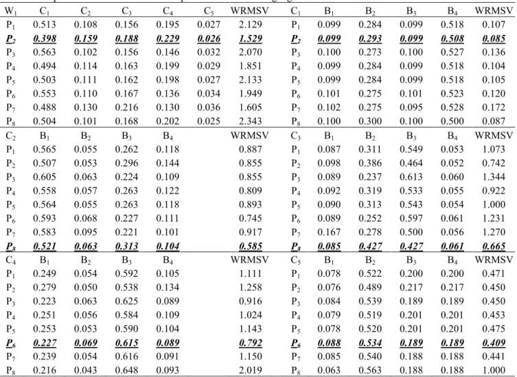
P p p {EV, NRS, NRCS, AMNC, NGNR/LLS, WLS, FP, GP}. Table 1 shows the priorities and WRMSV for six pairwise matrices using eight prioritization operators. The best prioritization operator is the one with the least WRMSV. The result of using the method proposed by Kulak and Kahramna [9] is the same as the result obtained when using P4 (AMNC). The Saaty’s Eigen vector method is P1. It can be
observed that neither of these two, in the six matrices is selected as the best PO. The best PO is the one with the fonts of bold, italic and underlined in Table 1. In the six matrices, the best POs are P2, P2, P8, P8, P6, and P6. It can be concluded that the best PO is case dependant as no PO can outperform other POs in all matrix cases.
Table 1: The priorities and WRMSV for six pairwise matrices using eight POs
W1 C1 C2 C3 C4 C5 WRMSV C1 B1 B2 B3 B4 WRMSV
P1 0.513 0.108 0.156 0.195 0.027 2.129 P1 0.099 0.284 0.099 0.518 0.107
P2 0.398 0.159 0.188 0.229 0.026 1.529 P2 0.099 0.293 0.099 0.508 0.085
P3 0.563 0.102 0.156 0.146 0.032 2.070 P3 0.100 0.273 0.100 0.527 0.136
P4 0.494 0.114 0.163 0.199 0.029 1.851 P4 0.099 0.284 0.099 0.518 0.104
P5 0.503 0.111 0.162 0.198 0.027 2.133 P5 0.099 0.284 0.099 0.518 0.105
P6 0.553 0.110 0.167 0.136 0.034 1.949 P6 0.101 0.275 0.101 0.523 0.120
P7 0.488 0.130 0.216 0.130 0.036 1.605 P7 0.102 0.275 0.095 0.528 0.172
P8 0.504 0.101 0.168 0.202 0.025 2.343 P8 0.100 0.300 0.100 0.500 0.087
C2 B1 B2 B3 B4 WRMSV C3 B1 B2 B3 B4 WRMSV
P1 0.565 0.055 0.262 0.118 0.887 P1 0.087 0.311 0.549 0.053 1.073
P2 0.507 0.053 0.296 0.144 0.855 P2 0.098 0.386 0.464 0.052 0.742
P3 0.605 0.063 0.224 0.109 0.855 P3 0.089 0.237 0.613 0.060 1.344
P4 0.558 0.057 0.263 0.122 0.809 P4 0.092 0.319 0.533 0.055 0.922
P5 0.564 0.055 0.263 0.118 0.893 P5 0.090 0.313 0.543 0.054 1.000
P6 0.593 0.068 0.227 0.111 0.745 P6 0.089 0.252 0.597 0.061 1.231
P7 0.583 0.095 0.221 0.101 0.917 P7 0.167 0.278 0.500 0.056 1.270
P8 0.521 0.063 0.313 0.104 0.585 P8 0.085 0.427 0.427 0.061 0.665
C4 B1 B2 B3 B4 WRMSV C5 B1 B2 B3 B4 WRMSV
P1 0.249 0.054 0.592 0.105 1.111 P1 0.078 0.522 0.200 0.200 0.471
P2 0.279 0.050 0.538 0.134 1.258 P2 0.076 0.489 0.217 0.217 0.450
P3 0.223 0.063 0.625 0.089 0.916 P3 0.084 0.539 0.189 0.189 0.450
P4 0.251 0.056 0.584 0.109 1.024 P4 0.079 0.519 0.201 0.201 0.453
P5 0.253 0.053 0.590 0.104 1.143 P5 0.078 0.520 0.201 0.201 0.475
P6 0.227 0.069 0.615 0.089 0.792 P6 0.088 0.534 0.189 0.189 0.409
P7 0.239 0.054 0.616 0.091 1.150 P7 0.085 0.540 0.188 0.188 0.441
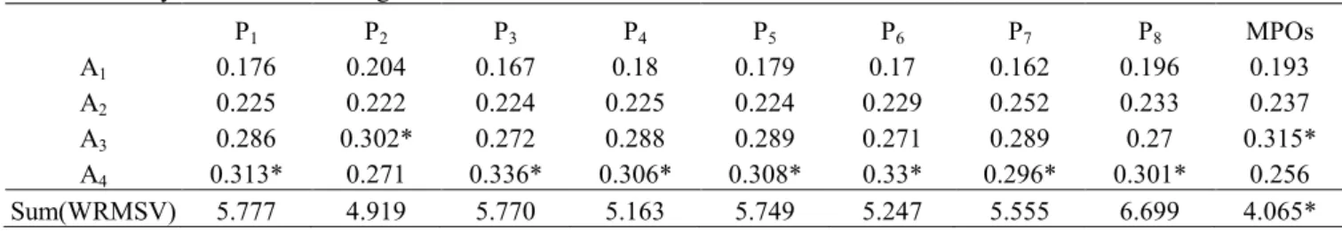
Table 2: The synthesis results of eight POs and a Mixed POs method
P1 P2 P3 P4 P5 P6 P7 P8 MPOs
A1 0.176 0.204 0.167 0.18 0.179 0.17 0.162 0.196 0.193
A2 0.225 0.222 0.224 0.225 0.224 0.229 0.252 0.233 0.237
A3 0.286 0.302* 0.272 0.288 0.289 0.271 0.289 0.27 0.315*
A4 0.313* 0.271 0.336* 0.306* 0.308* 0.33* 0.296* 0.301* 0.256
Sum(WRMSV) 5.777 4.919 5.770 5.163 5.749 5.247 5.555 6.699 4.065*
Table 2 shows the results of a synthesis of eight POs and a Mixed POs (MPOs) method. p1,,p8 apply a pure PO strategy to derive the local priorities, and then synthesize the result. The result shows that p p1, 3,,p8 support the fact that the transportation company 4 is the best candidate whilst p2 and the MPOs method show that company 3 is the best. To measure the results, the WRMSVs of all pairwise matrices for all methods are summed up. It can be found that P2 and MPOs are with the least two summation
of WRMSVs. In this example, summation of WRMSV, more than five possible produce inaccurate results. Although NRS (P2) is the most straightforward, its
accuracy probably is better than other methods. This result is supported by MPOs. As MPOs apply the best PO regarding cases, the result of MPOs are much better than the pure PO method.
The results of many of the transportation studies in AHP stated in the introduction section are dubious as the studies only applied a pure PO strategy using the Eigenvalue method without comparison with other prioritization operators. The Mixed POs strategy is recommended, especially for those quantitative and qualitative researches with subjective measurement weights. The literature reviews also find most of the studies did not incorporate the data of the pairwise matrix to derive the weights which are further propagated with other criteria measurement data. Thus some research findings are questionable.
V. CONCLUSION
The most appropriate prioritization method is still one of the unsettled issues of Analytic Hierarchy Process theory, although many studies have been done and applied. Interestingly, many studies of transportation evaluation and selection models using AHP use only a single prioritization method: Saaty’s Eigenvector method. Many theoretical studies have found this method to be unsatisfactory and have proposed various prioritization methods as alternatives. Some have proved to be superior to the
Eigenvector method. However, a literature review shows that these methods seem not to attract the attention of researchers in this research area.
In this paper, a Mix Prioritization Operators strategy is proposed to address this issue. Eight important prioritization operators are reviewed: Eigenvector method, Normalization of the Row Sum, Normalization of Reciprocals of Column Sum, Arithmetic Mean of Normalized Columns, Row Geometric Mean or Logarithm Least Squares, Weighted Least Squares, Fuzzy Programming, and Goal Programming. The Weighted Root Mean Square Variance method, which combines the advantages and offsets the disadvantages of Root Mean Square Variance and Mean Minimum Violation, is proposed for the selection of the best PO for solving AHP Transportation problems.
To ensure the validity and usability of this new model, one case study selected from Kulak and Kahramna [9] is used to compare the outcomes of the Pure PO strategy and the Mixed POs strategy. The research result shows that a single pure PO strategy possibly produces unreliable results as it may have high Weighted Root Mean Square Variance. On the other hand, the MPOs strategy can produce more convincing results than the pure PO strategy since the multiple best prioritization operators are used to minimize the approximate variance. The contribution of this paper is that the MPOs model may be used as the guidelines for developing an AHP transportation model, especially for the important unsettled issue regarding the prioritization problem in AHP.
APPENDIX
The following two tables are the summary of the details of the transportation company selection problem using crisp AHP, which is adopted from Kulak and Kahramna [9].
Table A1: Criteria and alternatives
Criteria Description Labels Alternatives Labels
TC Transportation Cost C1 Transport Company 1 B1
DR Defective rate C2 Transport Company 2 B2
TR Tardiness Rate C3 Transport Company 3 B3
F Flexibility C4 Transport Company 4 B4
Table A2: The Pairwise matrices
C TC DR TR F DA C1 B1 B2 B3 B4
TC 1.00 5.00 3.00 5.00 9.00 B1 1.00 0.33 1.00 0.20
DR 0.20 1.00 0.50 0.50 7.00 B2 3.00 1.00 3.00 0.50
TR 0.33 2.00 1.00 0.50 7.00 B3 1.00 0.33 1.00 0.20
F 0.20 2.00 2.00 1.00 8.00 B4 5.00 2.00 5.00 1.00
DA 0.11 0.14 0.14 0.13 1.00
C2 B1 B2 B3 B4 C3 B1 B2 B3 B4
B1 1.00 7.00 3.00 5.00 B1 1.00 0.20 0.20 2.00
B2 0.14 1.00 0.20 0.33 B2 5.00 1.00 0.33 7.00
B3 0.33 5.00 1.00 3.00 B3 5.00 3.00 1.00 7.00
B4 0.20 3.00 0.33 1.00 B4 0.50 0.14 0.14 1.00
C4 B1 B2 B3 B4 C5 B1 B2 B3 B4
B1 1.00 5.00 0.33 3.00 B1 1.00 0.20 0.33 0.33
B2 0.20 1.00 0.14 0.33 B2 5.00 1.00 3.00 3.00
B3 3.00 7.00 1.00 7.00 B3 3.00 0.33 1.00 1.00
B4 0.33 3.00 0.14 1.00 B4 3.00 0.33 1.00 1.00
ACKNOWLEDGMENTS
The author also wishes to thank the Research Office of the Hong Kong Polytechnic University for support of this research project. Thanks in advance are also extended to the editors and anonymous referees for their constructive criticisms to improve this research work.
REFERENCES
[1] J. Aguaron, J. M. Moreno-Jimenez, The geometric consistency index: Approximated thresholds. European Journal of Operational Research 147 (2003) 137–145.
[2] N. Bryson, A goal programming method for generating priorities vectors. J Opl Res Soc 46 (1995) 641-648.
[3] H. Cercek, B. Karpak, T. Kilincaslan, T. A multiple criteria approach for the evaluation of the rain transit networks in Istanbul. Transportation 31 (2004) 203-228.
[4] E.U. Choo, W.C. Wedley, A common framework for deriving preference values from pairwise comparison matrices, Computer & Operations Research 31 (2004) 893-908.
[5] A.T.W. Chu, R.E. Kalaba, K. Springarn, A comparison of two methods for determining the weights of belonging to fuzzy sets. J Opt Theory and Appl. 27 (1979) 531-541.
[6] G. Crawford, C. Williams, C. A note on the analysis of subjective judgement matrices. J. Math Psychol 29 (1985) 387-405. [7] P. Ferrari, A method for choosing from among alternative
transportation projects, European Journal of Operation Research 150 (2003) 194-203
[8] B. Golany, M. Kress, A multicriteria evaluation of methods for obtaining weights from ratio-scale matrices, Eur J Opl Res 69 (1993) 210-220.
[9] O. Kulak, C. Kahraman, Fuzzy multi-attribute selection among transportation companies using axiomatic design and analytic hierarchy process. Information Sciences 170 (2005) 191-210. [10] L. Mikehailov, M.G. Sing, comparison analysis of methods for
deriving priorities in the analytic hierarchy process. Proceedings of the IEEE International conference on Systems, Man and Cybernetics, 1999, 1037-1042.
[11] L. Mikehailov, A Fuzzy Programming Method for Deriving Priorities in the Analytic Hierarchy. The Journal of the Operational Research Society 51(3) (2000) 341-349.
[12] T.L. Saaty, Scenarios and priorities in transport planning: Application to Sudan. Transportation Research 11A (1977) 343-350
[13] T.L. Saaty, Analytic Hierarchy Process: Planning, Priority, Setting, Resource Allocation: McGraw-Hill: New York, 1980
[14] T.L. Saaty, L.G. Vargas, Comparison of Eigenvalue, Logarithmic Least Squares and Lest Squares Methods In Estimating Ratios, Mathematical Modelling 5 (1984) 309-324
[15] T.L. Saaty, Transport planning with multiple criteria: the analytic Hierarchy Process Applications and Progress Review, Journal of Advanced Transportation, 29 (1) (1995) pp.81-126
[16] K Sohn, A systematic decision criterion for the elimination of useless overpasses. Transportation Research Part A, 2008, Online. [17] B. Srdjevic, Combining different prioritization methods in the analytic hierarchy process synthesis. Computers and Operations Research 32 (2005) 1897-1919.
[18] P. Tanadtang, D. Park, S. Hanaoka, Incorporating uncertain and incomplete subjective judgment into the evaluation procedures of transportation demand management alternatives. Transportation 32(6) (2005) 603-626.
[19] K.K.F. Yuen, A Compound Linguistic Ordinal Scales Model: A Breakthrough of the Magical Number Seven, Plus or Minus Two. Information Sciences, 2009, under revision.
[20] K.K.F Yuen, Analytic Hierarchy Prioritization Process in the AHP Applications Development: A Prioritization Operator Selection Approach, 2009, working paper.
[21]K.K.F Yuen, Measuring Software Quality using a Fuzzy Group Analytical Hierarchy Process Model with ISO/IEC 9126, 2009, working paper.
[22] K.K.F. Yuen, H.C.W. Lau, Evaluating Software Quality of Vendors using Fuzzy Analytic Hierarchy Process, Lecture Notes in Engineering and Computer Science, IMECS 2008, Volume I, pp126-130