COMBINATIONS OF ADAPTIVE FILTERS
COMBINATIONS OF ADAPTIVE FILTERS
Disserta¸c˜ao apresentada `a Escola Polit´ecnica da Universidade de S˜ao Paulo para obten¸c˜ao do T´ıtulo de Mestre em Ciˆencias.
COMBINATIONS OF ADAPTIVE FILTERS
Disserta¸c˜ao apresentada `a Escola Polit´ecnica da Universidade de S˜ao Paulo para obten¸c˜ao do T´ıtulo de Mestre em Ciˆencias.
´
Area de Concentra¸c˜ao:
Sistemas Eletrˆonicos
Orientador:
Prof. Dr. C´assio G. Lopes
I would like to thank my advisor, Prof. C´assio G. Lopes, for his guidance and indelible advice, as well as for the constant challenges and opportunities that kept me motivated.
I would also like to thank my parents, Marco and Edna, for all their support over these years, and my brother Paulo for the conversations and debates that keep me on my toes.
It is difficult to express my gratitude to my friends at the University of S˜ao Paulo, Wilder, Fernando, Amanda, Renato, David, Matheus, Yannick, and Humberto, for their help in both shaping this work and, at times, forgetting about it.
I am also indebted to all my professors, at the University of S˜ao Paulo and elsewhere, for having shared their knowledge, opinions, and experience. In particular, I would like to thank Prof. V´ıtor Nascimento and Prof. Magno Silva for their contributions to this work and to my formation.
Finally, I cannot thank enough my beloved fianc´ee B´arbara B. Lucena for her presence, support, and understanding in good and bad times.
1 The analogy: (a) schema of a member and (b) the workgroup . . . 15
2 The system identification scenario . . . 22
3 A supervised adaptive filter . . . 24
4 Physical interpretation of the ECR: (a) general adaptive filter; (b) NLMS (to-tal reflexion) . . . 27
5 Combination of adaptive filters . . . 30
6 FOB description . . . 30
7 A digraph D= (V, A) . . . 32
8 Example digraphs of combination topologies: (a) stand-alone adaptive fil-ter; (b) arbitrary topology. . . 33
9 Data distribution networks: (a) data sharing; (b) stand-alone data reusing adaptive filter; (c) circular buffer; (d) randomized. . . 38
10 FOB description of adaptive networks: (a) incremental and (b) diffusion. . 45
11 Timeline . . . 49
12 Taxonomy of combinations of adaptive filters . . . 51
13 Hierarchical parallel combination of four adaptive filters . . . 58
14 The parallel-independent topology digraph. . . 62
15 Convergence stagnation issue of the parallel-independent topology . . . 63
16 The parallel topology with coefficients leakage digraph. . . 64
17 The parallel topology with cyclic coefficients feedback digraph. . . 64
18 Comparison between coefficients leakage and coefficients feedback . . . 65
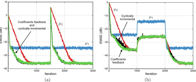
19 Tracking of an LMS+RLS combination with and without coefficients feedback 67 20 2·LMS combination with coefficients feedback (L= 1) . . . 68
23 The effect of the convexity constraint on the incremental supervisor . . . . 74
24 Comparison between different supervising rules for a combination of two LMS filters. . . 75
25 Incremental topology digraphs: (a) linear incremental topology and (b) ring incremental topology. . . 75
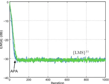
26 Comparison between the {LMS}N and the APA. . . 77
27 Cyclically incremental, parallel combination of LMS filters . . . 79
28 Graph representation of parallel-incremental topologies: (a) parallel com-bination of incremental components and (b) parallel comcom-bination of incre-mental combinations. . . 80
29 Parallel-incremental combination of LMS filters . . . 81
30 Variable step size algorithm based on a 2·LMS combination with coefficients feedback (nonstationary SNR) . . . 85
31 Variable step size algorithm based on a 2·LMS combination with coefficients feedback (nonstationary wo ) . . . 86
32 Graphical representation of the complexity of different algorithms with similar performances . . . 88
33 Diagram of relations between the APA and combinations of adaptive filters 88 34 APA and f{K·LMS} . . . 91
35 APA and DR-{LMS}N (stationary scenario) . . . 92
36 APA and DR-{LMS}N (nonstationary scenario) . . . 93
37 Parallel-incremental combination (white input) . . . 94
38 Parallel-incremental combination (correlated input) . . . 95
39 Performance of the {sign-error LMS}N in fixed point precision (stationary scenario) . . . 96
40 Performance of the{sign-error LMS}N in fixed point precision (nonstation-ary scenario) . . . 97
43 Steady-state of parallel combinations with cyclic coefficients feedback for
different cycle periods . . . 105
44 Steady-state analysis of a 2·LMS combination . . . 113
45 Tracking analysis of a 2·LMS combination . . . 113
46 Steady-state analysis of an LMS + LMF combination . . . 115
47 Tracking analysis of the LMMN using an LMS + LMF combination. . . 116
48 Steady-state analysis of a 2·RLS combination . . . 119
49 Tracking analysis of an LMS + RLS combination . . . 121
50 Supervising parameter variance under different topologies (normalized con-vex supervisor . . . 128
51 Transient analysis of a 2·LMS combination with a convex supervisor. . . . 129
52 Transient analysis of the 2·LMS combination with an affine supervisor . . 130
53 Separation principle A.13 . . . 136
54 Steady-state analysis validation . . . 138
55 Mean convergence analysis of an {LMS}N . . . 140
56 Incremental mean-square analysis of a {LMS}2 . . . 144
1 Motivation, contributions, and notation 14
1.1 An analogy: The workgroup . . . 14
1.2 Motivation . . . 15
1.3 Objectives . . . 16
1.4 Contributions . . . 17
1.5 Publications list . . . 17
1.6 Notation . . . 18
1.6.1 The system identification scenario . . . 20
2 Stand-alone adaptive filters 23 2.1 Figures of merit . . . 25
2.2 Energy conservation relation . . . 26
2.3 Concluding remarks . . . 28
3 Combinations of adaptive filters 29 3.1 A formal definition . . . 29
3.2 The topology . . . 31
3.2.1 Digraphs . . . 31
3.2.2 Topologies and digraphs . . . 32
3.2.3 The parallel/incremental dichotomy . . . 34
3.3 The data reusing method . . . 36
3.3.1 Data distribution networks . . . 38
3.4 The supervisor . . . 40
3.7 Concluding remarks . . . 46
4 Taxonomy and review 47 4.1 Timeline . . . 47
4.2 Classifying combinations . . . 50
4.2.1 Component filters . . . 52
4.2.2 Topology . . . 52
4.2.3 Data reusing method . . . 52
4.2.4 Supervising rule . . . 52
4.3 Concluding remarks . . . 53
5 Parallel combinations 56 5.1 Supervising rules . . . 56
5.1.1 Unsupervised (“static”) . . . 58
5.1.2 The convex supervisor . . . 59
5.1.3 The affine supervisor . . . 60
5.2 Parallel topologies . . . 61
5.2.1 The parallel-independent topology . . . 61
5.2.2 The parallel topology with coefficients leakage . . . 63
5.2.3 The parallel topology with coefficients feedback . . . 65
5.2.3.1 Design of the cycle period . . . 66
5.3 Concluding remarks . . . 68
6 Incremental combinations 71 6.1 Supervising rules . . . 72
6.1.1 Unsupervised (“static”) . . . 73
6.2 Incremental topologies . . . 74
6.2.1 Linear incremental topology . . . 75
6.2.2 Ring incremental topology . . . 76
6.3 Concluding remarks . . . 76
7 Combinations with arbitrary topologies 78 7.1 Cyclically incremental, parallel topology . . . 78
7.2 Parallel-incremental combination . . . 79
7.3 Concluding remarks . . . 80
8 Stand-alone adaptive algorithms as combinations of adaptive filters 82 8.1 Mixed cost function algorithms . . . 82
8.2 Data reusing algorithms . . . 83
8.3 Variable step size algorithms . . . 84
8.4 Concluding remarks . . . 85
9 Combination as a complexity-reduction technique 87 9.1 DR-{LMS}N . . . 88
9.1.1 The APA and the f{K·LMS} . . . 88
9.1.2 The incremental counterpart of f{K ·LMS} . . . 90
9.2 DR-{LMS}N + LMS . . . 92
9.3 {sign-error LMS}N . . . 93
9.4 DR-{sign-error LMS}N L . . . 97
9.5 Concluding remarks . . . 97
10 Performance analysis of parallel combinations 101 10.1 Steady-state and tracking performance . . . 101
10.1.3 Variance and covariance relations for L→ ∞. . . 105
10.1.4 Variance and covariance relations for L= 1 . . . 107
10.1.5 Supervisor analysis . . . 109
10.2 Steady-state and tracking performance of specific combinations . . . 111
10.2.1 2·LMS . . . 111
10.2.1.1 Without feedback . . . 111
10.2.1.2 With feedback . . . 112
10.2.2 LMS + LMF . . . 113
10.2.2.1 Without feedback . . . 114
10.2.2.2 With feedback . . . 115
10.2.3 2·RLS . . . 116
10.2.3.1 Without feedback . . . 117
10.2.3.2 With feedback . . . 118
10.2.4 LMS + RLS . . . 119
10.2.4.1 Without feedback . . . 119
10.2.4.2 With feedback . . . 120
10.3 Transient Performance . . . 121
10.3.1 Component filters analysis . . . 122
10.3.2 Supervisor analysis . . . 125
10.3.3 Complete transient analysis . . . 127
10.4 Concluding remarks . . . 128
11 Performance analysis of incremental combinations 132 11.1 Overall recursion . . . 133
11.2 Steady-state performance . . . 134
11.3 Transient performance . . . 139
11.3.1 Mean convergence analysis . . . 139
11.3.2 Unbiasedness constraint . . . 141
11.3.3 Mean-square convergence analysis . . . 142
11.3.4 Optimal supervisor . . . 144
11.4 Concluding remarks . . . 146
12 Conclusion 148
13 Suggestions for future work 149
1
MOTIVATION, CONTRIBUTIONS, AND
NOTATION
Analogies prove nothing, that is quite true, but they can make one feel more at home.
-- Sigmund Freud, “New Introductory Lectures on Psychoanalysis”
1.1
An analogy: The workgroup
Analogies used in the context of local or distributed adaptive signal processing usually involve some sort of learning experience [1–6]. These, however, are limited inasmuch as they only deal with the adaptation capability of the algorithms without explicitly addressing the estimation/filtering step. What is more, distributed scenarios require
an analogy for the exchange of information between nodes and the direct passing of “learned concepts” among peers is hard to relate to our own experience with knowledge transmission. An extension of the typical analogy is therefore proposed below.
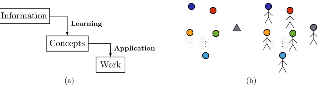
Define a workgroup as a set of peers that collaborate to achieve a common goal. Each member relies on the information available to him to learn concepts and apply these concepts to produce work (Figure 1a). The latter step is the fundamental difference with previous analogies, as the members of the workgroup no longer only learn but also perform an action based on their learning. The workgroup has a leader (supervisor) responsible for generating a single piece of work based on the work produced by the group members1.
In a more concrete example, the information available can be thought of as books and the goal is to write an essay (e.g., a dissertation on combinations of adaptive filters). The assignment of the group leader is then to hand in a unique essay based on those written by the members, as well as the available books.
Individually, the group members may have different reading/learning/writing charac-teristics. Some may be more careful and take longer to deliver their version of the essay,
while others work faster at the cost of making more mistakes. Also, the books available to the workgroup share a common topic and may therefore repeat themselves (their in-formation is correlated). Some members may be better than others at identifying and
1
(a) (b)
Figure 1: The analogy: (a) schema of a member and (b) the workgroup
skipping these parts. Finally, it could be that the concept under study is still under debate (nonstationary) and people’s ability to update their essays to reflect changes can vary. The objective of working in a group is taking advantage of each member’s strength while counterbalancing their weaknesses.
But how to organize this cooperation? Should the members write their essays
inde-pendently (parallel-independent topology, Chapter 5) or should they take turns writing the final essay (incremental topology, Chapter 6)? Should the group leader give feedback on the members work (coefficients feedback, Section 5.2.3)? Is it better for all workers to read the same book or should they each get a different one (data reusing method,
Section 3.3)? The same questions can be asked for combinations and the result of their analyses in the remainder of this work can be interpreted in the context of the workgroup analogy.
1.2
Motivation
As is usually the case in engineering, estimation and detection problems come with
trade-offs and limitations that may be hard to overcome (e.g., bias/variance or type I/type II errors compromises [8,9]). Combination is an established pattern to address this situation in several domains.
In the context of universal prediction, for example, algorithms with different predictive capabilities are weighted and aggregated to form a more robust predictor [10–12]. In fact, such an algorithm selection approach can be used to construct a “deterministic”
weak and strong learnability are actually equivalent. These algorithms are among the most effective ones in ML today [17].
Adaptive filters (AFs) are well-suited for combinations due to the compromises in-volved in their applications. Indeed, despite their versatility, AFs have inherent trade-offs
that usually hinge on three aspects: transient performance, steady-state performance, and computational complexity. For instance, increasing the convergence rate of an adap-tive algorithm typically involves degrading its steady-state error level [18–20]. Otherwise, another more complex AF must be used (such as the APA or RLS). Many of these
algo-rithms, however, suffer from robustness issues that hinder their use in some scenarios (e.g., highly correlated signals and reduced precision [18, 19, 21]). Other solutions have been proposed, such as data reusing (DR) [22–25], mixed-norm updates [26–29], and variable step size (VSS) [30–32]. Combinations of AFs, however, have shown several advantages over these techniques in terms of performance and robustness [33–49]. In some cases, it even provides a more general framework under which these adaptive algorithms can be cast (as argued in Chapter 8).
1.3
Objectives
This work proposes to study combinations of AFs in a general and unified way. In doing so, it bridges the gap between different combinations, as well as combinations and
stand-alone AFs, that were previously not properly related. The objectives of this research can be stated as:
I. Classify existing combinations
The development of a taxonomy for combinations of AFs helps clarify the similarities
between existing combinations and better understand the elements that constitute these structures. This classification and the similarities found constitute an impor-tant step towards Objectives II and III.
II. Propose new combinations
Based on the classification devised for Objective I, unexplored algorithms/combinations
can be investigated to formulate new structures that can then be analyzed and com-pared to the existing ones. These analyses can then be used to improve the general framework of Objective III.
III. Devise a general framework for combinations of adaptive filters
framework for combinations can be created. This framework involves the formulation of a precise definition of combination of AFs, through which performance analyses
can be derived. These analyses contribute to a better understanding of combinations and, thus, to Objective I.
1.4
Contributions
(i) Extensive literature review and a taxonomy to classify combination of adaptive filters.
(ii) A definition of combination and combination of adaptive filters, along with a specific notation to describe them.
(iii) A formal study of combination topology using graph-theoretic arguments.
(iv) Parallel topology with cyclic coefficients feedback: motivation, proposition, and
anal-yses.
(v) Data reusing combinations: motivation, data distribution networks, and perfor-mance improvements.
(vi) Interpreting stand-alone adaptive algorithms as combinations of AFs and bridging the gap between combinations and adaptive networks.
(vii) Combination as a complexity reduction technique.
(viii) Unified performance analysis of parallel combinations: energy conservation relation, steady-state, tracking, and transient behavior for different component filters and
supervising rules.
(ix) Performance analysis of incremental combinations: steady-state, transient, unbi-asedness constraint, and optimal supervisor.
1.5
Publications list
[1] L.F.O. Chamon and C.G. Lopes. “Combinations of adaptive filters with coefficient feedback”. Work in progress (Journal), 2015.
[3] L.F.O. Chamon and C.G. Lopes. “There’s plenty of room at the bottom: Incremental combinations of sign-error LMS filters”. In: International Conference in Acoustic, Speech, and Signal Processing (ICASSP), p. 7248–7252, 2014.
[4] L.F.O. Chamon and C.G. Lopes. “Transient performance of an incremental combina-tion of LMS filters”. In: European Signal Processing Conference (EUSIPCO), 2013. [5] L.F.O. Chamon and C.G. Lopes. “On parallel-incremental combinations of LMS filters
that outperform the Affine Projection Algorithm”. In: Brazilian Telecommunication Symposium (SBrT), 2013.
[6] L.F.O. Chamon, H.F. Ferro, and C.G. Lopes. “A data reusage algorithm based on in-cremental combination of LMS filters”. In: Asilomar Conference on Signals, Systems and Computers, p. 406–410, 2012.
[7] L.F.O. Chamon, W.B. Lopes, and C.G. Lopes. “Combination of adaptive filters with coefficients feedback”. In: International Conference in Acoustic, Speech, and Signal Processing (ICASSP), p. 3785–3788, 2012.
[8] L.F.O. Chamon and C.G. Lopes. “Combination of adaptive filters for relative
naviga-tion”. In: European Signal Processing Conference (EUSIPCO), p. 1771–1775, 2011.
1.6
Notation
The main conventions and symbols used in this work are collected in Table 1. In particular, note thatboldfaceis used to denote vectors and matrices and that all vectors are column vectors except for the regressor vector u, which is taken as a row vector for convenience. When iteration-dependent, scalars are indexed as in x(i) and vectors as
inxi. All variables in this text are real-valued2. Deterministic and random variables are
clear from the context.
In the context of combinations, component filters values are indexed by n. For in-stance,en(i),wn,i, and{un,i, dn(i)} refer to the n-th component output estimation error,
coefficient vector, and data pair, all at iteration i. Buffered data, on the other hand,
are indexed using k. Thus, the k-th data pair in the buffer (k-th row of Ui and di) is
referred to as{uk,i, dk(i)}. Often times,{uk,i, dk(i)}={ui−k, d(i−k)}, in which case the
2
latter form is preferred for explicitness. Notice that component filters and input data use different indices (n and k, respectively), a distinction that is important when discussing
DR methods. Also relative to combinations, variables without the n index refers to a global quantity (e.g., the global coefficientswi or the output of the combination y(i)).
When referring to combinations, the notation introduced in [45, 47] is adopted in this text to avoid the use of long cryptic acronyms. Inspired by transfer function composition in system theory [51], parallel combinations are represented byaddition, whereas incremental combinations are represented by multiplication. Typical precedence rules and intuitive extensions can be used as shorthands for larger combinations. For instance, for two LMS filters, their parallel combination is written LMS + LMS or 2·LMS and their incremental combination, LMS· LMS or {LMS}2. When necessary, combinations with coefficients
feedback ordata buffering are distinguished using the prefixesf or DR respectively, as in
f{LMS + LMS} and DR-{LMS}N.
In the sequel, the data model and assumptions used in the performance analyses and simulations are introduced.
Table 1: List of symbols and notation
R Field of real numbers
Z Ring of integer numbers
N Set of natural numbers
I Identity matrix
1 Column vector of ones
(·)T Matrix transposition
diag{x} Diagonal matrix formed from the entries of x
kxk Euclidian norm of x
kxkW Weighted norm of x(xTW x)
kxk1 ℓ1-norm of x
|x| Absolute value of the scalar x. Applies element-wise to a vector
δ(i) Kronecker delta
δL(i) Impulse train of period L: δL(i) = Pr∈Nδ(i−rL)
u(i) Input signal
ui Regressor vector (1×M)
Ru Covariance matrix of the regressor vector u
σ2
u Variance of the input signal u(i)
v(i) Noise
σ2
v Variance of the noise v(i)
wo
Unknown system coefficient vector (M ×1) qi System disturbance vector (M ×1)
Q System disturbance covariance matrix
d(i) Scalar measurement
Ui Buffer of regressor vectors (K×M matrix)
di Buffer of measurements (K ×1 vector)
wi Overall (global) coefficient vector y(i) Output of the combination
e(i) Overall (global) output estimation error
ea(i) Overall (global)a priori error
ep(i) Overall (global) a posteriori error e
wi Overall (global) coefficients error vector ηn(i) Supervising parameter for then-th component filter {un,i, dn(i)} Data pair (input) of the n-th component filter
wn,i Coefficient vector of then-th component filter
wn,a A priori coefficient vector of the n-th component filter yn(i) Output of the n-th component filter
en(i) Output estimation error of then-th component filter
ea,n(i) A priori error of the n-th component filter
ep,n(i) A posteriori error of the n-th component filter e
wn,i coefficients error vector of the n-th component filter µn n-th component filter step size
1.6.1
The system identification scenario
AFs can be used in a myriad of scenarios and setups, such as equalization, inverse control, and prediction [18–20]. However, for the purpose of performance analysis and simulation, a system identification scenario (Figure 2) is usually adopted [18–20], as it is representative of many applications, such as echo cancellation [52, 53], time delay
estima-tion [54–59], and adaptive control [60].
measure-ments
d(i) = uiw
o
i +v(i), (1.1)
wherewo
i is anM×1 vector that represents the unknown system at iterationi, ui is the
1×M regressor vector (with covariance matrixRu= EuTi ui) that captures samplesu(i)
of a zero mean input signal with varianceσ2
u, andv(i) is a zero mean i.i.d. sequence with
varianceσ2
v that represents the measurement noise. The samples{u(i), v(i)} are assumed
to be realization of a Gaussian real-valued random process and to follow A.1 below. This
assumption is used to render the derivations more tractable, since in practice the noise is at most uncorrelated with the input [18].
A.1 (Noise independence){v(i),uj} are independent for all i, j.
To account for different types of input in simulations, a Gaussian i.i.d. RV x(i) is used to generate the samplesu(i). For white input data, u(i) =x(i). On the other hand, to simulate input data correlation, a first-order AR model [AR(1)] is adopted [18, 19]. Explicitly,
u(i) =γ u(i−1) +p1−γ2x(i), (1.2)
for some parameter 0 < γ < 1 that control the degree of correlation (the closer to one, the more correlated).
To model nonstationary systems, the following first order random walk is adopted [18, 19]:
wio =wio−1+qi, (1.3)
where the initial state iswo
−1 =w
o
andqi is the realization of a zero mean i.i.d. Gaussian
RV with covariance matrixQ= EqiqTi . When the system is stationary, qi =0⇒Q=0
and wo
i =w
o
. For tractability of the analysis, assume that
A.2 (Random walk independence assumption) The RV qi is statistically independent of
the initial conditions {wo
−1,w−1}, of {uj, v(j)}for all i, j, and of {d(j)}for i > j.
When studying DR techniques, it is convenient to define the data buffersUi = [ ui−k ],
aK×M regressor matrix, and di = [ d(i−k) ], aK×1 measurement vector, fork ∈ K,
whereK ⊂Z+ is an index set of size K. A typical choice would be [18, 19, 61]
Ui =
ui
ui−D
... ui−(K−1)D
and di =
d(i)
d(i−D) ...
-+
Figure 2: The system identification scenario
The delayD between regressors was introduced in [62] to reduce the correlation between
rows in Ui, which decreases the condition number of UiUiT whose inverse is used in the
recursion of some adaptive algorithms [18, 19]. Notice that the data model (1.1) can be written in terms of the buffers in (1.4) as
di =Uiw
o
+vi, (1.5)
where vi = [ v(i) v(i−D) · · · v[i−(K −1)D] ]T. Observe that for K = 1, (1.5)
2
STAND-ALONE ADAPTIVE FILTERS
O todo sem a parte n˜ao ´e todo, A parte sem o todo n˜ao ´e parte, Mas se a parte o faz todo, sendo parte, N˜ao se diga, que ´e parte, sendo todo.1
-- Greg´orio de Matos, “Ao bra¸co do mesmo Menino Jesus quando apareceu”
Adaptive filtering originated with the introduction of the Least Mean Squares (LMS) filter in the beginning of the 1960s by Widrow and Hoff [1]. Since then, it has gained considerable attention from the signal processing community and the number of adaptive algorithms and their applications have grown quickly (see [18–20,52,60,63] and references
therein).
An AF can be defined as a pairfiltering structure–adaptation algorithm (Figure 3) [20]. It is important to distinguish this configuration from the statistics estimator–Wiener solver pair, which estimates statistical properties from the data and plugs them into a non-recursive formula for computing the filter parameters (which Haykin [20] calls the
estimate-and-plug procedure). This second approach does not take advantage of iterative solutions, which are able to provide partial results as they converge. Furthermore, it most certainly leads to more complex algorithms. Considering this definition, the present work studies the class of AFs that employs Finite Impulse Response (FIR) filters adapted
by means of supervised algorithms [18–20]. Note, however, that there is no restriction as to the algorithms that can be combined and combinations involving Infinite Impulse Response (IIR) [48, 64] and unsupervised [34, 65, 66] AFs are also possible.
Explicitly, a supervised adaptive algorithm is a procedure to update, at iteration i, ana priori coefficient vector wa using a data pair {ui, d(i)} (or more generally, {Ui,di})
so as to minimize a scalar cost functionJ(wa). Most often, this is done using a stochastic
gradient method [18–20] of general form
wi =wa−µp, (2.1)
where µ is a step size, p = B∇TJ(w
a) is an update direction, and B is a symmetric
1
-+
Figure 3: A supervised adaptive filter
positive-definite matrix.
The introduction of the concept of a priori coefficients in (2.1) is motivated by the view of AFs as solvers of local optimization problems [18]. From this viewpoint, an AF is a general algorithm that updates any givenwa according to its cost function. Even though
most of them are made recursive by choosingwa =wi−1, the advantage of adopting (2.1)
is that it accounts for interruptions in the regular operation of the adaptive algorithm, such as reinitializations or rescue techniques [18]. Moreover, the a priori coefficient vector is fundamental in the derivation of a general definition of combinations of AFs in Chapter 3. For the sake of clarity, however, the remainder of this chapter assumes wa =wi−1.
Different choices of p lead to different adaptive algorithms [18]. In stand-alone adaptive filtering, the cost function is typically chosen as the mean-square error (MSE)
J(wi−1) = Ee2(i), where e(i) = d(i)−y(i) is the output estimation error and y(i) =
uiwi−1 is the output of the AF [18–20]. Nevertheles, other functions have also been
successfully used. The recursion of the AFs found in this work are collected below for reference1:
wi =wi−1+µuTi e(i) (LMS [1, 18]) (2.2)
wi =wi−1+µuTi sign[e(i)] (Sign-error LMS [18]) (2.3)
wi =wi−1+
µ
kuik2 +ǫ
uTi e(i) (NLMS [18]) (2.4)
wi =wi−1+µuTi e3(i) (LMF [18, 67]) (2.5)
wi =wi−1+PiuTi e(i) (RLS [18]) (2.6)
wi =wi−1+
µ
uiGiuTi +ǫ
GiuTi e(i) (PNLMS [68, 69]) (2.7)
wi =wi−1+µuTi e(i)[δ+ (1−δ)e2(i) ] (LMMN [18, 28]) (2.8)
1
wi =wi−1+µuTi
n
δe(i) + (1−δ) sign[e(i)]o (RMN [29]) (2.9)
w0,i =wi−1
wk,i=wk−1,i+µuTi [d(i)−uiwk−1,i]
wi =wK,i
(DR-LMS [70]) (2.10)
wi =wi−1+µUiTei (TRUE-LMS2 [24, 25]) (2.11)
wi =wi−1+µUiT UiUiT +ǫI
−1
ei (APA [18, 71]) (2.12)
where 0< ǫ ≪ 1 is a regularization factor, 0≤ δ ≤1 is a mixing constant, sign[·] is the signum operator, ei = [ e1(i) · · · eK(i) ]T =di−yi, with yi =Uiwi−1,
Pi =λ−1
Pi−1−
λ−1P
i−1uTi uiPi−1
1 +λ−1u
iPi−1uTi
, and Gi = diag
|wi−1|
kwi−1k1 +ǫ
,
with a forgetting factor λ, P−1 =ǫ−1I, and k · k1 denoting theℓ1-norm of a vector.
2.1
Figures of merit
Usually, the performance of AFs are analyzed in three different phases/conditions:
• Transient performance: refers to the initial phase of the filter operation, specially as to convergence rate phenomena;
• Steady-state performance: the behavior of the AF after convergence, sometimes characterized by its misadjustment [see (2.13)]; and
• Tracking performance: relevant in nonstationary scenarios, it analyzes the adap-tive algorithm capability to track changes in the unknown system. It is usually considered a steady-state phenomenon [18].
2
The most common figures of merit used in the mean and mean-square analyses of these phases are [18]
e
wi =woi −wi (coefficients error)
ea(i) = ui(woi −wi−1) (a priori error)
ep(i) = ui(woi −wi) (a posteriori error)
E|wei| (mean coefficients error—bias)
MSE(i) = Ee2(i) (Mean-Square Error—MSE)
EMSE(i) = ζ(i) = Ee2a(i) (Excess Mean-Square Error—EMSE)
MSD(i) = Ekwei−1k2 (Mean-Square Deviation—MSD)
M= EMSE
σ2
v
(Misadjustment)
(2.13)
where the steady-state value of these quantities is represented by omitting the i index as in ζ = EMSE = limi→∞EMSE(i). Notice that the a priori error refers to the error
at the beginning of an iteration, before the filter updates the coefficient vector, whereas
the a posteriori error refers to the updatedw. Both, however, are relative to the current system coefficients, wo
i. When the system is stationary, w
o
i = w
o
for all i, so that the a priori and a posteriori errors expressions simplify to ea(i) =uiwei−1 and ep(i) =uiwei.
Throughout the simulations in this work, these performance measures are estimated using
the average of 300 independent runs.
2.2
Energy conservation relation
The energy conservation relation (ECR) associates errors values between consecutive iterations of an adaptive algorithm. It holds for most AFs, in particular those that can be represented using recursions with error nonlinearities or data nonlinearities as in
wi =wi−1+µuTig[e(i)] and wi =wi−1+µg[uTi ]e(i),
where g[·] is an arbitrary scalar function. Notice that this is the case of almost all AFs presented in (2.2)–(2.12). In these cases, the ECR can be stated as
kwo
i −wik2+ µ
kuik2
e2a(i) =kwo
i −wi−1k2+
µ
kuik2
e2p(i), (2.14)
assumingui 6=0T, in which case it reduces to the trivialkwoi −wik2 =kwoi −wi−1k2 [18].
(a) (b)
Figure 4: Physical interpretation of the ECR: (a) general adaptive filter; (b) NLMS (total reflexion)
in its derivation.
One of the most interesting aspects of the ECR is its physical interpretation, namely as an optical system. This interpretation comes from comparing a rearranged version
of (2.14) to Snell’s law. For clarity’s sake, only the stationary case is considered. Explic-itly,
kwei−1k2
| {z }
n2i−1
1− (uiwei−1)
2
kuik2· kwei−1k2
| {z }
sin2(θi−1)
=kweik2
| {z }
n2i
1− (uiwei)
2
kuik2· kweik2
| {z }
sin2(θi)
, (2.15)
where ea(i) and ep(i) were expanded to facilitate the interpretation. The relation
be-tween (2.15) and Snell’s law is indicated under the equation and illustrated in Figure 4a.
An AF can therefore be interpreted as an interface between media i−1 andioriented according to a normal vector uTi . Its updates are then akin to the process of optical refraction. Indeed, the coefficient error vector wei−1 is a photon impinging on the AF
surface from the i−1-side at an angle that depends on its orientation relative toui. Its
speed and, consequently, the value of the medium’s refractive indexni−1, is kwei−1k. This
photon is then refracted on the i-side with trajectory and speed determined by wei in a
similar manner [18].
Optical systems like those shown in Figure 4a also give rise to the well-known phe-nomenon oftotal reflexion. Indeed, there is a critical angle (function of the media refrac-tive indices) at which, instead of entering medium i, the incoming photon is trapped on the interface. For this to happen, θi = π/2 ⇒ sin(θi) = 1 ⇒ ep(i) = uiwei = 0. Now,
assume that the AF operates in a noiseless environment, such thatd(i) = uiwo. Then, if
thea posteriori error vanishes, so does the residual estimation errorr(i) =d(i)−uiwi. It
in (2.4) [18]. Therefore, the NLMS filter can be interpreted as imposing the trajectory of thewei−1 photon such that it reaches the media interface at the critical angle (Figure 4b).
2.3
Concluding remarks
Stand-alone AFs are used in many applications, such as communications (e.g., channel
equalization, network echo cancellation, beamforming), audio (e.g., speech echo cancel-lation, acoustic feedback control, noise control), and radar (e.g., adaptive array process-ing) [52, 60, 63, 74–76]. In most scenarios, their behavior is well understood and steady-state, tracking, and transient analyses are widely available in the literature. Nevertheless,
they are not a panacea and display well-known limitations, usually involving a trade-off between steady-state performance, convergence rate, and computational complexity. Thus, the requirement for fast lock and low tracking error in communication systems, for instance, requires the use of adaptive algorithms with higher complexity. On the other
hand, increasing battery life may require a reduction of the computational burden of algorithms, thus forcing convergence or misadjustment constraints to be relaxed. Combi-nations of AFs can be used to address these common compromises and provide adaptive
3
COMBINATIONS OF ADAPTIVE FILTERS
Tous pour un, un pour tous.1
-- Alexandre Dumas, “Les trois mousquetaires”
In the literature, combinations of AFs are usually defined in a vague and often circular manner. For example, some authors discuss “combination schemes, where the outputs
of several filters are mixed together to get an overall output of improved quality” [33] or talk about “combining the outputs of several different independently-run adaptive algorithms to achieve better performance than that of a single filter” [34]. These are statements of the purpose of combinations, not definitions. Others, rely on the relation to
the mathematical concept oflinear combination as in “weighted combination (or mixture) over all possible predictors” [77]. These citations are biased towards parallel combinations because they predate the incremental topology. Its introduction, however, has not changed this issue: “a set of AFs is aggregated via a supervisor, which attempts to achieve universal
behavior” [41] or “aggregating a pool of AFs through mixing parameters, adaptive or not, and attempting to achieve universality” [73].
Indeed, it is hard to explain what a combination of AFs is in any way that does not involve words such as “mixture” or “aggregate”, which are simply synonyms. This is not an issue when it comes to their informal treatment: the term combination itself carries enough meaning for people to informally understand what a combination of AFs is. In contrast, the lack of a precise definition can hinder the formal study of combinations. In the sequel, this issue is addressed by proposing a formal definition of combinations of AFs, showing how it relates to each element that composes a combinations, and giving
examples of its application.
3.1
A formal definition
In what follows, the AFs that compose a combination are called component filters or components. Recall that components are indexed using n = 1, . . . , N, whereas the data
1
Figure 5: Combination of adaptive filters Figure 6: FOB description
pairs{ui−k, d(i−k)}are index withk ∈ K, for an index setK of sizeK. This distinction
is fundamental for the discussion of DR methods in Section 3.3.
Definition 3.1 (Combination of adaptive filters). Given a pool ofN AFs, their Mn×1
coefficient vectors wn,i, and a set of data pairs {ui−k, d(i−k)}k∈K, where K ⊂Z+ is an
index set of size K (Figure 5), define theM ×N coefficient matrix
Ωi =
h
w1,i w2,i · · · wN,i
i
, (3.1)
where M = maxnMn and the coefficients are zero-padded when necessary. Then, a
combination of AFs is defined by three mappings (Figure 6):
• map F (Forward) updates the a priori coefficient matrix Ωa yielding Ωi;
• map O (Output) evaluates the global coefficient vector wi based on the current
coefficients Ωi;
• map B (Backward) determines the coefficients that will be updated by the compo-nents in the next iteration. In other words, it gives the “new” a priori coefficient matrix Ωa.
The combination of AFs problem can then be stated as finding F, O, and B that meet the performance criteria of interest (faster convergence in a given scenario, increased robustness, etc.).
see Section 3.6). It is the abstraction of the mechanisms involved in combinations that confers power to Definition 3.1.
Although their forms remain to be established, the maps described in Definition 3.1 establish all the parts one expects to find in a combination. Mapping F represents the coefficients updates of the component filters, thus determining both their adaptive algo-rithm and the data distribution method employed by the combination. The supervisor, responsible for determining the output of the combination, is identified with O and the topology that connects the AFs is effectively obtained from B.
In what follows, each of these parts is analyzed in more details.
3.2
The topology
The topology of a combination plays an important role in its performance since it
dictates how the component filters cooperate. Until recently, however, only parallel com-binations of AFs were considered in the literature and little attention was given to the performance impact of the topology. The introduction of the incremental topology showed that combination design needs to consider factors beyond component filters and
supervi-sors, although specific studies of topologies remain scarce (if there are any at all).
In this section, the topology of combinations is considered from a network perspective
without taking the component filters into account. To do so, digraphs are introduced as tools to describe and analyze combination topologies (Sections 3.2.1 and 3.2.2). Then, the study of two important classes of topologies is motivated in the context of optimization algorithms (Section 3.2.3).
Before proceeding, however, the mappings O andB are constrained to be linear com-binations of the components coefficients. Although the theory from the next sections could be extended to other types of mappings, using linear combinations is enough for our development and accounts for all combinations presented in this work.
3.2.1
Digraphs
A directed graph (or digraph) is an ordered pairD= (V, A) consisting of a non-empty finite set V of elements called vertices or nodes and a finite set A of ordered pairs of nodes calledarcs1. Notice that, in contrast to the definition of edges in a graph, arcs are
1
Figure 7: A digraph D= (V, A)
ordered pairs. The degree of D, |D|, is the cardinality of its vertex set V. An arc (u, v) is drawn as an arrow (Figure 7) that starts in u (the tail) and ends in v (the head). It is said that the arc (u, v) goes from u to v. The in-degree (out-degree) of a vertex is the number of arcs of which it is a tail (head), i.e., the number of arcs that start (end) at
the vertex. A weighted digraph is a digraph D along with a mapping φ that attributes weights to the arcs in A. In this work, instead of the customary φ: A→ R, the weights
are taken as polynomials inz−1 with real coefficients.
Apath onDis defined as an alternating sequencex1a1x2a2. . . an−1xnof distinct nodes
xj and arcs aj such that aj goes from xj to xj+1, for j = 1, . . . , n−1. Node u ∈ V is
said to be connected to v ∈ V if there is at least one path between them. Already, the concept of connectivity is not as straightforward in digraphs as it is in undirected graphs. For instance, the ordered pair (r, t) in Figure 7 is connected, whereas (t, r) is not. For this reason, two distinct forms of connectivity are typically use with digraphs. Namely,
a digraph is said be strongly connected if it contains a path between all pair of nodes
V ×V. A more relaxed definition states that a digraph is weakly connected if the graph obtained by replacing all of its arcs with undirected edges is connected. It is easy to see that all strongly connected digraphs are weakly connected, although the converse is not
necessarily true [78]. Figure 7, for instance, is weakly connected but not strongly connect.
3.2.2
Topologies and digraphs
The topology of a combination determines how its component filters are connected to each other and to the output of the combination. These mechanisms are represented in Definition 3.1 by the maps B and O, respectively. In other words, the topology is the network used to transfer coefficients in the combination. This view motivates the use of
graph-like structures to describe the combination topology, as is usually done in the study of networks [79–81].
(a) (b)
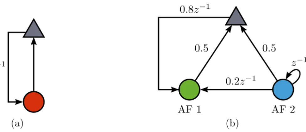
Figure 8: Example digraphs of combination topologies: (a) stand-alone adaptive filter; (b) arbitrary topology.
In the combination of AFs context, a topology is therefore a weighted digraph of degreeN+ 1 whose node set V includes a node for each component and oneoutput node that represents the output of the combination. They are differentiated by drawing the
former as circles and the latter as a triangle. Each arc in this digraph corresponds to a weighted transfer of the current coefficient vector. Explicitly, an arc with weight ω
exiting node n carries the coefficients ωwn,i. The a priori coefficients of a component is
evaluated by combining all arcs entering its node. For instance, consider the component
filters {m, n, p} connected by the arcs (m, p) and (n, p) with weights ωm and ωn. Such an arrangement is taken to mean wp,a =ωmwm,i+ωnwn,i. The arcs entering the output
node are combined in a similar fashion, but to form the current global coefficientswi.
These conventions are illustrated in Figure 8. Figure 8a shows a topology equivalent to a stand-alone AF for whichw1,a =wi−1 andwi =w1,i. An arbitrary topology is shown
in Figure 8b, wherew1,a = 0.8wi−1+ 0.2w2,i−1,w2,a =w2,i−1, and wi = 0.5w1,i+ 0.5w2,i.
Notice that when an arc is drawn unmarked its weight is considered to be one.
Clearly, not all digraphs represent topologies. Firstly, the digraph has to be weakly connected. If not, then at least one component filter cannot reach the output and can therefore be removed with no effect on the performance of combination. Repeating this procedure for all nodes disconnected from the output yield a weakly connected digraph
that forms a topology indistinguishable from the original one. Secondly, the in-degree of any node must be at least one. Indeed, if node n has a null in-degree, then wn,a = 0 always and the AF is restarted every iteration, which defies the recursive nature of these algorithms. Finally, when the topology is dynamic (changes withi), these requisites need
3.2.3
The parallel/incremental dichotomy
From Section 3.2.2, it is straightforward to see that even for combinations with a handful of component filters, the number of possible topologies is overwhelming. Hence, a direct approach to the study of these structures rapidly becomes intractable. However, two classes of topology have gained prominence in the literature, namely, the parallel and
incremental topologies [33, 35, 41, 73]. These categories can be distinguished in terms of the synchronicity of their components updates:
Definition 3.2 (Parallel topology). A topology is said to be parallel when the updates of its component filters can be evaluated simultaneously (synchronous components), i.e., when each component filter only depends on past information from other filters;
Definition 3.3 (Incremental topology). A topology is said to be incremental when the updates of its component filters depends on current data from previous filters (asyn-chronous components), i.e., component n depends on current information from compo-nentsm < n. In other words, the components are daisy-chained, as it is commonly said in electronics [82].
Separating topologies in only two classes may seem too restrictive at first, specially considering their number. However, it is usually the case that more complex configurations can be reduced to mixtures of these two categories. What is more, this dichotomy appears in several fields, from electrical circuits to data streaming (although sometimes under
dif-ferent names: parallel/series or parallel/serial). Specifically, the parallel/incremental di-chotomy is pervasive in numerical linear algebra and optimization algorithms used to solve problems similar to those found in adaptive filtering. These instances justify analyzing combinations only for purely parallel and purely incremental topologies.
Consider, for example, the problem of solving a linear system of equations, i.e., finding anx∈RM that satisfies
Ax=b, (3.2)
with A ∈ RN×M and b ∈ RN. Recall that this is the problem an adaptive algorithm is
which for the i-th iteration read
xm,i = 1
an bn−
n−1
X
p=1
anpxp,i−1−
N
X
p=n+1
anpxp,i−1
!
(Jacobi) (3.3a)
xm,i = 1
an bn−
n−1
X
p=1
anpxp,i−
N
X
p=n+1
anpxp,i−1
!
(Gauss-Seidel) (3.3b)
for an initial guess x0 and with A = [amn], b = [bm], and xi = [xm,i]. Indeed, the
Jacobi updates depend only on elements of xi−1 and therefore evaluates xi in a parallel
fashion. On the other hand, the Gauss-Seidel algorithm relies on the current value of some elements of x to updatexn,i, specifically {xp,i},p < n. Hence, it can only evaluate xi incrementally.
Another important pair of algorithms for solving (3.2) that gives rise to a
paral-lel/incremental dichotomy are known as row projection methods and are usually used to solve overdetermined systems (N > M). Their name comes from the fact that they operate on row slices of the original problem A = [ a1 a2 · · · aN ]T and b = [ bn ],
projecting candidate solutions onto the affine sets Hn = {x : anx =bi}. Depending on
whether the projections occur over allHnsimultaneously or sequentially, the technique is named Cimmino or Kaczmarz respectively [84]. Explicitly, definingPn as the projection
operator onto Hn,
xi = N
X
n=1
ηn[xi−1−2Pn(xi−1)] (Cimmino) (3.4a)
xi =PN
h
· · · P2[P1(xi−1) ]
i
(Kaczmarz) (3.4b)
with Pηn = 1 andηn>0.
The concept of sequential projections in (3.4) is also at the heart of a well-known solution to convex feasibility problems, which are found in adaptive algorithms such as the APA or set-membership (SM) filters [19]. Projection onto convex sets (POCS) methods are similar to row projection algorithms, but use arbitrary closed convex set instead of
simply the affine Hn [85]. POCS is also at the origin of proximal algorithms, which are heavily used in many areas of non-smooth convex optimization [86].
As a last example of parallel/incremental dichotomy, consider the case of a distributed optimization problem whose objective function can be decomposed as a sum of functions as in
h(x) =
N
X
n=1
where h, hn : RM →R. When solving (3.5) using gradient descent, two methods can be
derived depending on how the gradient of the fn is evaluated [72]
xi =xi−1−αi
N
X
n=1
∇hn(xi−1) (True gradient descent) (3.6a)
ψ0 =xi−1
ψn=ψn−1−αi∇hn(ψn−1), n = 1, . . . , N
xi =ψN
(Incremental gradient descent) (3.6b)
Notice that (3.6) is at the origin of some nomenclature used in the combination of AFs and ANs literature.
These examples, among many others, support the classification and analysis of com-binations in terms of parallel and incremental topologies.
3.3
The data reusing method
In the adaptive filtering literature, DR consists of either using K >1 times a single
data pair {ui, d(i)} or operating over a set of past data pairs {Ui,di}. Both techniques
have been successfully used to improve the performance of stand-alone AFs, albeit at the cost of increasing their complexity and memory requirements [87]. These algorithms are particularly appropriate in applications where data is intermittent, such as communication
systems, in which the rate of signaling is limited by bandwidth restrictions, or speech processing [87, 88]. Instead of idling between samples, the adaptive algorithm continues to operate over the available data to improve its estimates. Moreover, these AFs are able to trade off complexity and performance by choosingK, which is invaluable in many
scenarios [24].
Embedding DR in combinations of AFs is an important step towards formulating
high performance algorithms. Moreover, they allow most stand-alone DR AFs to be cast as combinations, providing new forms of analysis and generalization. In the context of combinations, however, differentiating between forms of data reuse is paramount. In fact, according to the definition for stand-alone AFs all combinations reuse data, since several
AFs operate over the data every iteration. The termsdata sharing and data buffering are therefore used to unambiguously refer to the different methods of reusing data.
and it remains by far the most common [33–36, 41–44, 59, 77, 89–96]. Overall, there is little advantage in using any other DR method when the input signal is white. The
addi-tional implementation and memory cost is unwarranted given the negligible performance gains [44, 45]. Correlated inputs, however, significantly degrade the convergence rate of combinations, specially when the component filters do not have input data decorrelating properties, such as the NLMS or the APA [18, 23, 25, 62, 71].
Data buffering combinations can be used to improve the transient behavior in that case. As in stand-alone adaptive filtering, this techniquebufferspast data pairs{ui−k, d(i− k)} into the rows of {Ui,di} and distributes them between the component filters. The
input buffer usually contains the lastK input samples, although this is not necessary. For instance, a buffer can be defined using k = {k′D : k′ = 0, . . . , K −1} for some constant D∈N, similar to [62]. More generally, k can be chosen from any size-K subset ofZ+.
An input buffer alone, however, does not fully specify a data buffering method, which
also needs to allocate a data pair to each component filter. Decouplingdata storage from data usage allows for more complex DR solutions than those usually found in stand-alone DR AFs [22, 87]. Indeed, the choice of protocols goes from the simple use of the n-th row of {Ui,di} by the n-th filter when N = K to randomized allocation of data pairs.
Moreover, this framework separates memory usage from algorithm complexity, something not found in stand-alone DR adaptive algorithms.
A last DR strategy worth mentioning isrefiltering. Here, output values from previous components are used as the input data of the current filter. These could be the actual output of the AFsyn(j) but also their output estimation errors en(j) or their coefficients
wm,j. For example, AFs in tandem use past error from other AFs as their desired signals,
i.e.,dn(i) = en−1(i−∆), for some delay ∆>0 [97]. Notice that, even if coefficient vectors
were used as inputs it would not incur in a topology change. The combination topology determines a connection between coefficients and has no relation to the data over which
the filters operate. Due to its lack of use, the remainder of this work considers only the data sharing and data buffering methods.
(a) (b)
(c) (d)
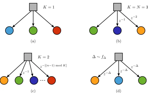
Figure 9: Data distribution networks: (a) data sharing; (b) stand-alone data reusing adaptive filter; (c) circular buffer; (d) randomized.
3.3.1
Data distribution networks
Data sharing and data buffering were described as two steps processes: first, data pairs are stored; then, data pairs are allocated to the component filters. Hence, one way of describing them is defining a set of indices K that determines a buffer from the data pairs{ui−k, d(i−k)}k∈K and a map between this buffer and the AFs. Naturally, the data
sharing case is trivial asK = 1 andK={0}for the buffer and all components get the same data pair. Notice, however, that what these steps effectively do is connect a data source to each filter in the combination. They can therefore be collapsed into a network that specifies how information reaches the component filters, i.e., a data distribution network. Such network can be described under the same formalism as combination
topolo-gies (Section 3.2), i.e., using weighted digraphs. To do so, define a node that represents the data source (denoted by a square). Then, using arcs as delay lines, connect this node to each component filter, effectively determining the data pair over which they operate and thus the DR strategy. Figure 9 illustrates the digraphs for data sharing (a) and the
data distribution method found in stand-alone DR AFs (b). Note that arcs only exit the data source node, which must always have an in-degree of zero. Three data buffering methods are presented below to illustrate the application of the proposed formalism.
Example 3.1(Circular buffer or barrel shifter). Using the data pair{ui−n−1, d(i−n−1)}
number of components in the combination to N = K. This limits the performance achievable by combinations, especially when less complex adaptive algorithms are used.
In [73], this issue was addressed by using a circular buffer (also known as abarrel shifter in the digital hardware milieu [82, 98]). Explicitly, the n-th component filter operates over the row k = (n−1) mod K of {Ui,di}. The data distribution network induced
by this method is illustrated in Figure 9c considering the buffer holds the K last data pair (K={0, . . . , K −1}). This method has been shown to improve the performance of incremental combinations to the point where they outperform the APA with considerably lower complexity [45, 47, 73].
Example 3.2 (Data selective distribution). Stand-alone data selective AFs (also known asset-membership, SM) are motivated by assuming that the additive noisev(i) is bounded and determining or estimating a feasibility set for the coefficient vector that meets the
corresponding error bound specifications [19]. These adaptive algorithms are more flexible in managing computational resources and have been successfully used in a myriad of applications [19, 99–101]. SM combinations can be obtained by using a data distribution network that only selects data pairs that yield errors larger than some threshold. In a
parallel combination whereN < K, for example, the strategy could allocate only the data pairs relative to the N largest errors.
Example 3.3 (Randomized data distribution). The row projection methods presented in Section 3.2.3 are intimately related to data buffering combinations of AFs. Indeed, parallel and incremental combinations operating over the rows of {Ui,di} are similar to
using Cimmino and Kaczmarz algorithms, respectively, on a system of equations such as
Uiwi = di. The Kaczmarz algorithm, in particular, operates sequentially over the rows
of this system, such that its performance may be affected by the order of the equations. To eliminate this undesirable effect, a randomized version of the Kaczmarz algorithm was proposed and analyzed in [102–104]. However, instead of selecting rows of Ui uniformly
at random, they are drawn with probabilities proportional to their Euclidian norms. One way to motivate this strategy is in terms of SNR improvements: in a system identification scenario, when the power of the regressorui fluctuates up, there is good chance that the
instantaneous SNR of the measurementsd(i) = uiw
o
+v(i) also increases.
A similar version of incremental combinations can be obtained by appropriately
choos-ing the distribution f∆ in Figure 9d. More complex strategies to select f∆ can also be
3.4
The supervisor
The supervisor or supervising rule is the element that evaluates the output of the combination (i.e., the mappingO in Definition 3.1). In other words, it is the part respon-sible for actually combining the AFs. It has therefore a significant effect on the overall performance of mixtures. Not surprisingly then, supervisors have attracted considerable
attention from the combinations of AFs community, lending their names to several struc-tures [33, 35, 91, 92, 106–108].
Supervising rules, however, are not a panacea. Other elements of the combination, such as the component filters and the topology, have as big an impact on its performance and can impose limitations to the effectiveness of the entire structure that the supervisor
cannot overcome. The convergence stagnation of parallel-independent combinations is a good example of such an issues and is investigated in details in Section 5.2.1.
The action of the supervisor over then-th component is represented by the supervising parameter ηn(i). Originally, the mapping O in Definition 3.1 does not define how these parameter are used to transform the AFs to the output of the combination. Section 3.2, however, restricted supervising rules to the class of linear combinations of coefficients to
make the description of topologies more concrete. Thus, this work considers the {ηn(i)} to be linear combiners and the output of the combination to be evaluated as,
wi = N
X
n=1
ηn(i)wn,i.
As far as supervisors go, this is by far the most common case, specially for parallel combinations [33, 35, 91, 92, 106–108]. A notable exception is the incremental supervisor used in [41, 43, 44].
Supervising rules, their characteristics, and constraints are intrinsically connected to the topology of the combination. They are therefore discussed in more details for the parallel (Chapter 5) and incremental (Chapter 6) cases separately. Nevertheless, their
adaptation methods can be classified in five broad categories:
• Statistical: some rules update the supervising parameters using a statistical method, such as Bayesian filtering or maximum a posteriori probability (MAP) [8]. They were more common in the earlier days of combinations of AFs [77, 93–95].
• Error statistics: this set of techniques relies on error statistics to update the su-pervising parameters. Usually, they are based on estimates of the global MSE, but instantaneous values and higher-order moments have also been used (e.g., [26, 27]).
The {ηn(i)} are sometimes evaluated using an activation function [35, 41, 44, 106].
• Stochastic gradient descent: inspired by individual AFs, stochastic gradient descent algorithms can be used to update the supervising parameters to minimize some cost function, usually the global MSE. This technique has been shown to be very effective and is ubiquitous in parallel combinations [33, 35, 39, 109, 110].
• Newton’s method (“normalized”): the normalized version of stochastic gradient de-scent rules were proposed to improve the robustness and reduce the variance of the supervising parameters. They are usually considered to be more effective than their unnormalized counterparts [39, 91].
3.5
An
FOB
illustration
To illustrate the use of Definition 3.1, an example FOB description is provided in this section. Even though the mappings used are fairly straightforward, they account for a comprehensive set of combinations, with different components, DR methods, supervi-sors, and topologies. Notable exceptions are combinations that employ refiltering and
incremental combinations supervised as in [41].
Explicitly, define the mappings
F : wn,i =wn,a+Hn,iUiTBn,ign(di−Uiwn,a) (3.7a)
O : wi =Ωiηi (3.7b)
B: Ωa = [ Ωi wi ]Zi−1, (3.7c)
wherewn,a is the n-th column of Ωa, Bn,i=bkbTk, bk is the k-th vector of the canonical
base of RK, Hn,i is an M ×M step size matrix, Z−1
i is an (N + 1)×N polynomial
matrix inz−1, theunitary delay, andη
i is theN×1 vector that captures the supervising
Before proceeding, notice that the adjacency matrix of the topology digraph is readily available from O and B (more specifically, ηi and Zi−1) in (3.7). Indeed, recall that the
topology digraph is akin to a mapping [ Ωi wi ]→[ Ωa wi−1 ], which can be derived
from (3.7) as
Ai = [ I ηi ]
"
Zi−1 0
z−1
#
. (3.8)
Note that Ai is iteration-dependent, which accounts for both dynamic topologies and
adaptive supervising rules.
In the sequel, example uses of (3.7) are presented to illustrate the versatility of FOB descriptions and suggest that some stand-alone adaptive algorithms can be cast as
com-binations of AFs, an avenue further investigated in Chapter 8. Without loss of generality, assumegn[x] =x and Hn=µnI, so that the components are all LMS filters.
Example 3.4(LMS+LMS with convex supervisor [33]).This combination can be written as
a(i) = a(i−1) +µae(i)[y1(i)−y2(i)]η(i)[1−η(i)]
η(i) = 1 1 +e−a(i)
wn,i=wn,i−1+µnuTi [d(i)−uiwn,i−1], n= 1,2
wi =η(i)w1,i+ [1−η(i)]w2,i,
(3.9)
with e(i) =d(i)−uiwi−1 and a(i)∈[−amax, amax].
Its FOB description is obtained from (3.7) using N = 2, K = 1, Mn =M,
Z−1 =
z−1 0
0 z−1
0 0
, and ηi =
"
η(i) 1−η(i)
# ,
where η(i) is evaluated as in (3.9). Note that despite its matrix form, F and B are equivalent to the recursion of two independent LMS filters.
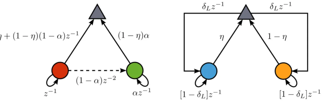
Example 3.5 (f{LMS + LMS} [42]). The LMS + LMS with cyclic coefficients feedback can be obtained by replacingwn,i−1 with wn,a in (3.9) and defining
wn,a =δL(i)wi−1+ [1−δL(i)]wn,i−1, (3.10)
where δL(i) = Pr∈Nδ(i−rL) is an impulse train of period L and δ(i) is the Kronecker
is now a function ofi. Explicitly,
Zi−1 =
1−δL(i) 0
0 1−δL(i)
δL(i) δL(i) z−1.
Indeed, Zi−1 represents the dynamic topology of a parallel combination with cyclic coef-ficients feedback.
Example 3.6 (TRUE-LMS [24, 25]). The TRUE-LMS is a stand-alone DR adaptive al-gorithm and is not usually considered a combination. Using (3.7) to describe its recursion
shows not only the versatility ofFOB descriptions, but also that this AF can be cast as a combination of LMS filters [73]. Indeed, the recursion of the TRUE-LMS, given in (2.11) as
wi =wi−1+µUiTei
can be described using (3.7) by choosingK =N, Bn,i=bnbTn, Mn=M,
Z−1 =
0 · · · 0 ... ... ... 0 · · · 0
z−1 · · · z−1
, and ηi =
1
N ·1,
where1 is a column vector of ones.
Example 3.7(DR-{LMS}N [73]). Fork= (n−1) modK, the data buffering incremental
combination of N LMS filters is given by [73]
w0,i =wi−1
wn,i=wn−1,i+µnuTi−k[d(i−k)−ui−kwn−1,i], n= 1, . . . , N
wi =wN,i.
It can be obtained from (3.7) usingMn =M and Bn,i=bkbTk, with k= (n−1) modK,
Z−1 = 0
I
...0 0 · · · 0
z−1 0 · · · 0
, and ηi =
0 ... 0 1 .
from [41] can be recovered.
3.6
Relation to adaptive networks
ANs consist of a collection of agents (nodes) with adaptation and learning capabili-ties that are linked through a topology and interact to solve inference and optimization
problems in a distributed and online manner. More specifically, each node estimates a set of parameters using an AF that operates on local data. Information from neighbor-ing nodes is aggregated by means of combination weights and also exploited by the local AF [3, 4, 6, 112–115].
This description resembles the ones for combinations of AFs presented in the beginning
of this chapter. They both involve a pool of AFs, each operating on individual data pairs, and some mixture of their estimates. ANs, however, are usually thought of as distributed entities, while combinations of AFs are considered local. Nevertheless, this need not be the case. An AN can be made of “virtual nodes” in a single processor, which is not
uncommon with graph algorithms applied to image processing [116]. Much the same way, the component filters of combinations can be physically distributed, as would be the case if the combination were implemented in a highly parallel processing framework such as Apache Spark [117].
There is, however, one important distinction between combinations of AFs and ANs:
their data source model. This is directly connected to their goal as signal processing algorithms. Combinations of AFs were proposed to improve the performance of adaptive algorithms and address issues such as transient/steady-state trade-off and robustness. Hence, just as stand-alone AFs, they operate over a single data source. On the other
hand, the goal of ANs is to solve distributed estimation and optimization problems, such as those in wireless sensor networks [79]. Therefore, they rely on different sources observed by different nodes. In a way, combinations of AFs are replacements for adaptive algorithms, whereas ANs use these adaptive algorithms to solve larger problems.
These observations suggest that the FOB description from Definition 3.1 can be applied to ANs with very little modification. The first important distinction is that, in
(a) (b)
Figure 10: FOB description of adaptive networks: (a) incremental and (b) diffusion.
instead of delayed versions of a single input{ui, d(i)}, the buffers Ui and di in (3.7) are
formed by observations from different sources. Explicitly, FOB descriptions of ANs can be derived from
F :wn,i=wn,a+µnuTn,i(dn(i)−un,iwn,a) (3.11a)
B:Ωa=ΩiZi−1, (3.11b)
where{un,i, dn(i)} is the data pair observed by node n. For clarity, only ANs with LMS nodes were considered. The use of (3.11) is illustrated in the examples below.
Example 3.8 (Incremental AN [3]). From a topology viewpoint, an incremental AN is similar to the incremental combinations from Example 3.7. Indeed, itsFOB description is derived from (3.11) using
Z−1 =
0
I
...
z−1 · · · 0
.
The digraph representing this combination can be found in Figure 10a. Notice that the
data distribution network now hasN data sources.
Example 3.9 (Diffusion AN [4]). An LMS adaptive diffusion network is described as2
ψn,i−1 =cnnwn,i−1+
X
ℓ∈Nn
cℓnwℓ,i−1 (3.12a)
wn,i=ψn,i−1+µnu∗n,i[dn(i)−un,iψn,i−1], (3.12b)
2
![Table 2: Classification as to the adaptive algorithm of the component filters AF LMS LMF RLS NLMS PNLMS LMS [2, 22, 25, 33–35, 39, 41, 42,44, 45, 47, 70, 73, 88–92, 96, 97, 106–108, 110, 118, 121– 123, 128–134] [26–28,90, 135,136] [34, 43, 110, 129] - -LM](https://thumb-eu.123doks.com/thumbv2/123dok_br/18462992.365318/55.892.194.739.168.683/table-classification-adaptive-algorithm-component-filters-nlms-pnlms.webp)