www.ann-geophys.net/26/3819/2008/ © European Geosciences Union 2008
Annales
Geophysicae
Significance tests for the wavelet cross spectrum and wavelet
linear coherence
Z. Ge
Ecosystems Research Division, NERL, USEPA, 960 College Station Road, Athens, GA 30605, USA Received: 9 July 2008 – Accepted: 21 October 2008 – Published: 2 December 2008
Abstract. This work attempts to develop significance tests for the wavelet cross spectrum and the wavelet linear coher-ence as a follow-up study on Ge (2007). Conventional ap-proaches that are used by Torrence and Compo (1998) based on stationary background noise time series were used here in estimating the sampling distributions of the wavelet cross spectrum and the wavelet linear coherence. The sampling distributions are then used for establishing significance levels for these two wavelet-based quantities. In addition to these two wavelet quantities, properties of the phase angle of the wavelet cross spectrum of, or the phase difference between, two Gaussian white noise series are discussed. It is found that the tangent of the principal part of the phase angle approxi-mately has a standard Cauchy distribution and the phase an-gle is uniformly distributed, which makes it impossible to es-tablish significance levels for the phase angle. The simulated signals clearly show that, when there is no linear relation be-tween the two analysed signals, the phase angle disperses into the entire range of[−π, π]with fairly high probabili-ties for values close to±πto occur. Conversely, when linear relations are present, the phase angle of the wavelet cross spectrum settles around an associated value with consider-ably reduced fluctuations. When two signals are linearly cou-pled, their wavelet linear coherence will attain values close to one. The significance test of the wavelet linear coherence can therefore be used to complement the inspection of the phase angle of the wavelet cross spectrum.
The developed significance tests are also applied to actual data sets, simultaneously recorded wind speed and wave ele-vation series measured from a NOAA buoy on Lake Michi-gan. Significance levels of the wavelet cross spectrum and the wavelet linear coherence between the winds and the waves reasonably separated meaningful peaks from those generated by randomness in the data set. As with
simu-Correspondence to:Z. Ge ([email protected])
lated signals, nearly constant phase angles of the wavelet cross spectrum are found to coincide with large values in the wavelet linear coherence between the winds and the waves. Not limited to geophysics, the significance tests developed in the present work can also be applied to many other quantita-tive studies using the continuous wavelet transform.
Keywords. Oceanography: physical (Air-sea interactions; Surface waves and tides) – General or miscellaneous (Tech-niques applicable in three or more fields)
1 Introduction
Perhaps the first one in geophysics, Liu (1994) defined the wavelet cross spectrum (WCS) between two time seriesx(t ) andy(t )as
Cxy(a, b)=X∗(a, b)Y (a, b), (1)
where a and b are scale and time variables, respectively, X(a, b)andY (a, b)are the wavelet coefficients of the time seriesx(t )andy(t ), respectively, and∗means complex con-jugate. In the definitions in Liu (1994) and TC98, the com-plex conjugate ofY (a, b), instead of that of X(a, b), was used. This inconsistency in definition will not affect any dis-cussions below. Equation (1) has defined a WCS for each point in the time-scale domain, similar to the wavelet power. Since the WCSCxyis complex when complex wavelets such
as the Morlet wavelet are used, its squared absolute value,
|Cxy(a, b)|2=|X∗(a, b)Y (a, b)|2=|X(a, b)|2|Y (a, b)|2, (2)
or simply its absolute value |Cxy(a, b)|, is often plotted
for visualisation (TC98). Apparently, a large value of
|Cxy(a, b)|2occurs when the two signalsxandyhave large
power at similar scales (frequencies) and around the same time, regardless of the local phase difference. When the phase information is desired, one needs to refer back to Eq. (1). Specifically, if the complex numberCxyis expressed
in terms of its module and phase angle, we have Cxy(a, b)= |X(a, b)|e−iθx(a,b)|Y (a, b)|eiθy(a,b)
= |Cxy|ei(θy(a,b)−θx(a,b)). (3)
This means that the phase angle of the WCS, i.e. θy(a, b)−θx(a, b), reflects the phase difference by which
y(t )leadsx(t )at the given scale and time. To present the information in phase Liu (1994) suggested that both the real and imaginary parts of the WCS be shown. Alternatively, another common practice is to show both the absolute value and the phase angle ofCxyin the time-scale domain.
A well-known disadvantage of the WCS in the time-scale domain is that it cannot be normalised to have a value bounded by, for example, zero and one. A normalisation similar to what brings about the correlation coefficient be-tween two time series always yields a value of unity for the WCS (TC98). In other words, the normalisation of the WCS cannot be done locally, and it must involve multiple points in the time-scale domain for some degree of smoothing. In geo-physics as well as other physical fields, a simple averaging in time will yield a useful measure of the local linear coupling in the scale (frequency) domain between two signals. This averaged quantity is referred to as the wavelet linear coher-ence (WLC) (or sometimes the wavelet coherency) expressed as
Lxy(a)= | R
T X∗(a, b)Y (a, b)db|2 R
T|X(a, b)|2db R
T|Y (a, b)|2db
, (4)
whereT is the time interval for averaging. Lxy is zero for
cases of no linear relation, is one for a perfect linear coupling,
and has values between zero and one for linear relations of different degrees. It is important to note that the linear rela-tion here is not exactly the same as the condirela-tions that result in a large value in the|Cxy|. A largeLxyat a particular scale
a results from persistently large wavelet energy densities at a in both time series and a nearly constant phase difference between these two series ataover a periodT. The numera-tor on the right side of Eq. (4) will otherwise have a near zero value. The role that the phase difference plays in the WLC will become clearer in Sect. 4.
The significance test, one of the central ideas in statisti-cal inference, is also important for the interpretation of re-sults using wavelet-based approaches. The significance test establishes significance levels below which the results are considered not to be “significantly” different from zero and hence none of them can be used with sufficient confidence. The null hypothesis (H0) in the present work will be based
The following discussions will be based on the Morlet wavelet, whose mother wavelet is defined as
ψ (t )=π−1/4eiω0te−t 2
2, (5)
whereω0 is set equal to 6.0 andt denotes time. The
fam-ily of the Morlet waveletsψa,b(t )can be generated by time
translations and scale dilations, such that ψa,b(t )=
1
√
aψ ( t−b
a ). (6)
The use of the Morlet wavelet and other complex wavelets will give rise to complex wavelet coefficients and hence ad-ditional information can be deduced from the phase angle of all complex wavelet quantities. The analyses in the follow-ing sections can readily be applied to other types of wavelets whenever the continuous wavelet transform is used. As for the significance tests on wavelet-based quantities obtained using the discrete wavelet transform, more considerations and manipulations are needed, which is beyond the scope of the present work.
2 Significance test of the wavelet cross spectrum
Two independent GWN series are denoted asx andy with variancesσx2andσy2, respectively. To avoid complication of notations, x andy also represent realisations of these two random processes.
The squared absolute value of the WCS of two GWNs is the product of two χ2-distributed random variables,
|X(a, b)|2and|Y (a, b)|2(Eq. 2). TC98 gave a form of the probability density function (PDF) of the absolute value (not squared) of the WCS:
fν(z)=22−νzν−1K0(z)/ Ŵ2(ν/2), (7)
whereŴis the Gamma function,K0(z)is the modified Bessel
function of order zero, and ν is the degree of freedom of theχ2distributions of the associated wavelet power. When complex wavelets are used, i.e.ν=2, Eq. (7) becomes
fTC(z)=zK0(z), (8)
where the subscript “TC” indicates that it results from TC98’s form Eq. (7). Equation (7), however, cannot be found in Jenkins and Watts (1968) as it seemed, nor was its deriva-tion clearly presented. In what follows, we will provide a clear derivation of the sampling distribution of the WCS of two GWNs.
Wells et al. (1962) obtained the probability distribution of the product of two independent non-central χ2-distributed random variables, also reviewed later by Kotz and Srinivasan (1969). The sampling distribution of|Cxy|2 based on two
independent GWNs is a special case where the degrees of
freedom of the twoχ2distributions are both 2 and the non-centrality parameters are both zero. More specifically, since
|X|2 δt σ2
x/2
∼χ22
and
|Y|2 δt σ2
y/2
∼χ22
withδt being the sampling period or the reciprocal of the sampling frequencyFs (Ge, 2007), their product
|X|2 δt σ2
x/2
|Y|2 δt σ2
y/2
∼W2,
whereW2denotes the probability distribution with a PDF
f (z)=1 2K0(z
1/2),
(9) based on Wells et al. (1962). Rearranging terms we have
|Cxy(a, b)|2
σ2
xσy2
∼ 1
4δt
2W
2. (10)
The significance level for a percentileαcan be deduced from the 1−αpercentile of theW2distribution. Moreover, we can
prove that the results obtained here, Eq. (10), and TC98’s form, Eq. (8), are equivalent to each other and are equally correct in determining the significance levels for the WCS of two GWNs. More details are given in Appendix A.
A set of simulated signals can be used to examine the proposed significance test of the WCS. Sine signals with a prescribed signal-to-noise ratio, SN, were generated. Same as those in Ge (2007), each of the signals consists of 2000 points with a sampling frequency of 50 Hz (i.e.δt=0.02 s). The entire period of 2000 points is divided into three inter-vals. In different intervals the two generated time series,x(t ) andy(t ), have different properties. The two signals are gen-erated such that
x =Asin(2πfxt )+GWN(0,1)
n∈ [701,900]
y =Asin(2πfxt+t (900t−t ()−700t (700) )2π )+GWN(0,1)
n∈ [701,900]
x =Asin(2πfxt )+GWN(0,1)
n∈ [901,1100]
y =Asin(2πfxt−23π )+GWN(0,1)
n∈ [901,1100]
x =Asin(2πfxt )+GWN(0,1)
n∈ [1101,1300]
y =Asin(2πfxt+23π )+GWN(0,1)
n∈ [1101,1300],
(11)
where n denotes the order of data points, fx is set at
0 2 4 6 8 10 12 0
0.002 0.004 0.006 0.008 0.01 0.012 0.014 0.016 0.018 0.02
freq (Hz)
variance (
σx 2σ
y
2)
b=150δ t b=300δ t b=450δ t 5% significance level
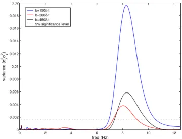
Fig. 1. Squared absolute value of the wavelet cross spectrum |Cxy(a, b)|2of two simulated signals given by Eq. (11) and the 5%
significance level.
SN=10 log10A2, and GWN(0,1) denotes a GWN with a
zero mean and a unit standard deviation. These two simu-lated signals thus have a linearly varying phase difference in the first interval n∈[701,900], a constant phase difference
−2π/3 in the second intervaln∈[901,1100], and a constant phase difference 2π/3 in the third intervaln∈[1101,1300]. The signals in the periods prior ton=701 and aftern=1300 are just GWNs. TC98’s Fortran code for estimating the wavelet coefficient was used with an adjustment as suggested in Appendix A of Ge (2007). To avoid the cone of influence (TC98), only the central 600 points (n∈[701,1300]) are used for analysis. Although the retained wavelet coefficients still are affected by the edge effect at the largest scales, the influ-ence of the edges is negligible.
Figure 1 shows the squared absolute value of the WCS,
|Cxy|2, between the simulated signalsx andy (Eq. 11)
nor-malised by the product of the variances of the two signals over the period that covers the central 600 points. The three curves in Fig. 1 represent three vertical slices of|Cxy|2
val-ues in the original time-scale domain, with scaleaconverted into frequencyf through the relation
a=fc/f ≈0.9394/f (12)
for the Morlet wavelet. The timing for the three curves,b, is expressed relative to the beginning of the central 600 points instead of that of the entire 2000 points. Hence, the times at b=150δt,b=300δt, andb=450δt fall in the three intervals in Eq. (11), respectively. With a relatively high SN ratio, all the three curves of|Cxy|2are well above the theoretical
5% significance level based on Eq. (10), regardless of the patterns of the phase difference betweenxandy in different intervals. As expected, all the three curves peak at about 8 Hz (i.e.fx) with small deviations due to the added GWNs.
Very small ripples are observed in Fig. 1 at frequencies lower than 4 Hz. These ripples are correctly indicated to be random noise, or not significantly different from zero with a 95% confidence, by the 5% significance level.
3 Property of the phase angle of the WCS
The phase angle of the WCS for each point in the two-dimensional time-scale domain can be plotted (TC98). TC98, however, did not propose any significance test or con-fidence interval for the phase. The significance test on the phase angle appears not to be as important as that on other popular wavelet-based quantities. Nevertheless, some of the properties of the phase angle of the WCS might be interesting to the users of the wavelet analysis.
If the range of the phase angleφis[−π, π]and the con-ventional range of the arctangent function is[−π/2, π/2], we have
φ=arctanI m[X ∗Y]
Re[X∗Y] +µπ=φ0+µπ, (13) whereµ=0 when the complex numberCxy=X∗Y is in the
first or fourth quadrant of the complex plane,µ=1 whenCxy
is in the second quadrant, and µ=−1 whenCxy is in the
third quadrant. Using the real and imaginary parts ofXand Y, Eq. (13) leads to
tanφ0=
Re[X]I m[Y] −I m[X]Re[Y]
Re[X]Re[Y] +I m[X]I m[Y]. (14) Whenx andy are independent GWNs, the numerator and the denominator of Eq. (14) are independent of each other, unbounded, and can take any real values. As suggested by Jenkins and Watts (1968, p. 366), they can be considered to be approximately normally distributed variables. The quan-tity tanφ0is thus the ratio of two normally distributed
ran-dom variables, which has a standard Cauchy distribution de-noted asC(0,1). More details are given in Appendix B. The PDF of tanφ0is therefore
f (z)= 1
π(1+z2), (15)
which yields no mean or any higher-order moments but a zero median. That Cauchy distributed random variables have no variance implies that the random variable can take ex-treme values more often than would naturally occur (e.g. for normally distributed variables). Given a sufficiently long set of time seriesx andy (GWNs), tanφ0can disperse into an
unbounded range with extreme values observed more fre-quently than rarely. The angleφ0can hence take any value
between−π/2 and π/2 and is distributed much more uni-formly than a normally distributed variable. Papoulis (1965, p. 199) reached a further result: φ0in Eq. (14), as the
that has independently normally distributed real and imagi-nary parts with zero means and equal variances, has an ex-actly uniform distribution in the interval from−π/2 toπ/2. Taking advantage of this observation as well as the fact that Cxy=X∗Y can be in the four quadrants of the complex plane
with equal probabilities, we deduce that the phase angle of Cxy=X∗Y,φ, has a uniform distribution in the interval
be-tween−π toπ. Therefore, no significance level can be es-tablished with the aid of the sampling distribution ofφ. In other words, the phase angleφ will fill the range between
−πandπwithout concentrating around any particular value. The randomness of the two GWNs x and y makes φ not likely to be bounded around any value but rather scattered in the whole range of[−π, π].
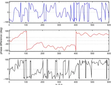
Figure 2 shows the time variation of the phase angleφof the WCS of the simulated signalsx andygiven by Eq. (11) at three frequencies: 6 Hz, 8 Hz, and 10 Hz. According to Eq. (11) the phase at 6 Hz and 10 Hz should reflect both ran-domness due to the added GWN components and the influ-ence of the scale at 8 Hz through the correlation between ad-jacent scales. The phase pattern at 8 Hz is evident, including a linear increase in the first 200-point period, a relatively sta-ble negative phase angle in the middle 200-point period, and a nearly constant positive phase angle in the last portion of the period. However, the nearly constant phase angles in the second and third intervals are not exactly−2π/3 and 2π/3 as prescribed by Eq. (11). This is not completely unexpected since the phase difference betweenx andy (Eq. 3) at any frequency has been perturbed by the different GWN compo-nents added tox andy. Affected by the scale at 8 Hz, the phase angle of the WCS at 10 Hz bears resemblance to that at 8 Hz, while the pattern of the phase appears to be much more irregular. The phase angle at 6 Hz reflects randomness with values close to±π occurring more often than rarely, especially within the interval of the last 200 points. The dif-ference between the phase patterns at 8 Hz and those at 6 Hz and 10 Hz are consistent with the deduced properties of the phase angle of the WCS of two GWNs. It hence appears that if the phase difference between two signals has a regu-lar pattern the phase of the WCS tends to become stable and reveal that pattern rather than fluctuate everywhere. The sig-nificance test of the phase angle of the WCS should thus be replaced by identification of regular phase patterns. Since it is still quite subjective to distinguish a regular phase pattern from randomly fluctuating ones, we suggest that the wavelet linear coherence of the same two signals be inspected. More details are given in Sect. 4.
4 Significance test of the wavelet linear coherence The definition of the WLC is given by Eq. (4). For a certain a, the discrete form of Eq. (4) can be expressed as
Lxy(a)= | P
mXa∗(b)Ya(b)|2 P
m|Xa(b)|2Pm|Ya(b)|2
, (16)
0 100 200 300 400 500 600
−180 0 180
0 100 200 300 400 500 600
−180 −60 0 60 180
phase difference (deg)
0 100 200 300 400 500 600
−180 0 180
b (δ t)
Fig. 2. Phase angle of the wavelet cross spectrum, φ (a, b)
(φ∈[−π, π]), of two simulated signals given by Eq. (11) at 6 Hz
(blue), 8 Hz (red), and 10 Hz (black).
where the summations are over m data points such that T=mδt. This form of the WLC can be readily viewed as a squared correlation coefficient between twom-point time series:
Xa∗ and{Ya}. As Jenkins and Watts (1968, p. 379)
pointed out, the sampling distribution of the correlation co-efficient (not squared) of two normally distributed random variables can be obtained by Fisher’s z-transformation. Then the only problem to consider now is how the two series,Xa∗ and{Ya}, can be treated as realisations of two random
vari-ables.
The continuous wavelet transform as used in the present work gives rise to redundancy when one-dimensional time series is resolved into a two-dimensional time-scale do-main. Neither of the two series,
X∗a(j ) and {Ya(j )}
(j=1,2,· · ·, m), can be considered to be a series of inde-pendent observations unless the inter-correlation of adjacent data points in
Xa∗ and{Ya}is removed. It can be deduced
that the covariance of two wavelet coefficients of a GWN se-riesxat scaleaand timesbi andbj, i.e.
|Cov[Xa(bi), Xa(bj)]| =δt σx2e−1b 2/4a2
, (17)
where1b=|bi−bj| (Appendix C). The decay of the
corre-lation coefficient of wavelet coefficients of the same scale with a separation in time1bis determined by the exponen-tial functione−1b2/4a2, or
ρ(1b)=e−1b2/4a2 (18)
withρ(1b) denoting the absolute value of the correlation coefficient of temporally adjacent wavelet coefficients. Ob-viously, farther apart wavelet coefficients are less correlated. More discussion can be found in Appendix C.
−3 −2 −1 0 1 2 3 4 5 6 7 −0.8
−0.6 −0.4 −0.2 0 0.2 0.4 0.6 0.8
t
ψ
(t)
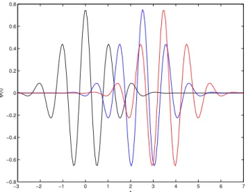
Fig. 3.Decorrelation of wavelet coefficients of a GWN with an in-creasing time separation reflected by the decorrelation of wavelets.
The mother Morlet waveletsψ (t )are used for illustration. The blue
and the black wavelets have a correlation coefficient of 1/5 (κ=5);
the red and the black wavelets have a correlation coefficient of 1/20
(κ=20).
for1b we are able to determine the time separation1b be-yond which the correlation coefficient between wavelet co-efficients falls below 1/κ. The decorrelation parameter κ can be set at a large positive number such as 5 or 20, cor-responding to correlation levels of 1/5 or 1/20, respectively. We can further assume that the wavelet coefficients are con-sidered to be independent of each other when their correla-tion coefficient is below 1/κ. In this approach, a series of wavelet coefficients, such as
Xa∗(j ) (j=1,2,· · ·, m), can be grouped into a number of independent sub-series. Within any individual sub-series the correlation coefficient of any two wavelet coefficients is larger than 1/κ, while the wavelet coefficients belonging to different sub-series have a correla-tion coefficient lower than 1/κ. Therefore, each sub-series is equivalent to an independent observation in a sample, and the number of the sub-series is equivalent to the sample size. More specifically, settingρ(1b)=1/κ yields
1b=2√lnκa. (19)
The sample size, denoted asN (a)which is a function of the scale, can be estimated through the relationN (a)=T /1b, so that
N (a)= mδt
2√lnκa. (20)
Since the correlation coefficient of the wavelet coefficients of a GWNy decays at the same rate as described by Eq. (18), Eq. (20) is also applicable to the wavelet coefficient ofy. For example, for the case ofa=1 (the mother Morlet wavelet), the time separation1bforκ=5 is 2√ln 5 and that forκ=20
is 2√ln 20. The Morlet wavelets with these two separations from a Morlet wavelet at the origin are shown in Fig. 3, giv-ing an idea about how wavelet coefficients become decor-related as they are more and more separated in time. The correlation coefficient of wavelet coefficients essentially is reflected by that of wavelet functions when the analysed time series is a GWN (Appendix C). For clarity, the Mor-let waveMor-lets (real part), instead of the waveMor-let coefficients, are shown in Fig. 3. Figure 3 also indicates that increasing κ from 5 to 20 does not require a much wider separation. Hence, we will simply setκat 5 for most cases in the follow-ing sections.
The two original seriesXa∗ and{Ya}of lengthmcan now
be treated as two reduced series of independent observations of lengthN (a). Using Fisher’s transformation we have
arctanh(rxy)∼N (arctanh(ρxy),
1
√
N (a)−3), (21) whererxy andρxy are the theoretical and estimated
corre-lation coefficients of
Xa∗ and{Ya}. In the case of x and
y being GWNs and a large N (a) (i.e. at reasonably small scales), the probability distribution is approximately
arctanh(rxy)∼N (0,
1
√
N (a))≈N (0,
s
2√lnκa
mδt ). (22) Theαsignificance level of the WLC is hence
Dα(Lxy)=tanh2
sα s
2√lnκfcFs
mf
(23)
withsα denoting the 1−αpercentile of the standard normal
distribution and scales converted into frequencies through Eq. (12). More detailed derivation can be found in Ap-pendix C. WhenN (a)is close to or even smaller than 3, as is often the case at very large scales, the resultingα signifi-cance level according to Eqs. (21) and (22) tends to be larger than one. For most cases, therefore, no WLC results should be trusted with confidence at the largest scales.
Van Milligen et al. (1995) estimated the “statistical noise level” of the WLC as
DV M(Lxy)≈2 s
Fs
mf (24)
through a similar but much more heuristic reasoning. We be-lieve that their so-called statistical noise level is exactly the significance level, but it is not clear whatαvalue was asso-ciated with Eq. (24). Comparing Eqs. (23) and (24) we have an impression that Eq. (23), with more factors taken into ac-count, is a much more accurate form than the one suggested by van Milligen et al. (1995).
0 5 10 15 20 25 0
0.1 0.2 0.3 0.4 0.5 0.6 0.7 0.8 0.9 1
freq (Hz)
Lxy
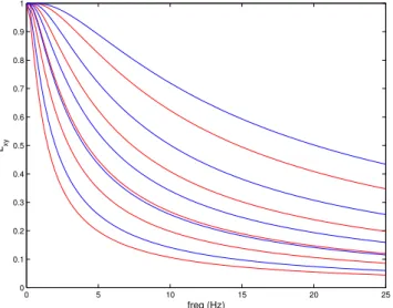
Fig. 4.5% significance levels of the wavelet linear coherence: red:
κ=5,m=40, 80, 140, 200, and 400 from top to bottom; blue:κ=20,
m=40, 80, 140, 200, and 400 from top to bottom.
ofκ=20. It is obvious that the low frequency range tends to be seriously affected by random noise, and the significance levels drop rapidly with increasingm. When the decorrela-tion condidecorrela-tion is relaxed toκ=5, the resulting significance levels (the red set of curves) are evidently, but not consid-erably, lower than their corresponding ones forκ=20. For example, form=80, the difference of the significance levels betweenκ=20 andκ=5 is approximately 0.08 for most of the frequencies. The difference seems to be much smaller whenmis increased to 200 or 400. In most practical cases, therefore,κ=5 should be reasonably effective. Another fea-ture of Fig. 4 is that all significance level curves are below one. This is not realistic because Eq. (23) is only applicable to scales that are not too large. One should be aware of the possibility ofN (a)being close to 3, and, practically, should not make use of any results below 5 Hz in Fig. 4.
Figure 5 shows three WLC curves starting at b=50δt, 250δt, and 450δtwith an integration lengthmof 120 points (κ=5), so that the three WLC curves are completely esti-mated within the three intervals respectively. In Fig. 5, the WLC levels around 8 Hz for the second and third intervals are well above the local 5% significance level, while that for the first interval cannot be distinguished from the WLC caused by random noise. This clearly exhibits the effect of the phase-difference pattern ofxandyon the resulting WLC values. During the second and third intervals, the stability in the phase difference (Fig. 2) yields a peak in the WLC at the associated frequency. In contrast, the linearly varying, i.e. inconstant, phase difference betweenxandy in the first in-terval leads to a low level of WLC that is considered not to be significantly larger than zero. Furthermore, the rapid fluctua-tions at low frequencies, which have obviously resulted from randomness, are collectively far below the 5% significance
0 2 4 6 8 10 12
0 0.1 0.2 0.3 0.4 0.5 0.6 0.7 0.8 0.9 1
freq (Hz)
Lxy
Fig. 5.Wavelet linear coherenceLxyof two simulated signals given
by Eq. (11) estimated over m=120 points starting fromb=50δt
(blue),b=250δt(red), andb=450δt(black). The three WLC curves
represent, respectively, the linear relations in the three intervals as in Eq. (11).
level, especially from 1 Hz to 5 Hz. This implies the possi-bility of relaxingαto larger values, such as 10% or 20%, for this particular case.
5 Significance tests on actually observed data sets
As pointed out previously, theoretically developed signifi-cance tests should be examined and validated by actually observed data, simply because assumptions, simplifications, and approximations have been inevitably made in the course of derivation. The NOAA’s (National Oceanic and Atmo-spheric Administration) Lake Michigan wind-wave data set is used here again. The description of the data set can be found in Ge and Liu (2007 and 2008) and Ge (2007). Briefly, the horizontal wind velocity time series (denoted as u) and the wave elevation (denoted as η) were simultane-ously recorded by a NOAA 3-m discus buoy, deployed dur-ing the autumn of 1997 in nearshore eastern Lake Michigan of the United States (43.02◦N, 86.27◦W) with a sampling frequencyFs=1.7 Hz. The data set exhibits a long process
of wave growth in response to increasing wind forcing, as discussed previously by Ge and Liu (2008).
A 2000-point data segment was picked out from the wind-wave data set, and the central 600-point wind-wavelet coefficients were used for further analysis. The WLCLηuestimated over
0 0.1 0.2 0.3 0.4 0.5 0.6 0
0.1 0.2 0.3 0.4 0.5 0.6 0.7 0.8 0.9 1
freq (Hz)
Lη
u
wavelet linear coherence η − u 5% significance level 20% significance level
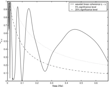
Fig. 6. Wavelet linear coherence of the wave elevation η and
the wind velocity fluctuationsu estimated over the period from
b=200δt tob=299δt (m=100), compared with the 5% and 20%
significance levels.
0.35 Hz to 0.65 Hz in which all frequency components in the winds are linearly coupled with those in the waves, because the width of this peak should not be the consequence of lo-cally poor resolution in frequency. A third peak at 0.07 Hz is also above the 5% significance level with a high WLC value of 0.94. Since the local significance level is almost equally high (about 0.84), we do not consider this peak to be statisti-cally significant.
The phase difference between the wave and wind time series, or the phase angle of their WCS Cηu at three
rep-resentative frequencies, 0.15 Hz (for extremely high WLC), 0.28 Hz (for extremely low WLC), and 0.5 Hz (for locally high WLC), is shown in Fig. 7. Fromb=200δtto 299δt, the phase difference at 0.15 Hz is very stable around±180◦(note that the large steps are artificially caused by the definition of the phase angle), indicating that the wind and wave time se-ries are almost perfectly out of phase at 0.15 Hz during the time period from b=200δt to 299δt. This characteristic is however not as evident in other time periods. At 0.5 Hz in the same period, the phase difference also appears to be centered around 180◦, while its deviation from 180◦is relatively larger than that at 0.15 Hz (e.g. fromb=230δt to 260δt). In com-parison, the phase difference in the same period at 0.28 Hz exhibits a much more random pattern. The phase angle does not seem to settle around any particular value. The different characteristics of the phase angle at these three frequencies in the studied 100-point period are consistent with the de-duced properties of the phase angle of the WCS and its re-lation to the WLC in the previous sections. Consequently, a significance test of the WLC can be used to help identify meaningful patterns in the phase angle of the WCS.
0 50 100 150 200 250 300 350 400 450 500
−180 0 180
0 50 100 150 200 250 300 350 400 450 500
−180 0 180
phase difference (deg)
0 50 100 150 200 250 300 350 400 450 500
−180 0 180
b (δ t)
Fig. 7. Phase angle of the wavelet cross spectrumCηu at 0.15 Hz
(blue), 0.28 Hz (red), and 0.5 Hz (black). Wide curves of all colors
highlight the period fromb=200δttob=299δt.
Figure 7 also reveals the randomness and intermittency of the phase angle. During the period fromb=50δt to 150δt, for example, the wind velocity fluctuations lead the wave elevation by a linearly varying phase angle growing from
−180◦to 180◦from 50δtto 100δt and then growing from 0 to 180◦from 110δtto 150δtat 0.15 Hz. At 0.28 Hz and in the same interval, however, the winds appear to lead the waves by a relatively constant phase angle of approximately 90◦, which is only briefly interrupted by a sharp peak at around b=100δt. According to Sect. 4, this pattern implies a rela-tively high WLC value over that period. At 0.5 Hz, the winds lag behind the waves by about 160◦in most part of the same period, while from b=100δt to 120δt the phase difference between the winds and the waves is slightly larger than 180◦, so that the angle wraps around and appears to be+180◦.
6 Conclusion
Interpretation of results using wavelet-based techniques then should be done in the same manner as for statistical infer-ence.
On the other hand, significance testing on wavelet-based quantities (now treated as wavelet-based “statistics”) can be extremely difficult, because the wavelet analysis is most fre-quently used for processing nonstationary time series. When using sampling distributions based on background noise time series to establish the null hypothesis, we are clear that the choice of the background noise signals can be subjective and arbitrary. Instead of examining an exhaustive list of back-ground noise series, the present work is focused on a rep-resentative combination, two independent Gaussian white noise series. Sampling distributions of the WCS and the WLC of two independent GWN series are estimated through rigorous statistical reasoning. When other combinations of reference series are preferred, the same procedure can be followed to obtain their associated sampling distributions. Significance levels of these two wavelet-based quantities are then deduced based on the sampling distributions.
In the present work, the sampling distributions of the WCS and the WLC are derived by analytical approaches, which are preferred by TC98. In many cases where the analyt-ical approach seems to be difficult, Monte Carlo tions can be employed (TC98). The Monte Carlo simula-tion, however, has disadvantages of high computation cost and the inability to provide the user with a clear mathemat-ical form for the sampling distributions or the significance levels. Through simulated noisy sinusoidal signals and ac-tual wind-wave time series observed from Lake Michigan, it is shown that the analytically developed significance tests are reasonably effective in distinguishing large WCS and WLC values that indicate meaningful linear spectral relations from those generated by random noise. Furthermore, in the ab-sence of significance tests for the wavelet phase difference between time series (i.e. the phase angle of the WCS), the significance test of the WLC can help identify meaningful patterns in the phase difference. In contrast to earlier appli-cations of the wavelet analysis (e.g. Foufoula-Georgiou and Kumar, 1994), significance tests help to place the interpreta-tion of results on a rigorous statistical basis, so that the in-terpretation no longer depends on the researcher’s personal experience and judgment.
Significance tests of third-order wavelet spectral moments, such as the wavelet bispectrum and the wavelet bicoherence (van Milligen, 1995; Ge and Liu, 2007; Elsayed, 2008), will be investigated in a future work.
Appendix A
Sampling distribution of the WCS given by TC98
According to Eq. (10), the α significance level of
|Cxy(a, b)|2/σx2σy2 is δt2Z(1−α)/4, where Z(1−α) is the
1−αpercentile of theW2 distribution. Alternatively, since
the conventionally defined wavelet coefficient of x(t ) at time b and scale a, i.e. X(a, b), and the wavelet coeffi-cient of x(t ) at time tn and scale a defined by TC98, i.e.
Wnx(a), are related by|X(a, b)|2=δt|Wnx(a)|2(Ge, 2007) (a similar relation holds fory(t )), the α significance level of
|Wnx(a)Wny(a)|2/σx2σy2 becomes Z(1−α)/4. Therefore the
αsignificance level of|Wnx(a)Wny(a)|/σxσyis
√
Z(1−α)/2. Compared with TC98’s result that the α significance level of|Wnx(a)Wny(a)|/σxσyisZT C(1−α)/2 for GWNsxandy
and complex wavelets (ν=2) withZT C(1−α)denoting the
1−αpercentile of the distribution given by Eq. (8), the only question now remaining is whether ZT C(1−α)is equal to
√
Z(1−α). We only have to consider two PDFs: Eq. (8) given by TC98 without any explanation and Eq. (9) as a par-ticular case of the results given by Wells et al. (1962).
The cumulant probability functions (CDF) can be obtained from Eqs. (8) and (9), respectively. The CDF based on TC98’s form is
FT C(z)=1−zK1(z) (A1)
and the CDF associated with the PDF given by Eq. (9) is
F (z)=1−√zK1(√z) (A2)
for any real positive z. It is obvious immediately that ZT C(1−α)=√Z(1−α)holds for anyα value from zero to
one. TC98’s forms, Eqs. (7) and (8), are hence reconciled with Eq. (9) developed in the present work.
Appendix B
More details on the sampling distribution of the phase angle of the WCS
A property will be useful for the following discussion: if two time series (more rigorously, random variables or stationary random processes) are independent, the mean value of their product is the product of their respective means, i.e.
E[xy] =
Z Z
xyf (x, y)dxdy
=
Z Z
xyf (x)f (y)dxdy
=E[x]E[y], (B1)
where E[· · ·] means the expectation, f (x, y) denotes the joint probability density function ofx andy, andf (x)and f (y)are the marginal probability density functions ofx and y, respectively.
From Eq. (14), tanφ0is the ratio of
−100 −8 −6 −4 −2 0 2 4 6 8 10 0.05
0.1 0.15 0.2 0.25 0.3 0.35
z
probability density
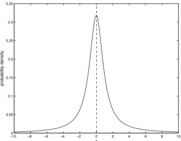
Fig. B1.Probability density function of the standard Cauchy
distri-butionC(0,1).
they can be approximately treated as normally distributed variables. Following the same approach that leads to the independency of the real and imaginary parts of the wavelet coefficient of a GWN (Ge, 2007), we have the independency between any two of Re[X], I m[X], Re[Y], and I m[Y]. Therefore, also using Eq. (B1),
E[A] =E[Re[X]I m[Y]] −E[I m[X]Re[Y]]
=E[Re[X]]E[I m[Y]] −E[I m[X]]E[Re[Y]] =0, and similarlyE[B]=0. Hence,
Var[A] =E[A2]
=E[Re2[X]I m2[Y] +I m2[X]Re2[Y]
−2Re[X]I m[Y]I m[X]Re[Y]]
=E[Re2[X]]E[I m2[Y]] +E[I m2[X]]E[Re2[Y]]. SinceRe[X],I m[X],Re[Y], andI m[Y]of GWNx andy all have zero means,
Var[A] =Var[Re[X]]V ar[I m[Y]] +Var[I m[X]]Var[Re[Y]], which yields
Var[A] = 1 2δt
2σ2
xσy2. (B2)
Similarly,Bhas the same variance. With zero means, their covariance Cov[A, B] =E[AB]
=E[(Re[X]I m[Y]
−I m[X]Re[Y])(Re[X]Re[Y]
+I m[X]I m[Y])].
Expanding the right side of the equality above and using the properties ofRe[X],I m[X],Re[Y], andI m[Y], we have
Cov[A, B] =0. (B3)
Therefore, the two random variables,AandB, both have an approximately normal distributionN (0, δt σxσy/
√
2)and are independent of each other. Their ratio, tanφ0, has a standard
Cauchy distributionC(0,1), whose PDF is expressed as f (z)= 1
π(1+z2)
and is shown in Fig. B1. The PDF of the Cauchy distribu-tion in Fig. B1 has a sharp peak at the origin and quite heavy tails at positive and negative ends. Because of the slow decay of the PDF values at large positive and negativez, integrals such asR∞
−∞z
nf (z)dzdo not exist in the real domain. The
Cauchy distribution hence has no moments of any order, not even a mean value. Zero is obviously its median, but a me-dian is not meaningful in determining its significance levels or confidence intervals. One might also attempt to estimate the integrals, such asRz0
−z0f (z)dzand R∞
z0 f (z)dz, to deter-mine the critical valuez0for establishing an associated
sig-nificance level. In fact, however, neither of them converges in the real domain. For example, we have
Z ∞ z0
dz π(1+z2)=
1
2π[π+i(ln(1+z0i)−ln(1−z0i))], which is not a real number unlessz0=0, a trivial case.
Appendix C
More details on the sampling distribution of the WLC
First of all, more detailed derivation of Eq. (17) is given. De-noting the wavelets evaluated at(a, bi)and(a, bj)as ψa,i
andψa,jrespectively, we have
Cov[Xa(bi), Xa(bj)]
=Cov
Z
x(t )ψa,i∗ (t )dt,
Z
x(t )ψa,j∗ (t )dt
=E
Z
x(t )ψa,i∗ (t )dt
Z
x(t )ψa,j∗ (t )dt
due to the zero-mean property. Therefore, Cov[Xa(bi), Xa(bj)]
=E
Z Z
x(t )x(t′)ψa,i∗ (t )ψa,j∗ (t′)dt dt′
=
Z Z
E[x(t )x(t′)]ψa,i∗ (t )ψa,j∗ (t′)dt dt′
=δt σx2
Z
ψa,i∗ (t )ψa,j∗ (t )dt.
Taking the absolute value of both sides of the equation above,
|Cov[Xa(bi), Xa(bj)]| =δt σx2| Z
In Ge (2007) it was defined thatI2=|R ψa,i(t )ψa,j(t )dt|2,
and hence
|Cov[Xa(bi), Xa(bj)]| =δt σx2 p
I2. (C2)
Using the results in Ge (2007) that I2=e−1b
2/2a2
with1b=|bi−bj|, we reach Eq. (17).
Moreover, since
Var[X(a, b)] =Var[Re[X] +iI m[X]]
=Var[Re[X]] +Var[I m[X]], using results in Ge (2007) we obtain
Var[X(a, b)] =δt σx2. (C3)
Comparing Eqs. (17) and (C3), we immediately have ρ(1b)=e−1b2/4a2
= |
Z
ψa,i∗ (t )ψa,j∗ (t )dt|,
i.e. Eq. (18), where ρ is the correlation coefficient of the wavelet coefficients that are separated by1b. Particularly, when1b=0,ρ(0)=1.
Furthermore, Eq. (C1) indicates that the covariance of two wavelet coefficients of a GWN that are separated in time is determined by the integral|R
ψa,i∗ (t )ψa,j∗ (t )dt|. This inte-gral can be viewed as the covariance of two wavelets, one at (a, bi)and the other at(a, bj). Noting that when1b=0 the
integral becomes
|
Z
ψa,i∗ (t )ψa,i∗ (t )dt| =pI2|1b=0=1,
this kind of covariance has the same properties as the ab-solute value of a correlation coefficient. Consequently, the correlation coefficient between wavelet coefficients,ρ(1b), can be expressed as the correlation coefficient between two wavelets that are at the same locations as their associated wavelet coefficients in the time-scale domain. This justifies the use of wavelets in Fig. 3 to show the decorrelation of wavelet coefficients with an increasing time separation.
Acknowledgements. The author wishes to thank the Ecosystems
Research Division of the USEPA (NERL) and the Research Asso-ciateship Programs of the National Research Council for their re-sources and financial support.
Topical Editor S. Gulev thanks C. Torrence and another anony-mous referee for their help in evaluating this paper.
References
Elsayed, M. A. K.: Nonlinear wave-wave interactions, J. Coastal Res., 24, 798–803, 2008.
Foufoula-Georgiou, E. and Kumar, P. (Eds.): Wavelets in Geo-physics, Academic, San Diego, 1994.
Ge, Z.: Significance tests for the wavelet power and the wavelet power spectrum, Ann. Geophys., 25, 2259–2269, 2007, http://www.ann-geophys.net/25/2259/2007/.
Ge, Z. and Liu, P. C.: A time-localized response of wave growth process under turbulent winds, Ann. Geophys., 25, 1253–1262, 2007, http://www.ann-geophys.net/25/1253/2007/.
Ge, Z. and Liu, P. C.: Long-term wave growth and its linear and nonlinear interactions with wind fluctuations, Ann. Geophys., 26, 747–758, 2008,
http://www.ann-geophys.net/26/747/2008/.
Grinsted, A., Moore, J. C., and Jevrejeva, S.: Application of the cross wavelet transform and wavelet coherence to geophysical time series, Nonlin. Processes Geophys., 11, 561–566, 2004, http://www.nonlin-processes-geophys.net/11/561/2004/. Jenkins, G. M. and Watts, D. G.: Spectral analysis and its
applica-tions, Holden-Day, San Francisco, 1968.
Kotz, S. and Srinivasan, R.: Distribution of product and quotient of Bessel function variates, Ann. I. Stat. Math., 21, 201–210, 1969. Liu, P. C.: Wavelet spectrum analysis and ocean wind waves, Wavelets in Geophysics, edited by: Foufoula-Georgiou, E. and Kumar, P., Academic, San Diego, p. 151–166, 1994.
Lundstedt, H., Liszka, L., Lundin, R., and Muscheler, R.: Long-term solar activity explored with wavelet methods, Ann. Geo-phys., 24, 769–778, 2006,
http://www.ann-geophys.net/24/769/2006/.
Papoulis, A.: Probability, random variables, and stochastic pro-cesses, McGraw-Hill, New York, 1965.
Rigozo, N. R., da Silva, H. E., Nordemann, D. J. R., Echer, E., Echer, M. P. D., and Prestes, A.: The medieval and modern max-imum solar activity imprints in tree ring data from Chile and sta-ble isotope records from Antarctica and Peru, J. Atmos. Sol.-Terr. Phys., 70, 1012–1024, 2008.
Torrence, C. and Compo, G. P.: A practical guide to wavelet analy-sis, B. Am. Meteorol. Soc., 79, 61–78, 1998.
Torrence, C. and Webster, P. J.: Interdecadal changes in the ENSO-Monsoon system, J. Climate, 12, 2679–2690, 1999.
Van Milligen, B. Ph., S´anchez, E., Estrada, T., Hidalgo, C., Bra˜nas, B., Carreras, B., and Garc´ıa, L.: Wavelet bicoherence: A new turbulence analysis tool, Phys. Plasmas, 2, 3017–3032, 1995. Wells, W. T., Anderson, R. L., and Cell, J. W.: The distribution