LADAR Based Mapping and Obstacle Detection System for Service Robots

Pedro Miguel de Barros Gomes

LADAR Based Mapping and Obstacle Detection System for

Service Robots

Lisboa

iii

UNIVERSIDADE NOVA DE LISBOA

Faculdade de Ciências e Tecnologia

Departamento de Engenharia Electrotécnica

Sistema de Mapeamento e Detecção de Obstáculos Baseado em

LADAR para Robôs de Serviço

Pedro Miguel de Barros Gomes

Dissertação apresentada na Faculdade de Ciências e Tecnologia da Universidade Nova de Lisboa para a obtenção do grau de

Mestre em Engenharia Electrotécnica e de Computadores

Orientador: Prof. Doutor Pedro Alexandre da Costa Sousa

v

NEW UNIVERSITY OF LISBON

Faculty of Sciences and Technology

Electrical Engineering Department

LADAR Based Mapping and Obstacle Detection System for

Service Robots

Pedro Miguel de Barros Gomes

Dissertation presented at Faculty of Sciences and Technology of the New University of Lisbon to attain the Master degree in Electrical and Computer Science Engineering.

Supervisor: Prof. Doutor Pedro Alexandre da Costa Sousa

vii

Acknowledgements

First of all I would like to express my gratitude to my dissertation supervisor, Prof. Pedro Sousa, for giving me this opportunity and also for all the motivation, availability and advises. I would also like to thank the Portuguese SME company Holos, S.A.1 for supporting the development of this dissertation and for providing the necessary resources.

A very special thanks to my colleagues Rúben Lino and Tiago Ferreira for all the support, precious help, valuable comments and for all the interesting discussions about this dissertation and other issues. I would also like to thank João Lisboa for all the relevant comments and support in some stages of this dissertation. An additional acknowledge to all the employees of Holos for the good atmosphere at work.

I would also like to express some words of thanks to all friends, colleagues and teachers who contributed to my professional and personal growth.

Last but not least, I would like to express my deep and sincere gratitude to my parents João and Lídia and my girlfriend Catarina. They have always been there in the bad moments giving me strength to never give up. They are the ones to whom I owe more and nothing I can do will ever thank them for their love, care, friendship and unconditional support.

1

xi

Resumo

Ao percorrer ambientes desconhecidos, um robô de serviço móvel precisa de adquirir informação sobre o ambiente que o rodeia, para poder detectar e evitar obstáculos e chegar com segurança ao seu destino.

Esta dissertação apresenta uma solução para o problema de mapeamento e detecção de obstáculos em ambientes estruturados2 interiores ou exteriores, com particular aplicação em robôs de serviço equipados com um LADAR. Esta solução foi desenhada apenas para ambientes estruturados e, como tal, ambientes todo-o-terreno estão fora do âmbito deste trabalho. A utilização de qualquer conhecimento, obtido a priori, sobre o que rodeia o LADAR também está descartada, ou seja, o sistema de mapeamento e detecção de obstáculos desenvolvido trabalha em ambientes desconhecidos.

Nesta solução, assume-se que o robô, que transporta o LADAR e o sistema de mapeamento e detecção de obstáculos, está posicionado sobre uma superfície plana, que é considerada como sendo o plano do chão. O LADAR é posicionado de uma forma apropriada para um mundo tridimensional e é utilizado um sensor AHRS para aumentar a robustez do sistema em relação a variações na orientação do robô que, por sua vez, podem originar falsos positivos na detecção de obstáculos.

Os resultados dos testes efectuados em ambientes reais, através da incorporação deste sistema num robô físico, sugerem que o sistema desenvolvido pode ser uma boa opção para robôs de serviço que operem em ambientes estruturados interiores ou exteriores.

Palavras-Chave: detecção de obstáculos, robôs de serviço, robôs móveis, LADAR, mapeamento, interior, exterior, AHRS.

2

xiii

Abstract

When travelling in unfamiliar environments, a mobile service robot needs to acquire information about his surroundings in order to detect and avoid obstacles and arrive safely at his destination.

This dissertation presents a solution for the problem of mapping and obstacle detection in indoor/outdoor structured3 environments, with particular application on service robots equipped with a LADAR. Since this system was designed for structured environments, off-road terrains are outside the scope of this work. Also, the use of any a priori knowledge about LADAR’s surroundings is discarded, i.e. the developed mapping and obstacle detection system works in unknown environments.

In this solution, it is assumed that the robot, which carries the LADAR and the mapping and obstacle detection system, is based on a planar surface which is considered to be the ground plane. The LADAR is positioned in a way suitable for a three dimensional world and an AHRS sensor is used to increase the robustness of the system to variations on robot’s attitude, which, in turn, can cause false positives on obstacle detection.

The results from the experimental tests conducted in real environments through the incorporation on a physical robot suggest that the developed solution can be a good option for service robots driving in indoor/outdoor structured environments.

Keywords: obstacle detection, service robots, mobile robots, LADAR, mapping, indoor, outdoor, AHRS.

3

xv

Symbols and Notations

Symbol Description

AHRS Attitude and Heading Reference System

ahrsDriv A Player driver that interacts with an AHRS sensor

ContDriv A Player driver that communicates with a controller

IFR International Federation of Robotics

IMU Inertial Measurement Unit

IP Internet Protocol

LADAR LAser Detection And Ranging or Laser Radar

ladarDriv A Player driver that communicates with a LADAR and acquires its measures

LIDAR LIght Detection And Ranging

LTP Local Tangent Plane

MapOD A Player driver responsible for the mapping and obstacle detection system

NED North-East-Down

RPY Roll-Pitch-Yaw

SLAM Simultaneous Localization And Mapping

SME Small Medium Enterprise

TCP Transmission Control Protocol

X coordinate of a reference plane point at angle σ X coordinate of a point that intersects the XY plane X coordinate of a transformed point

Y coordinate of a reference plane point at angle σ Y coordinate of a point that intersects the XY plane Y coordinate of a transformed point

Z coordinate of a transformed point

Avgh The average of the heights of all computed points that correspond to each cell

b Y-intercept of a line segment

ch Height of a cell of the elevation map, measured in meters

Chobs Height of a cell of the obstacle map, measured in meters

cv The value of an obstacle map’s cell

xvi

Cwobs Width of a cell of the obstacle map, measured in meters

d The theoretical range provided by the LADAR’s central beam

d1 First measured distance

dn Nth measured distance

dxy Projection of distance d onto the XY plane

h LADAR’s height

Hneg Minimum height that an object that stands below the ground plane must have to

be considered as an obstacle

Hpos Minimum height that an object that stands above the ground plane must have to

be considered as an obstacle

Hσ Height of a hypothetical obstacle at each angle σ

L LADAR’s position on the map

m Number of width cells of the elevation map

mobs Number of width cells of the obstacle map

mzx Slope of a line segment from ZX plane

mzy Slope of a line segment from ZY plane

n Number of height cells of the elevation map

nobs Number of height cells of the obstacle map

Pσ A 3D point at angle σ

Rreal(σ) Real range provided by the LADAR at each angle σ

Rxyσ Projection of distance Rσ onto the XY plane

Rσ LADAR’s theoretical range at each angle σ

α Angular step of the LADAR

ε A threshold for pitch angle, in degrees

η A threshold for pitch angle, in degrees

θ Field of view of the LADAR

ρ A generic angle, in degrees

σ Represents each angle where the LADAR emits a beam

ϕ An angle obtained from LADAR’s tilt (ϕ = 90◦ - tilt)

ω A generic angle, in degrees

xvii

Contents

Acknowledgements ... vii

Resumo ... xi

Abstract ... xiii

Symbols and Notations ... xv

Contents ... xvii

List of Figures ... xix

1. Introduction ... 1

1.1 Problem Statement ... 3

1.2 Solution Prospect ... 4

1.3 Dissertation Outline ... 5

2. State of the Art ... 7

2.1 Flat terrain assumption ... 7

2.2 Obstacle detection in terrains with slightly variable slope ... 8

2.3 Traversability ... 10

2.4 Representations of the environment ... 10

2.5 Statistical analysis ... 11

2.6 Geometrical relationships ... 12

3. Supporting concepts ... 15

3.1 Coordinate Systems and Coordinate Transformations ... 15

3.1.1 LTP coordinates ... 15

3.1.2 RPY coordinates ... 15

3.2 Player/Stage Project ... 19

4. Mapping and Obstacle Detection system ... 25

4.1 LADAR’s positioning ... 25

4.2 Mapping ... 27

4.2.1 Computation of the reference plane... 27

4.2.2 Map building ... 29

4.3 Obstacle definition ... 31

4.4 Obstacle detection ... 32

4.5 Map scrolling ... 33

xviii

4.7 Implementation on Player Server ... 41

5. Experimental Results ... 45

5.1 Changing resolution and size of maps ... 47

5.2 The reference plane ... 51

5.3 Changing orientation of ground plane ... 52

5.4 Map scrolling ... 54

5.5 Pitch-Roll compensation ... 59

5.6 Yaw compensation ... 64

6. Conclusions and Future Work ... 69

6.1 Conclusions ... 69

6.2 Future Work ... 71

xix

List of Figures

Figure 2.1 - Visual processing diagram proposed by [Konolige et al., 2008]. ... 8

Figure 2.2 - Overview of the obstacle detection algorithm proposed by [Batavia and Singh, 2002] ... 9

Figure 2.3 - The three classes used by [Lalonde et al., 2006] to classify the 3D point cloud .. 11

Figure 2.4 - Compatibility relationship defined by [Manduchi et al., 2005] ... 12

Figure 3.1 – Roll, Pitch and Yaw axes [Grewal et al., 2001]. ... 16

Figure 3.2 – Vehicle Euler Angles defined by Grewal [Grewal et al., 2001]. ... 16

Figure 3.3 – Rotations through Roll, Pitch and Yaw angles [ACME, 2009]. ... 17

Figure 3.4 - Transformation from RPY coordinates to NED coordinates [Grewal et al., 2001]. ... 18

Figure 3.5 - Euler Angles defined by Craig [Craig, 2005]. ... 18

Figure 3.6 - Global architecture of Player/Stage Project ... 21

Figure 3.7 - Run-time process of a Player driver [PSU Robotics RoboWiki, 2010]. ... 23

Figure 4.1 – LADAR features. d1 and dn are measured distances, α is the angular step and θ is the field of view. ... 26

Figure 4.2 – Two types of maps obtained using a LADAR. (a): Hallway; (b): 2D map of (a); (c): 2.5D map of (a). ... 26

Figure 4.3 – LADAR’s positioning for this model. ... 27

Figure 4.4 – Calculation of the reference plane: (a) side view, (b) front view. ... 28

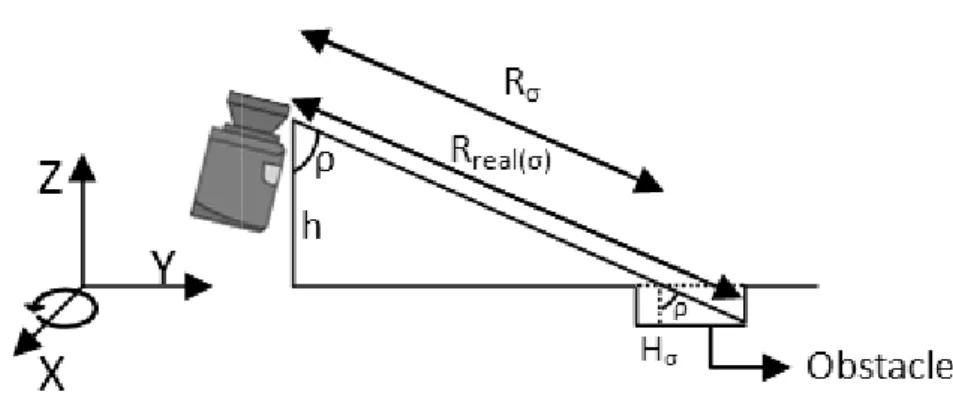
Figure 4.5 - Side view of the height computing process. Example for an obstacle placed on the positive Z axis. Hσ is the height in meters and ρ is an angle in degrees. ... 29

Figure 4.6 - Side view of the height computing process. Example for an obstacle placed on the negative Z axis. Hσ is the height in meters and ρ is an angle in degrees. ... 30

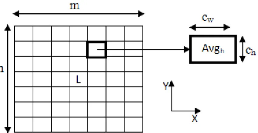
Figure 4.7 - Elevation map representation. n represents the number of height cells and m is the number of width cells. cw and ch represent cell’s width and height, respectively, measured in meters. L symbolizes LADAR’s position on the map. ... 31

Figure 4.8 - Obstacle map. nobs represents the number of height cells and mobs is the number of width cells. Cwobs and Chobs represent cell’s width and height, respectively, measured in meters. L symbolizes LADAR’s position on the map. cv represents each cell’s value. ... 32

Figure 4.9 - Flowchart of the mapping and obstacle detection system. ... 34

Figure 4.10 – Effects on the reference plane caused by variations on robot’s attitude. (a) and (b) - side view of pitch changes. (c) and (d) – front view of roll changes. (e) and (f) – top view of yaw changes. ... 35

Figure 4.11 – Computation of each XY point of the reference plane. (a) – side view, (b) top view. ... 36

Figure 4.12 – Example of point transformation. ... 39

Figure 4.13 - Implementation of this system on Player Server ... 41

Figure 4.14 – Run-time process of ladarDriv driver. ... 42

xx Figure 5.1 – The robot with which these experiments were performed. This robot is being developed by Holos, S.A., the mapping and obstacle detection system being the work of the author. ... 45 Figure 5.2 – Elevation and obstacle maps with different sizes and resolutions, all built in the same hall. (a) – real image of the hall. (b) and (c) – elevation and obstacle maps with 401x401 cells and resolution of 0.05 m. (d) and (e) – elevation and obstacle maps with 201x201 cells and resolution of 0.1 m. (f) and (g) – elevation and obstacle maps with 101x101 cells and resolution of 0.2 m. (h) and (i) – elevation and obstacle maps with 41x41 cells and resolution of 0.5 m. ... 49 Figure 5.3 – Reference plane experiment. (a) and (b) – real scene. (c) – elevation map. (d) – obstacle map. ... 51 Figure 5.4 – Experiment in which the robot goes down a ramp. (a) – real scene representing the ramp. (b) and (c) – elevation and obstacle maps taken before the robot start to go down the ramp. (d) and (e) - elevation and obstacle maps taken when the robot was already going down the ramp... 53 Figure 5.5 – Scrolling Procedure, first experiment. Beginning of the path: (a) – real scene, (b) – elevation map, (c) – obstacle map. End of the path: (d) – real scene, (e) - elevation map, (f) – obstacle map. ... 55 Figure 5.6 – Scrolling procedure, second experiment. Beginning of the path: (a) – real scene, (b) – elevation map, (c) – obstacle map. End of the path: (d) – real scene, (e) - elevation map, (f) – obstacle map. ... 57 Figure 5.7 - Corridor where this experiment was performed. (a) is the real scene, (b) the elevation map and (c) the obstacle map. ... 59 Figure 5.8 - Negative Pitch example. (a) – robot with negative pitch. (b) and (c) - elevation and obstacle maps with Pitch-Roll compensation. (d) and (e) - elevation and obstacle maps without Pitch-Roll compensation. ... 60 Figure 5.9 – Positive Pitch example. (a) – robot with positive pitch. (b) and (c) - elevation and obstacle maps with Pitch-Roll compensation. (d) and (e) - elevation and obstacle maps

without Pitch-Roll compensation. ... 62 Figure 5.10 - Negative Roll example. (a) – robot with negative roll. (b) and (c) - elevation and obstacle maps with Pitch-Roll compensation. (d) and (e) - elevation and obstacle maps

1

1.

Introduction

Nowadays, robots perform important roles in our society. They are present on many different areas such as automotive industry, entertainment, military operations, among others. In particular, mobile service robots employment has been widespread in the last years and today these kind of robots can perform several tasks like, for example, guiding tourists in museums [Chella et al., 2007], house cleaning, elderly care [Graf et al., 2004], interplanetary exploration [Cheng et al., 2005], or humanitarian demining [Santana et al., 2007].

The International Federation of Robotics (IFR) defines a service robot as “(…) a robot which operates semi- or fully autonomously to perform services useful to the well-being of humans and equipment, excluding manufacturing operations” [IFR, 2009]. Through this definition one can notice that autonomy is a key feature for a service robot. Therefore, and mostly on mobile service robots area, mapping is generally considered as one of the most important topics [Thrun, 2003]. In fact, once exploring an unknown area, the mobile service robot needs a process to construct a representation of the environment (map) and this can be used for navigation tasks such as path planning or obstacle detection and avoidance. Despite the fact that obstacle detection is often performed without using maps, it is also common to find approaches where mapping and obstacle detection are interconnected, which is the case in this dissertation. In this thesis, mapping is performed with the purpose to detect obstacles, i.e. obstacle detection will be accomplished with basis on the construction of terrain maps.

In order to build a map, a robot must be equipped with sensors that enable it to perceive its surroundings such as LADARs, Stereoscopic Cameras or Ultrasonic Range Sensors. Also, there are additional sensors that are often used in mapping including Inertial Measurement Units (IMU), Attitude and Heading Reference Systems (AHRS) or Global Positioning Systems (GPS).

2 LADARs and Stereoscopic Cameras are complementary and are often used simultaneously [Moghadam et al., 2008], [Matthies et al., 2002] and they both have advantages and disadvantages. A LADAR generally provides fast and accurate range measurements and works with big fields of view and at long ranges. However, it only provides information along the plane of the scanning laser beam and its performance is affected by weather conditions (such as fog or rain) and by objects reflectivity. On the other hand, Stereoscopic Cameras can provide 3D data and also color and texture information. Nevertheless, it generates large amounts of data (including noisy data) comparing to a LADAR, which can be computationally expensive to process and its measurements are affected by lightning conditions and by non-textured environments.

As mentioned before, the fusion of these two types of sensors is a common attempt to overcome their disadvantages and to take part of their main capabilities in order to build precise and reliable maps. However, in the context of this work a LADAR will be used as the only sensor for environment perception, mainly due to its accuracy and lower amount of generated data comparing to stereo vision. Also, the fusion of two or more range sensors will not be focused in the context of this thesis and, therefore, integration of stereo vision cameras and LADARs is discarded.

In the 1980s and early 1990s, two approaches for mapping were used: metric and topological [Thrun, 2003]. Metric maps can represent geometric features of the environment and two examples of this kind of maps are occupancy grid maps [Elfes, 1987] and feature maps [Chatila and Laumond, 1985]. In the former case, environments are represented by an occupancy grid where each cell can indicate the presence of an obstacle and in the latter case maps contain parametric features such as lines or arcs that intend to describe the environment. Topological maps can represent environments through connectivity between different places and an early example of this approach is the work of Kluipers and Byun [Kuipers and Byun, 1991]. In this case, the map contains a set of significant places that can be connected by arcs. These arcs are usually labeled with information about navigation from one place to another.

3 Over the last decades, several approaches have been proposed on the research field of obstacle detection systems for service robots. Some of the most successful ones are based on assumptions about terrain’s geometry [Konolige et al., 2008], [Batavia and Singh, 2002], on performing traversability analysis of the robot’s surroundings [Hamner et al., 2008], on creating representations of the environment and using them to detect obstacles or safe paths for the robot [Lacaze et al., 2002], on using statistical analysis of a 3D point cloud in order to characterize obstacles [Lalonde et al., 2006], or on describing obstacles in terms of geometrical relationships between 3D points [Manduchi et al., 2005]. These approaches are reviewed with more detail on chapter two.

The main goal of this dissertation is to present a LADAR-based solution for mapping and obstacle detection in structured environments, either indoor or outdoor. Off-road terrains are often unstructured environments and, consequently, they are beyond the scope of this work. In the context of this work it is assumed that the mapping and obstacle detection system travels in an unknown environment, i.e. the use of any a priori knowledge about its surroundings is discarded.

1.1

Problem Statement

As previously stated, this dissertation intends to present a solution for the problem of mapping and obstacle detection in indoor/outdoor structured environments that is targeted to a service robot equipped with a LADAR. In the development of such a solution, some main problems must be taken into consideration:

1. The proposed model must be suitable for structured environments (indoor or outdoor),

where structured surfaces must be correctly mapped and classified either as obstacles or freespace. As previously referred, off-road terrains are not considered in the context of this dissertation. Thus, unstructured surfaces may not be correctly mapped or classified.

4 3. The proposed model must be computationally efficient and cope with real-time

constraints, so that service robot’s safety can be assured.

1.2

Solution Prospect

In order to overcome the problems mentioned on the previous section, this dissertation proposes the following solutions:

1. In this model, obstacles are defined as surfaces that stand above or below the plane where the service robot is based and that can prevent a wheeled service robot from passing through. The LADAR is positioned in order to enable the system to detect obstacles that stand below LADAR’s height and also negative obstacles (obstacles that stand below the plane where the service robot is based), which are common in these environments.

2. The robustness in terms of variations on robot’s attitude is achieved with the help of an Attitude and Heading Reference System (AHRS) that provides pitch, roll and yaw

angles. This information is added to the mapping and obstacle detection algorithm so that it can be adapted to the current attitude values.

3. Although this model is based on the construction of terrain maps, which can require considerable storage capabilities, efforts were made to maintain low complexity on the algorithm and low computational cost on the performance of the system, mainly in the choice of an appropriate size and resolution for the maps.

This system is implemented on a framework for mobile robotics applications named

5

1.3

Dissertation Outline

This dissertation is organized as follows:

Chapter 1: introduces the reader to the subject of mapping and obstacle detection using a LADAR and lists some problems related to this subject. A solution prospect for these problems is also presented;

Chapter 2: exposes a brief overview of the state of the art about obstacle detection for service robots;

Chapter 3: gives an introduction to some supporting concepts used in this work;

Chapter 4: describes the mapping and obstacle detection system proposed;

Chapter 5: presents the experimental results;

7

2.

State of the Art

In the last decades, there have been a large number of contributions on the research field of obstacle detection systems for service robots. This chapter presents an overview of some approaches that were proposed on this area. In the sections of this chapter, the author’s intention is to present different approaches to the problem of obstacle detection for service robots, and not a historical evolution of the research in this area.

On section 2.1 an approach that uses the flat terrain assumption is presented. This method takes advantage of simplifications in order to simplify and speed up the process of detecting obstacles. Section 2.2 presents a method that was designed for terrains that show smooth slope changes and that uses gradient techniques to detect obstacles. A different approach is exposed on section 2.3. It uses traversability analysis of the robot’s surroundings instead of taking considerations about terrain’s geometry. Section 2.4 exhibits a method that creates a representation of the environment and uses it to detect safe paths for the robot. Section 2.5 shows an obstacle detection algorithm that performs statistical analysis of a 3D point cloud in order to characterize obstacles. Finally, a technique that describes obstacles in terms of geometrical relationships between 3D points is exhibited on section 2.6.

2.1

Flat terrain assumption

When travelling in outdoor conditions, an autonomous mobile robot may be confronted with structured environments such as urban terrains or man-made facilities, or with rougher terrains with great slope variations like the off-road case. Despite that, it is often possible to find a dominant ground plane. The presence of a ground plane simplifies processing and reduces the complexity of obstacles characterization. In fact, if a relatively flat ground plane is assumed, it is possible to simply define obstacles as salient surfaces standing above or below the ground.

8 point cloud of the environment and then the ground plane is determined by a RANSAC technique [Fischler and Bolles, 1981]. In this model, obstacles are defined as points that lie too high above the ground plane, but lower than the robot’s height. Sight lines are used to infer freespace to more distant points and their computation is achieved by finding columns of ground plane pixels that lead up to a distant obstacle. The color image is applied in path analysis. This work is illustrated in Figure 2.1.

Figure 2.1 - Visual processing diagram proposed by [Konolige et al., 2008].

This approach presents good results on flat terrains but, at the same time, is very susceptible to fail on rough ones where the determination of the dominant ground plane, which is the key feature of this kind of methods, is not very reliable. Besides that, the authors only consider obstacles as points that stand above the ground plane not taking into consideration “negative obstacles”, i.e. obstacles that stand below the ground plane, and this is a great drawback in outdoor navigation.

2.2

Obstacle detection in terrains with slightly variable

slope

In the previous section, obstacle detection was performed on the assumption of a flat terrain. In this section a more generic method that also deals with non-flat terrains is presented.

9 where the terrain changes his slope smoothly enough to define obstacles as discrete discontinuities.

The two-axis laser scanner used by the authors consists of a single line laser range finder that operates as a two-axis scanner by being rotated so that the laser scans vertically instead of horizontally, and then mechanically swept from side to side to provide horizontal coverage. In their work, the authors consider a “scan” as one line of laser data, scanned vertically, and a “sweep” as a set of scans, collected by mechanically sweeping the laser from side to side.

Figure 2.2 - Overview of the obstacle detection algorithm proposed by [Batavia and Singh, 2002]

The obstacle detection algorithm is summarized in Figure 2.2 and consists of two phases: classification and fusion. In the classification phase, each scan line is converted to Cartesian coordinates and terrain’s gradient is computed along the scan line. A threshold is then applied to the gradient to classify each pixel as ‘obstacle’ (dark dots on Figure 2.2) or ‘freespace’ (white dots on Figure 2.2). Each classified scan is then saved in a buffer containing a time-history of scans. This buffer is represented on the block named “Cartesian View” on Figure 2.2. The duration of this ‘time window’ establishes the amount of data that will be fused. In the fusion phase, obstacle pixels are clustered using a nearest neighbor (NN) criterion and candidate obstacles are then filtered based on their mass and size.

10

2.3

Traversability

Rather than taking geometric considerations about the terrain, there are some approaches that employ traversability analysis. Instead of determining if a certain region of the environment is an obstacle or freespace, this kind of obstacle detection systems try to avoid such a binary decision assigning to each region of the robot surroundings a cost value that represents the degree of difficulty for the robot to move across that region.

Hamner et al. [Hamner et al., 2008] present an obstacle detection system that performs traversability analysis. The authors use two laser range finders (one that is fixed and another that sweeps about an orthogonal axis) and a sliding window of point cloud data (obtained from both lasers) that is registered over time. Vehicle-sized planar patches are fit to the point cloud data and this process allows the settlement of three parameters: plane orientation (roll, pitch), terrain’s roughness (obtained by the residual of the fitting process) and the height of data points above the plane. This method produces a grid-based traversability map and the plane fitting process is applied to each cell of the map, in order to acquire the parameters that are used to compute a hazard score that corresponds to the traversability measure of each cell. Furthermore, the authors complement the traversability analysis with gradient analysis from [Batavia and Singh, 2002] presented in section 2.2 in order to improve their results.

The plane fitting process performed in this work has a large computational cost and this is a main concern in real-time obstacle detection for mobile robots. Although it compensates some weaknesses of each individual algorithm, the option of combining two different kinds of analysis for obstacle detection increases the complexity of the system. This system is also more expensive than other approaches because it makes use of two laser scanners and a sweeping system.

2.4

Representations of the environment

Lacaze et al. [Lacaze e in order to detect the sup measurements of a LADAR the vehicle and this is done tile of the map is assigned threshold is applied to the Then, the authors try to p through the computation of depend on several parame terrain, number of times ea trajectory. The authors use placing vehicle masks along

Instead of assessing th elevation map to estimate makes the method comput vehicle masks, and causes it

2.5

Statistical an

Lalonde et al. [Lalond detection. In this work the point cloud that is built incr

Figure 2.3 - The three c

e et al., 2002] propose the creation of an elevat upport surface for the vehicle and to avoid AR are geometrically transformed into an eleva ne as the vehicle moves through the terrain. Du

d with the number of times it has been seen by he elevation map to determine the support su

predict safe trajectories for the vehicle alon of cost functions for each potential trajectory meters such as existence of protruding objec each cell has been seen by the sensor and pitc

use a vehicle model to predict pitch and roll ng each potential trajectory in the elevation ma

the content of each tile to try to find obstacle te safe trajectories for the robot by calculating

putationally heavy, especially because of the s it to have difficulties to deal with real-time co

analysis

nde et al., 2006] propose a different technique e authors present a method that employs statis crementally as the robot navigates through the

e classes used by [Lalonde et al., 2006] to classify th

11 ation map of the terrain id obstacles. First, the evation map centered on During this process each by the sensor. A height surface for the vehicle. long the elevation map ry. These cost functions jects, roughness of the itch and roll along each roll along each path by map.

cles, the authors use the ing cost functions. This the multiple placing of constraints.

que to perform obstacle tistical analysis of a 3D he terrain.

12 This analysis tries to classify the 3D point cloud into three classes: surfaces (ground surface, rocks), linear structures (wires, branches) and scattered regions (vegetation). The classification is based on the comparison of the eigenvalues obtained from the calculation of a covariance matrix for all the points within a neighborhood of a certain point.

As shown on Figure 2.3, scattered regions have no dominant eigenvalue whereas linear structures present one main eigenvalue and surfaces have two eigenvalues that prevail.

This obstacle detection algorithm is suitable for vegetated terrains and the authors present good results using measurements from laser scanners but, nonetheless, for structured environments simpler approaches can be used.

2.6

Geometrical relationships

A method that examines geometrical relationships between points of a 3D point cloud was developed by Manduchi et al. [Manduchi et al., 2005]. These authors try to detect obstacles by analyzing slant and altitude of visible surface patches directly in the range image domain. A visible surface patch is considered an obstacle if its slope is larger than a certain value θ (the maximum slope a robot can climb) and if it spans a vertical interval larger than a threshold H (the minimum height an obstacle must have to block robot’s passage). Slant and altitude measures are taken from the search for pairs of compatible points in the 3D point cloud.

13 This compatibility relationship is illustrated in Figure 2.4 and is expressed by the authors as follows: “The points compatible with a surface point p are those belonging to the two truncated cones Up and Lp with vertex in p, axis oriented vertically, and limited by the two planes of equation y = Hmin and y = Hmax respectively ” [Manduchi et al., 2005].

Each point is considered an obstacle point if it has at least one compatible point that belongs to the same surface. The authors use stereo-vision images and, for each image pixel, a search for compatible points is executed with the aim of finding obstacle points.

15

3.

Supporting concepts

This chapter summarizes some concepts that helped on the development of this mapping and obstacle detection system. Section 3.1 describes some coordinate systems and coordinate transformations that are useful in mobile robotics. Section 3.2 presents the Player/Stage Project, which is an open-source framework that simplifies the development of control architectures for several applications, including mobile robots.

3.1

Coordinate Systems and Coordinate Transformations

There are many ways of representing a location in the world by a set of coordinates. This section presents some coordinate systems that are often used in navigation with Inertial Navigation Systems [Grewal et al., 2001]. Coordinate transformations that are useful in mobile robotics and, in particular, in this work, are also exposed in this section.

3.1.1 LTP coordinates

Grewal defines Local Tangent Plane (LTP) coordinates as “(…) local reference

directions for representing vehicle attitude and velocity for operation on or near the surface of the earth” [Grewal et al., 2001]. A frequent orientation for this kind of coordinates has one horizontal axis (the east axis) in the direction of increasing longitude and the other horizontal axis (the north axis) in the direction of increasing latitude. A common LTP coordinate system is the North-East-Down (NED).

In NED, the direction of a clockwise turn is in the positive direction with respect to a downward axis. This coordinate system is used in many applications because its coordinate axes coincide with vehicle-fixed roll-pitch-yaw (RPY) coordinates when the vehicle is level and headed north [Grewal et al., 2001].

3.1.2 RPY coordinates

Grewal [Grewal et al., 2001] defines roll-pitch-yaw (RPY) coordinates as “(…)

16

right-hand side, and the yaw axis such that turning to the right is positive”. Figure 3.1 illustrates this coordinate system.

Figure 3.1 – Roll, Pitch and Yaw axes [Grewal et al., 2001].

The angles of rotation about the vehicle roll, pitch and yaw axes are called the Euler

angles [Grewal et al., 2001]. These angles can specify the attitude of the vehicle body with respect to local coordinates.

Figure 3.2 – Vehicle Euler Angles defined by Grewal [Grewal et al., 2001].

A common convention for Euler angles is illustrated on Figure 3.2 and is defined by Grewal [Grewal et al., 2001] as a set of three rotations, starting with the vehicle level with roll

• First rotate thro azimuth (headin (east) from nort

• Then, rotate thr

vehicle roll axis from the local h

• Finally, rotate t vehicle attitude

Figure 3.3 illustrates ho an object, in this case an air

Figure 3.3 – Ro

This set of three angul bring one coordinate frame specified by a rotation m coordinates to NED coordin on Figure 3.4 [Grewal et al.

rough the yaw angle (Y) about the vehicle yaw

ding) of the vehicle roll axis. The azimuth is orth;

through the pitch angle (P) about the vehicle p

xis to its intended elevation. Elevation is meas l horizontal plane;

e through the roll angle (R) about the vehicle de to the specified orientation.

how the rotations through these angles can af airplane.

Rotations through Roll, Pitch and Yaw angles [ACME

ular rotations is often used to define a coordin e to coincide to another. To achieve this, the r matrix. For example, the coordinate transf rdinates is given by the product of three rotatio al., 2001].

17

yaw axis to the intended is measured clockwise

pitch axis to bring the easured positive upward

le roll axis to bring the

affect the orientation of

ME, 2009].

18

Figure 3.4 - Transformation from RPY coordinates to NED coordinates [Grewal et al., 2001].

A similar convention for Euler angles is given by Craig [Craig, 2005]. Given two frames

A and B, the order of rotations is as follows: starting with frame B coincident with a known frame A, rotate first B about ZB by an angle α, then about YB by an angle ß, and, finally, about

XB by an angle γ. This set of Euler-angle rotations is exemplified on Figure 3.5.

Figure 3.5 - Euler Angles defined by Craig [Craig, 2005].

The final orientation of B relative to A is also given by the product of three rotation matrices, as follows:

R , , α, β, γ = R α R β R γ

= cos α − sin α 0sin α cos α 0

0 0 1) ∙

cos β 0 sin β

0 1 0

−sin β 0 cos β) ∙

1 0 0

0 cos γ −sin γ

19 = cos α cos β − sin α cos γ + cos α sin β sin γsin α cos β cos α cos γ + sin α sin β sin γ − cos α sin γ + sin α sin β cos γsin α sin γ + cos α sin β cos γ

− sin β cos β sin γ cos β cos γ )

Equation 3.1

If one considers that the Euler angles of Craig’s [Craig, 2005] convention, α, ß and γ, correspond, respectively, to the Euler angles of Grewal’s [Grewal et al., 2001] convention, Y,

P and R, one can see that the results from Figure 3.4 and from Equation 3.1 are equivalent.

3.2

Player/Stage Project

The Player/Stage Project provides open-source tools that simplify controller development, particularly for multiple-robot, distributed robot, and sensor network systems [Vaughan et al., 2003]. This project includes the Player server, and the robot simulators Stage

and Gazebo. According to its authors and developers, the Player server “(…) is probably the most widely used robot control interface in the world.” [Player Project, 2010].

Player is a network server for robot control [Player Project Wiki, 2010]. When operating on a robot, Player provides a straightforward interface to the robot’s actuators and sensors over an IP network. The user can create a Client program that configures devices, reads data from sensors and writes commands to actuators by interacting with Player over a TCP socket.

Stage is a 2D multiple-robot simulator from the Player project [Player Project Wiki, 2010]. It can simulate a group of mobile robots driving and sensing a two-dimensional environment. This simulator is prepared to provide virtual robots that make use of simulated devices instead of physical sensors, taking advantage of several sensor models including sonars, laser rangefinders, cameras, etc.

Gazebo is a multi-robot simulator for outdoor environments [Player Project Wiki, 2010]. Its basis is similar to Stage, but the robots and sensors are simulated on a three-dimensional environment.

Player server is the only component of the Player/Stage Project that will be used in this work and, thus, it’s also the only one of the three components that is explored in more detail in this chapter.

Player defines a set of standard interfaces, each of which is a specification of the ways that you can interact with some class of devices [Player Manual, 2010]. For example, the

20 can return its measurements (generally, a list of ranges and some scanning parameters). This

interface can be used to interact with different kinds of laser range finders, such as SICK and Hokuyo Laser Range Finders.

Another key concept in Player is the concept of driver. It is defined by the authors of Player Project as “A piece of software (usually written in C++) that talks to a robotic sensor, actuator, or algorithm, and translates its inputs and outputs to conform to one or more interfaces” [Player Manual, 2010]. The driver’s job is to adapt the specific language of an equipment or algorithm to the format of the corresponding interface. This way, two different sensors of the same class can provide data in the same format to Player, using the same interface. Most Player drivers communicate directly with hardware, but it’s also possible to use a different kind of driver - the abstract driver - that communicates with other drivers instead of hardware components. Player has a lot of drivers and abstract drivers already developed and that are ready to be used by the developer.

The concept of device is closely linked with the concepts above mentioned. A device

represents a connection between a driver (or an abstract driver) and an interface. Each device

is assigned with a specific address that is used for message exchange which occurs between

devices and with the help of interfaces [Player Manual, 2010]. This address can be composed by several fields such as host, robot (port), interface or index. Only the last two fields are mandatory [Owen, 2010].

The connection between a driver and an interface is specified in a configuration file, named config file. The user must write this file containing all the information that Player must know about the equipment that will be used. This file tells Player which drivers will be used and which interfaces they provide or require. The declarations of drivers or abstract drivers

on the config file can also contain some parameters related to the sensor or algorithm that corresponds to the driver or abstract driver, respectively.

The relationships between these three important concepts of Player (interface, driver and

device) can be easily understood with the help of an example: As mentioned before, there are several drivers that came with Player. One of them is the sicklms200 driver. This driver

controls a SICK LMS200, which is a laser range finder that is popular in mobile robotics applications. This driver is able to communicate with the SICK LMS200 over a serial port and receive range data from it. Moreover, the sicklms200 driver translates the range data received in a specific SICK format to the format defined by the laser interface. Thus, Player

must know that this driver provides a laser interface. To achieve this, the sicklms200driver

21 On this example, a driver with the name sicklms200 is declared. The device address is defined on the ‘provides’ section. This address is composed by the laser interface (the

interface through which the driver provides data) and the index of the device which is 0. It also has a parameter named scanning frequency with the value 50.

The Player/Stage Project has also a set of libraries, named Client Libraries, which allow

the user to communicate with the Player server from an external program. This

communication can be achieved by using Proxies that are defined in the Client Libraries.

Proxies are C++ classes that offer methods to request data and/or send commands from and to the Player server and they are closely related to the interfaces defined on Player, i.e. for each

interface there should be a corresponding Proxy in the Client Libraries. The user must build a

Client program that uses Proxies to communicate with Player, in order to request data from sensors and send commands to actuators.

The global architecture of the Player/Stage Project is illustrated on Figure 3.6.

Figure 3.6 - Global architecture of Player/Stage Project

driver

(

name "sicklms200" // name of the driver

provides ["laser:0"] // [“interface:index”]

scanning frequency 50 // parameter

22 This figure shows that the Client program built by the user requests data or sends

commands through the methods contained in Proxies. These methods offered by Proxies are

prepared to send messages to drivers in order to deliver those requests and/or commands. These messages are routed by Player Server that knows which interfaces each driver supports and which Proxies correspond to those interfaces. Finally, the drivers communicate with the hardware of the robot to perform the actions desired by the Client.

As referred before, Player has several drivers and abstract drivers already developed. However, the user may not have the hardware or may not want the algorithms that these

drivers control. In these situations, the user should develop its own driver. For this, it’s

important to know the methods contained on a driver and its run-time process. The methods

that should be present on a driver are:

• Driver(ConfigFile* cf) : The constructor of the driver. It reads all the information present on the config file that is related to this driver, including the

interfaces it provides and/or requires and some parameters that may have been defined. The parameter cf represents the config file that loads the driver;

• MainSetup() : This method allocates resources before entering the main loop. It is also useful to perform initializations or error checking before the main loop becomes active. In general, the developer should put here everything that only needs to be done once;

• pthread_testcancel() : This function is prepared to check whether the driver’s thread should be killed and to cause the driver to break out of the Main() loop

and go to the MainShutdown() method;

• ProcessMessages() : A very important method that processes the messages present on the message queue. In this method, the driver can receive data (e.g. from other drivers) and requests (e.g. from Clients). The driver can publish its data here, if it receives requests for it;

23

ProcessMessages() or pthread_testcancel(). If the driver doesn’t need a request to publish its data, it can be published in the Main function;

• MainShutdown() : This method is called when the driver is about to be stopped by Player. It’s useful to deallocate resources, disconnect from ports, etc;

• ~Driver () : The destructor of the driver.

The run-time process of a Player driver is exemplified on Figure 3.7 [PSU Robotics RoboWiki, 2010].

Figure 3.7 - Run-time process of a Player driver [PSU Robotics RoboWiki, 2010].

First, the Constructor and the MainSetup methods are executed. Then, the driver enters in its core function, i.e. the Main loop. In this loop, the driver continuously verifies if Player

wants it to be stopped and also checks for new messages, executes the corresponding actions and publishes new data. Finally, when the driver is stopped, the MainShutdown and the

25

4.

Mapping and Obstacle Detection system

This chapter presents a mapping and obstacle detection system for service robots that work in indoor/outdoor structured environments and that are equipped with, mainly, a LADAR and an AHRS sensor. Section 4.1 shows how the LADAR is positioned in this system, in order to build elevation maps of the environment. Section 4.2 exposes the mapping procedure that is responsible for the creation of the elevation map. On Section 4.3, it is described the obstacle definition used in this model. This definition and the previously obtained elevation maps are used by a simple obstacle detector, which is described on Section 4.4. This obstacle detection procedure generates a map (obstacle map) that represents only obstacles and freespace and that is more suitable to be used by a path planner than an

elevation map. Section 4.5 presents the scrolling procedure that is used for the elevation map

and depicts the overall functioning of this mapping and obstacle detection system. Section 4.6 describes the attitude compensation procedure used on this system. This algorithm uses an AHRS sensor and allows this system to be more robust against variations on robot’s pitch,

roll and yaw angles. Finally, Section 4.7 describes the implementation of this mapping and obstacle detection system on a platform for robotic applications named Player/Stage.

4.1

LADAR’s positioning

Figure 4.1 – LADAR features. d1 and

Typically, the LADAR can b of the environment. The 2D app parallel to the floor. If we consi obtained with this method is show

(a)

Figure 4.2 – Two types of maps obtain

This kind of maps is acceptab have specific shapes and shoul However, this method faces many or above the height of the LADA dissertation the LADAR is used

nd dn are measured distances, α is the angular step an

view.

n be used to build two dimensional or three dim approach is normally achieved by setting the nsider the hallway presented in Figure 4.2 (a)

own in Figure 4.2 (b).

(b)

tained using a LADAR. (a): Hallway; (b): 2D map of of (a).

table for a two dimensional world where all the uld be tall enough to be detected by the s any problems presented by the real world such a AR, tables, sidewalks, fencings, ditches, amon ed in a way suitable for a three dimensional w

26

and θ is the field of

dimensional maps he scanning plane (a), a typical map

(c)

of (a); (c): 2.5D map

the objects should e scanning plane.

approach it is possible to bu on Figure 4.2 (c).

As stated before, this robot, with the scanning p Figure 4.3. As the robot mo a 2D ½ map is being built.

Fig

4.2

Mapping

This section exposes th describes the computation information that will be add 4.2.2).

4.2.1 Computation o

One of the first operat

plane, which is the plane th any object inside its field of ranges that the LADAR wo and no other object or su

build two and a half dimensional maps, simila

is model uses a single LADAR which is place plane angled down towards the direction of moves forward, the laser sweeps some space in

Figure 4.3 – LADAR’s positioning for this model.

the procedure that is behind the creation of on of the reference plane (section 4.2.1) and dded to the elevation map and how the map i

n of the reference plane

rations of the mapping procedure is the compu that the LADAR “sees”, positioned as on Figu

of view. In other words, it’s an “empty plane” would provide if it only scans the surface where

surface is detected in its field of view. Th

27 ilar to the one presented

aced on top of a mobile of motion, as shown in in front of the robot and

of the elevation map. It nd also how to get the is represented (section

putation of a reference

continuously updated due to chan

real plane4 provided by the LADA The calculation of the refere

which are illustrated on Figure 4. is on the position (0, 0, h) acco represents the theoretical range p emitted at , =90°. LADAR’s h LADAR’s tilt (ϕ = 90◦ - tilt).

(a)

Figure 4.4 – Calculatio

On Figure 4.4 (a) it’s possib equation:

LADAR’s height and tilt rem in a fix position. Thus, it would b long as h and ϕ remain constant because d will have to be updated explored on section 4.5.

Then, distance d is used to c as follows:

4

In this dissertation, the term "real plane LADAR at each scan.

hanges in LADAR’s attitude and is used to co DAR in order to obtain information about terra

erence plane is based on some simple trigono .4. In these calculations it is assumed that the cording to the coordinate systems of Figure

provided by the LADAR’s central beam, i.e. s height is represented by h and ϕ is an angle

(b)

tion of the reference plane: (a) side view, (b) front vie

sible to see that distance d can be computed b

/ _{cos 1}0

remain always with the same value, since the L d be expected that distance d would always rem nt and no obstacles are detected. In fact, this ted due to changes in robot’s attitude, but this

compute the LADAR’s theoretical range at ea

lane" refers to the plane that contains the set of ranges m

28 compare with the rrain’s elevation.

nometry concepts, the LADAR’s lens re 4.4. Distance d

e. the beam that is gle obtained from

view.

d by the following

e LADAR is fixed emain the same as is will not happen is problem will be

t each angle σ (Rσ)

The angle σ represents obtained by iteratively addi field of view.

The reference plane wi view of the LADAR. Summ first computing distance d

angle σ of the field of view.

4.2.2 Map building

As stated before, the elevation by comparing it w scan is performed, and for compared to the correspon hypothetical obstacle. This p

Figure 4.5 - Side view of the h axis. H

By looking at Figure 4 can be computed by the foll

2 _{sin ,}/

nts each angle where the LADAR emits a be dding the angular step α (see Figure 4.1) to the

will be composed by the set of Rσ ranges compu mmarizing, the procedure to compute the refere d and then using this distance to determine t w.

he reference plane is used to obtain inform

it with the real plane provided by the LADAR

or each angle σ, the real range provided by th onding range Rσ of the reference plane to com is procedure is illustrated on Figure 4.5 and Fig

e height computing process. Example for an obstacle

Hσ is the height in meters and ρ is an angle in degree

4.5 it’s possible to see that the height of a hypo ollowing equation:

3 cos 4 5 62 $ 2 78 9

29 beam. These angles are the starting angle of the

puted along the field of

ference plane consists of e the range Rσ for each

rmation about terrain’s R. Hence, every time a the LADAR (Rreal(σ)) is

compute the height of a igure 4.6.

placed on the positive Z es.

The angle ρ is obtained

For “negative” obstacles, i.e similar but, in this case, Rreal(σ) h

expected, the value obtained to H

Figure 4.6 - Side view of the height c axis. Hσ is the

If there isn’t any obstacle at same value and the value compute

Finally, the computed heig representation of the terrain’s ele LADAR. A grid map was adop Figure 4.7). This map can be repre

The elevation map is a two based on the measures taken from placed on the center cell of the m Each cell in the elevation map re

ed from laser’s height h and each range Rσ as fo

4 cos:;_<0 2 =

i.e. obstacles placed on the negative Z axis, has a bigger value than Rσ, as shown on Figur

Hσ is negative.

t computing process. Example for an obstacle placed he height in meters and ρ is an angle in degrees.

at a given angle σ, Rreal(σ) and Rσ will have ap uted for 3 will be very close to zero.

ight (Hσ) is saved in an elevation map (sy elevation) on a cell corresponding to the range

opted to represent terrain’s elevation in a su presented by the following expression:

> > ?@AB CB ,D DE

DEF EG

EF

o-dimensional array of cells (H 5 contain rom the LADAR and it is LADAR-centered, i map, which is also considered as the origin o represents an area, I_B5 I_J m2. Therefore, t

30 follows:

the procedure is ure 4.6. Hence, as

ed on the negative Z

approximately the

(system’s internal ge provided by the suitable way (see

31 the map is H 5 I_J 5 5 I_B m2. Each cell contains the average of the heights of all computed points that correspond to that cell. A representation of the elevation map used in this work is shown on Figure 4.7.

Figure 4.7 - Elevation map representation. n represents the number of height cells and m is the number of width cells. cw and ch represent cell’s width and height, respectively, measured in meters. L symbolizes

LADAR’s position on the map.

Every time a LADAR scan is performed, the elevation map is updated with new information obtained from the scan. To achieve this, the average height of each cell that contains new information is updated with the corresponding height values computed from the new scan, as explained before.

4.3

Obstacle definition

As previously stated, this model intends to be suitable for structured environments. These environments usually have large planar surfaces where, generally, obstacles are distinguishable. Thus, in this case, an obstacle can be understood as an object that stands above or below those large planar surfaces where the service robot is based and that can prevent a wheeled service robot from passing through. In this model, it is assumed that the surface where the robot stands is considered as the ground plane and obstacles are classified in terms of their heights in relation to this ground plane. The obstacle definition used is:

32 1. M@A_B K, L > 3_OP ∪ M@A_B K, L < 3 _C

where M@A_B K, L is the average height of the cell, 3_OP is the minimum height that an object that stands above the ground plane must have to be considered as an obstacle and 3 _C is the minimum height that an object that stands below the ground plane must have to be considered as an obstacle. All the cells that have average heights with values between 3_OP and 3 _C are considered as free space. Consequently, the values for parameters 3_OP and 3 _C must be chosen according to the service robot’s dimensions in order to prevent the robot being damage when travelling cells considered as free space.

4.4

Obstacle detection

The obstacle detection procedure of this model is very simple and consists in applying the obstacle definition of section 4.3 to each cell of the elevation map. The information obtained on the obstacle detection procedure is saved on an obstacle map (see Figure 4.8) that is more suitable to be transferred to and used by a path planner.

The obstacle map is similar to the elevation map in terms of their appearance. Nonetheless, the content of each cell is different. In the obstacle map, each cell holds a value (cv) that represents an obstacle or free space.

Figure 4.8 - Obstacle map. nobsrepresents the number of height cells and mobs is the number of width cells. Cwobs and Chobs represent cell’s width and height, respectively, measured in meters. L symbolizes

33 Also their heights and widths can be different, because if the obstacle map is intended to be used by a path planner its size could be smaller than the elevation map’s size in order to reduce the amount of information that is transferred. For example, the obstacle map can represent only a “window” of the elevation map maintaining the same resolution (cell’s size). However, these details must be taken in consideration according to the chosen strategy for the path planning.

As previously mentioned, the value assigned to each cell of the obstacle map depends on the results of applying the obstacle detection definition to the elevation map. This value is assigned according to the following conditions:

IS T$1_{1, M@A}, 3 C < M@AB K, L < 3OP

B K, L > 3OP ∪ M@AB K, L < 3 CU

If a cell of the elevation map is considered an obstacle, the corresponding cell of the

obstacle map is assigned with the value 1. If the cell is considered as free space, the corresponding cell of the obstacle map is assigned with the value -1. This procedure is performed only for the cells of the elevation map that contain information in order to increase the computational efficiency of this procedure. The cells of the obstacle map that correspond to those of the elevation map that have no information are assigned with the value 0, which means “unknown terrain”.

4.5

Map scrolling

Before the calculation and addition of new information, there is the possibility of

elevation map’s cells being repositioned according to LADAR’s displacement, but only when this displacement is larger than a cell’s size. In this scrolling procedure, cells are only repositioned across the Y axis, i.e. each cell remains in the same column, changing only its line. Therefore, in order to decide if the scrolling procedure must be executed, the Y axis projection of LADAR’s displacement is computed (using yaw angle) and this value is the one that is compared with the cell’s size. Also, only the cells that contain information are repositioned, which increases the computational efficiency of this procedure.

Figure 4.9 - Flowchchart of the mapping and obstacle detection system.

34

First, and only if LAD

map is scrolled according

procedure for Yaw compens

updated according to the L 4.9 as Pitch-Roll compensat

is stored so it can be used t is performed. Afterwards, th obtain information about ter

map. Finally, the obstacle d as explained on section 4.4.

(a)

(c)

(e)

Figure 4.10 – Effects on the view of pitch changes. (c) an

DAR’s displacement is bigger than the size o ng to this displacement and Yaw compensatio ensation is addressed on section 4.6. After that,

LADAR’s pitch and roll angles. This procedu

sation is also explored on section 4.6. Then, the d the next time that this whole procedure, repre , the new reference plane and the real plane are terrain’s elevation and this new information is e detection procedure is performed in order to b

.4.

(b)

(d)

(f)

e reference plane caused by variations on robot’s atti and (d) – front view of roll changes. (e) and (f) – top

35 e of a cell, the elevation ation is performed. The at, the reference plane is edure, named on Figure the new reference plane

presented on Figure 4.9, are compared in order to is added to the elevation

build the obstacle map,