Automatic engine and propeller selection for mission and performance optimization

(1)

UNIVERSIDADE DA BEIRA INTERIOR

Engenharia Aeronáutica

Automatic engine and propeller selection for

mission and performance optimization

(versão corrigida após defesa)

Nídia Salvador Ribau

Dissertação para obtenção do Grau de Mestre em

Engenharia Aeronáutica

(ciclo de estudos integrado)

Orientador: Prof. Doutor Pedro Vieira Gamboa

(2)

(3)

(4)

(5)

Acknowledgements

Throughout the course of this dissertation I was blessed to have the help and support of a faithful amount of people, which gave me motivation and focus to finish and deliver an honest work to be proud of.

Without further delays, I would like to thank my advisor, Professor Pedro Vieira Gamboa, for his precise and utmost needed guidance, which enabled me to complete this thesis.

I would also like to thank from the bottom of my heart to my big little family, which always encouraged me to finish my studies and helped me financially in all matters. Without them I could not have completed this stage.

At last, I would like to thank all my dear and close friends which accompanied me through all these college years and with whom I had the pleasure to share astonishing moments.

(6)

(7)

Resumo

Nesta dissertação, um programa de otimização já existente foi empregue de modo a minimizar a energia consumida durante uma dada missão. Inicialmente, o algoritmo de otimização apenas devolve os valores otimizados das variáveis de projeto referentes à hélice, e nenhum constrangimento no desempenho da missão pode ser imposto. Assim sendo, dois principais objetivos são estipulados nesta tese. Primeiramente, permitir a otimização de variáveis de projeto referentes ao sistema propulsivo, de modo a efetuar a correspondência adequada com a hélice. Por conseguinte, é necessário criar duas bases de dados, uma com as especificações do motor elétrico e outra com as especificações do motor a combustão, de modo a desenvolver modelos empíricos dependentes the certas variáveis de projeto. Estas variáveis são então introduzidas no algoritmo de optimização, para que sejam otimizadas em conjunto com os parametros de projeto da hélice. O segundo objetivo estabelecido é adicionar certos constrangimentos relativos ao desempenho da missão, para possibilitar ao utilizador o constrangimento de certos parâmetros dentro de cada iteração do algoritmo.

Ambas as bases de dados foram criadas com sucesso, obtendo-se assim os modelos empíricos desejados, apesar de estes possuirem um determinado erro associado aos coeficientes das funções. As variáveis de projeto selecionadas para serem introduzidas no algoritmo foram a potência útil máxima e a velocidade do motor máxima no caso dos motores a combustão, e a corrente máxima e a constante de velocidade do motor no caso do motor eléctrico. Os constrangimentos da missão foram também calculados e introduzidos dentro do algoritmo, sendo que este otimiza de acordo com o espaço viável definido pelo utilizador.

O programa atualizado devolve, para um dado conjunto de constrangimentos relativos ao desempenho da missão, a solução do motor que corresponde às variáveis de projeto otimizadas da hélice, e seleciona um motor real a partir da base de dados criada. Os resultados obtidos confirmam que os modelos empiricos dos motores revelam-se bastante pragmáticos, possibilitanto boas correspondências para com a solução ótima, apesar de não serem perfeitas. As variáveis de projeto e a função objetivo convergem corretamente para uma solução estável, de acordo com o espaço viável que o utilizador pode optar por definir.

Palavras-chave

(8)

(9)

Abstract

In this dissertation, an already existing optimization software is employed to minimize the total energy consumed at a certain given mission. Initially, the optimization algorithm only returns the optimized design variables for the propeller specifications, and no mission performance constraints can be defined. Hence, on this thesis, two main objectives are stipulated. One is to enable the optimization of certain engine/motor design parameters to match the propeller. Thus it is required to create two data bases, one with the IC engine specifications and another with the electric motor specifications, in order to develop empirical models as functions of certain design variables. These engine design variables are then inputted into the optimization algorithm, to be optimized alongside the propeller parameters. The second objective established is to add certain mission performance constraints, to enable the user to constrain certain parameters inside the algorithm iterations.

Both data bases were successfully created, and all empirical models obtained, although with a certain error associated with the coefficients of the functions. The design variables selected to be introduced in the algorithm, which are the inputs of the empirical models, were rated power and rated engine speed for the IC engine, and maximum allowed current and the motor speed constant for the electric motor. The mission constrains are also calculated and inputted inside the algorithm, optimizing according to the feasible space defined by the user.

The updated software now returns, for a given set of mission constraints, the engine solution which matches the optimized propeller parameters, and selects a real engine from the database created. The results obtained confirmed the practicality of the engine empirical models, given good matches, although not perfect, to the optimum solution reached. The design variables and the objective function are converging correctly to a stabilized solution, according to the feasible space the user may choose to define.

Keywords

(10)

(11)

List of Figures

Figure 1.1 Optimization Process ... 5

Figure 1.2 Non-convex function [18] ... 8

Figure 1.3 2D representantion of the solution path of the steepest descent method [19] ... 9

Figure 1.4 2D representation of the solution path of the conjugate gradient method [19] ... 9

Figure 1.5 3D representation of 𝑓(𝑥1, 𝑥2) [19] ... 9

Figure 2.1 Relation between IC engine performance parameters ... 13

Figure 2.2 Energy Distribution in the IC Engine [22] ... 14

Figure 2.3 Torque, brake power and brake specific fuel consumption as a function of engine speed [26] ... 14

Figure 2.4 Brake specific fuel consumption as a function of engine throttle [27] ... 15

Figure 2.5 Approximated linear regression for 𝑏𝑝, at sea level and full load ... 16

Figure 2.6 Depiction of motor losses [29] ... 18

Figure 2.7 Relation between the electric motor performance parameters ... 18

Figure 2.8 Relation between motor torque and speed [30] ... 19

Figure 2.9 Relation between motor torque and current [30] ... 20

Figure 2.10 Relations between motor parameters to motor torque [31] ... 20

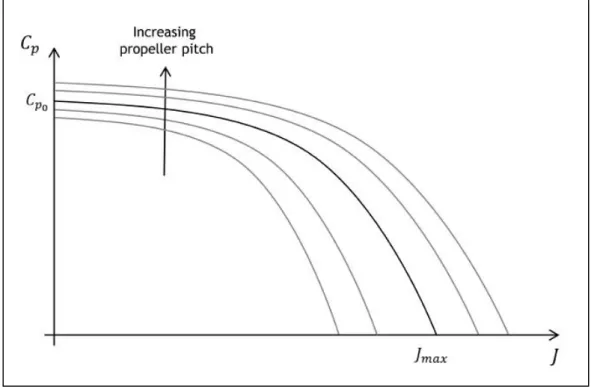
Figure 2.11 Propeller 𝐶𝑝(𝐷, 𝑝, 𝐽) for various pitch [27]... 26

Figure 2.12 Propeller 𝜂𝑝(𝐷, 𝑝, 𝐽) for various pitch [27] ... 27

Figure 2.13 Force diagram for steady, level flight [35] ... 28

Figure 2.14 Total drag versus air speed [35] ... 30

Figure 2.15 Effect of altitude on required power [34] ... 30

Figure 2.16 Effect of altitude on available thrust of a propeller driven aircraft [35] ... 30

Figure 2.17 Power available and power required as a function of air speed [37] ... 31

Figure 2.18 Force and speed diagram for climbing flight [35] ... 32

Figure 2.19 Rate of climb as a function of air speed [35] ... 33

Figure 2.20 Point of null excess of power available, at the service ceiling altitude [35] ... 34

Figure 2.21 Variation of maximum rate of climb with altitude [34] ... 34

Figure 2.22 Top view of a level turn [34]... 34

Figure 2.23 Balance of the acting forces on a level turn [34] ... 34

Figure 2.24 Flight envelope diagram [36] ... 36

Figure 2.25 Forces acting on the aircraft during takeoff performance [35] ... 38

Figure 2.26 Typical coefficient of friction for different ground surfaces [35] ... 38

Figure 2.27 Ground roll [35] ... 39

Figure 2.28 Relation between runway distance, altitude and weight [36] ... 42

Figure 3.1 Brief introduction of the overall optimization process ... 43

Figure 3.2 Simplified scheme of the forward finite differences method used to estimate the gradient at point 𝑥 ... 46

(16)

Figure 3.4 Typical specific fuel consumptions charts provided for Lycoming O-360 and HO-360

[46] ... 49

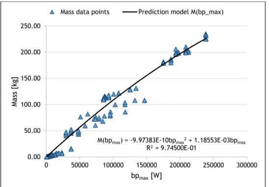
Figure 3.5 Engine mass relation with rated power, 𝑏𝑝𝑚𝑎𝑥, for 197 IC engines ... 50

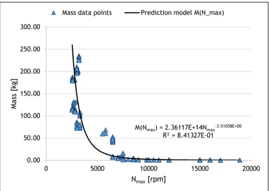
Figure 3.6 Engine mass relation with rated speed, 𝑁𝑚𝑎𝑥, for 197 IC engines ... 51

Figure 3.7 Deviation of the predicted engine mass values from the real data values... 52

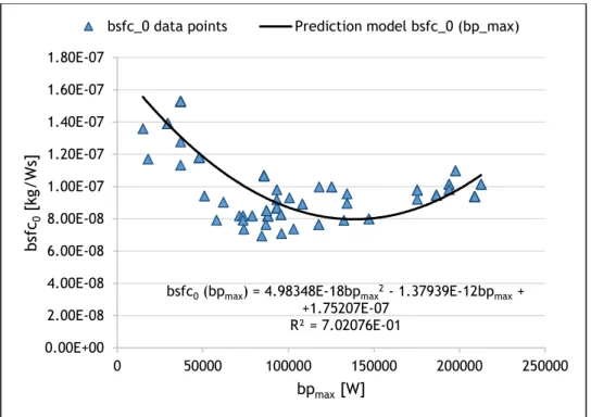
Figure 3.8 Engine maximum specific fuel consumption, 𝑏𝑠𝑓𝑐0, with rated power, 𝑏𝑝𝑚𝑎𝑥, for 118 engines ... 52

Figure 3.9 Engine maximum fuel consumption 𝑓𝑐0, with rated power, 𝑏𝑝𝑚𝑎𝑥, for 118 IC engines ... 53

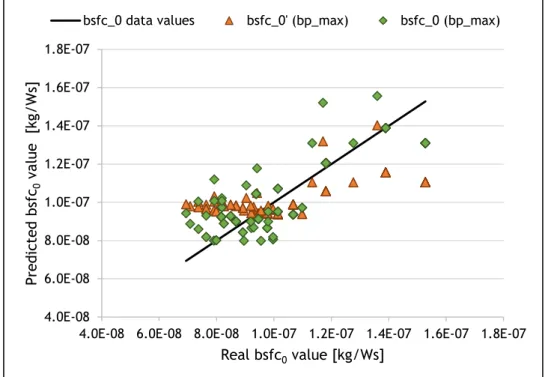
Figure 3.10 Deviation of the predicted 𝑏𝑠𝑓𝑐0 values from the real data values ... 54

Figure 3.11 Motor mass relation with maximum allowed current, 𝐼𝑚𝑎𝑥, for 294 electric motors ... 55

Figure 3.12 Motor mass relation with motor speed constant, 𝐾𝑣 for 294 electric motors ... 55

Figure 3.13 Deviation of the predicted motor mass values from the real data values ... 56

Figure 3.14 Motor resistance relation with maximum allowed current, 𝐼𝑚𝑎𝑥, for 265 electric motors ... 57

Figure 3.15 Deviation of the predicted motor resistance values from the real data values ... 57

Figure 3.16 Motor no load current relation with motor resistance, 𝑅, for 158 electric motors 58 Figure 3.17 Motor no load current relation with maximum current, 𝐼𝑚𝑎𝑥, for 158 electric motors ... 59

Figure 3.18 Deviation of the predicted motor no load current values from the real data values ... 60

Figure 3.19 Required current and engine speed for different mission stages ... 61

Figure 4.1 Convergence of the objective function, for case 1, into a stabilized solution for the LEEUAV according to the number of iterations ... 73

Figure 4.2 Convergence of 𝐾𝑣, for case 1, into a stabilized solution for the LEEUAV during the iteration process ... 73

Figure 4.3 Convergence of 𝐼𝑚𝑎𝑥, for case 1, into a stabilized solution for the LEEUAV during the iteration process ... 74

Figure 4.4 Convergence of the propeller design variables, for case 1, into a stabilized solution for the LEEUAV during the iteration process... 74

Figure 4.5 Gradient convergence to zero, for case 1 ... 75

Figure 4.6 Convergence of the objective function, for case 1, into a stabilized solution for the Hoji during the iteration process ... 80

Figure 4.7 Convergence of 𝑏𝑝𝑚𝑎𝑥, for case 1, into a stabilized solution for the Hoji during the iteration process ... 80

Figure 4.8 Convergence of 𝑁𝑚𝑎𝑥, for case 1, into a stabilized solution for the Hoji during the iteration process ... 81

Figure 4.9 Convergence of the propeller design variables, for case 1, into a stabilized solution for the Hoji during the iteration process ... 81

(17)

(18)

(19)

List of Tables

Table 3.1 Squared deviation sum for the three different mass empirical models analyzed ... 51

Table 3.2 Squared deviation sum for the two different 𝑏𝑠𝑓𝑐0 empirical models analyzed .... 54

Table 3.3 Squared deviation sum for the three different motor mass empirical models analyzed ... 56

Table 3.4 Squared deviation sum for the three different motor 𝐼0 empirical models analyzed ... 59

Table 4.1 LEEUAV data... 68

Table 4.2 Original LEEUAV electric motor data ... 68

Table 4.3 LEEUAV battery data... 68

Table 4.4 Original LEEUAV propeller data ... 69

Table 4.5 Mission waypoints ... 69

Table 4.6 LEEUAV loiter requirements ... 69

Table 4.7 LEEUAV mission constraints, defined by the user. ... 69

Table 4.8 LEEUAV mission parameters, defined by the user. ... 70

Table 4.9 Design constraints for the LEEUAV ... 70

Table 4.10 LEEUAV cases of study ... 71

Table 4.11 LEEUAV mission solutions ... 71

Table 4.12 LEEUAV mission performance solutions ... 71

Table 4.13 Selected motor from the optimized empirical results from case 1 ... 71

Table 4.14 HOJI data ... 76

Table 4.15 HOJI mission waypoints ... 76

Table 4.16 HOJI loiter requirements ... 76

Table 4.17 Hoji mission constraints, defined by the user ... 77

Table 4.18 Hoji mission parameters, defined by the user ... 77

Table 4.19 Design constraints for the Hoji UAV ... 77

Table 4.20 Hoji cases of study... 78

Table 4.21 Hoji mission solutions ... 78

Table 4.22 Hoji mission performance solutions ... 78

Table 4.23 Selected engine from the optimized empirical results from case 1 ... 78

Table A-I. Index of each IC engine name………...90

Table A-II. IC engine specifications data table………...94

Table B-I. Index of each electric motor name...99

(20)

(21)

Acronyms

UAV Unmanned Aerial Vehicle IC Internal Combustion EC External Combustion MBT Maximum Brake Torque

SI Spark Ignition

CI Compression Ignition

CG Conjugate Gradient

RC Radio Controlled

FFSQP FORTRAN Feasible Sequential Quadratic Programming SQP Sequential Quadratic Programming

(22)

(23)

Nomenclature

𝑎 Acceleration [ 𝑚 𝑠_{⁄ ]}2

𝑏𝑠𝑓𝑐0𝑑𝑎𝑡𝑎 Data Value for Brake Specific Fuel Consumption at 𝛿 = 1 [𝑘𝑔/𝑊𝑠]

𝑏𝑠𝑓𝑐0 Brake Specific Fuel Consumption at 𝛿 = 1 [ 𝑘𝑔 𝑊. 𝑠 ⁄ ]

𝑏𝑝𝑚𝑖𝑛 Minimum brake power (idle) [ 𝑊 ]

𝑏𝑝𝑆𝐿 Brake Power at Sea Level [ 𝑊 ]

𝑏𝑝 Brake Power [ 𝑊 ] 𝑏𝑠𝑓𝑐 Brake Specific Fuel Consumption [𝑘𝑔 𝑊. 𝑠⁄ ] 𝐶𝐷_𝑖 Drag Coefficient Vector

𝐶𝐷 Drag Coefficient

𝐶𝐿𝑇𝑂 Takeoff Lift Coefficient

𝐶𝐿 Lift Coefficient

𝐶𝑃₀ Propeller Power Coefficient at Null Advance Ratio 𝐶𝑝 Propeller Power Coefficient

𝐶𝑡 Propeller Thrust Coefficient

𝐷𝑖 Updated Propeller Diameter [𝑚] 𝐷𝑜𝑟𝑖𝑔𝑖𝑛𝑎𝑙 Original Propeller Diameter [𝑚] 𝐷𝑇𝑂 Takeoff Drag Force [𝑁] 𝐷 Propeller Diameter [𝑚]

𝐷 Drag Force [𝑁]

𝑑𝑇 Temperature Deviation from 𝑇0 [𝐾]

𝐸𝑚 Total Mission Energy [𝐽]

𝐹𝑅 Resulting Force [𝑁]

𝑓𝑐0 Maximum Fuel Consumption [𝑘𝑔 𝑠⁄ ]

𝑓𝑐 Fuel Consumption [𝑘𝑔 𝑠⁄ ]

𝑔 Gravity acceleration constant [ 𝑚 𝑠_{⁄ ]}2

ℎ𝑅𝐶 Defined altitude to calculate 𝑅𝐶𝑚𝑎𝑥 [𝑚]

ℎ𝑡𝑢𝑟𝑛 Defined altitude to calculate 𝛿𝑡𝑢𝑟𝑛 [𝑚]

ℎ𝑉_𝑚𝑎𝑥 Defined altitude to calculate 𝑉𝑚𝑎𝑥 [𝑚]

ℎ𝛾 Defined altitude to calculate 𝜃𝛾𝑚𝑎𝑥 [𝑚]

ℎ Altitude [𝑚]

𝐼𝑚𝑎𝑥′ Mission Maximum Required Current [𝐴]

𝐼0𝑑𝑎𝑡𝑎 Data Value for No Load Current [𝐴]

𝐼𝑚𝑎𝑥

𝑑𝑎𝑡𝑎 Data Value for Maximum Current [𝐴]

𝐼0 No load Current [𝐴] 𝐼𝑒𝑓𝑓 Motor Effective Current [𝐴]

(24)

𝐼 Input Current [𝐴]

𝑖 Current value

𝑖 + 1 Following value

𝑖𝑝 Indicated Power [ 𝑊 ] 𝐽𝑚𝑎𝑥 Maximum Propeller Advance Ratio

𝐽 Propeller Advance Ratio

𝐾𝑡 Motor Torque Constant [ 𝑁𝑚 𝐴⁄ ] 𝐾𝑣 Motor speed constant [ 𝑟𝑝𝑚 𝑉⁄ ]

𝐿 Lift Force [𝑁]

𝑚̇𝑓 Fuel flow per unit of time [ 𝑘𝑔 𝑠⁄ ]

𝑀𝑒𝑛𝑔𝑖𝑛𝑒_𝑖 Updated Engine Mass [𝑘𝑔]

𝑀𝑝𝑟𝑜𝑝𝑖 Updated Propeller Mass [𝑘𝑔]

𝑀𝑎𝑖𝑟𝑐𝑟𝑎𝑓𝑡 Aircraft Mass [𝑘𝑔]

𝑀𝑑𝑎𝑡𝑎 Data Value for Engine Mass [𝑘𝑔]

𝑀𝑒𝑛𝑒𝑟𝑔𝑦 Energy Mass [𝑘𝑔]

𝑀𝑜𝑟𝑖𝑔𝑖𝑛𝑎𝑙 𝑒𝑛𝑔𝑖𝑛𝑒𝑠 Original Engine Mass [𝑘𝑔]

𝑀𝑜𝑟𝑖𝑔𝑖𝑛𝑎𝑙 𝑝𝑟𝑜𝑝 Original Propeller Mass [𝑘𝑔]

𝑀𝑝𝑎𝑦𝑙𝑜𝑎𝑑 Payload Mass [𝑘𝑔]

𝑀𝑠𝑡𝑟𝑢𝑐𝑡𝑢𝑟𝑒 Aircraft Structure Mass [𝑘𝑔]

𝑀𝑠𝑦𝑠𝑡𝑒𝑚𝑠 Aircraft Systems Mass [𝑘𝑔]

𝑀 Mass [𝑘𝑔]

𝑁𝑚𝑎𝑥′ Mission Maximum Required Engine Speed [𝑟𝑝𝑚]

𝑁𝑚𝑎𝑥

𝑑𝑎𝑡𝑎 Data Value for Maximum Engine Speed [𝑟𝑝𝑚]

𝑁𝑚𝑖𝑛 Minimum Engine Speed [𝑟𝑝𝑚]

𝑛𝑒𝑛𝑔𝑖𝑛𝑒 Number of engines 𝑛𝑙𝑖𝑚𝑖𝑡 Limit Load Factor

𝑛𝑙𝑜𝑎𝑑 Load Factor

𝑛𝑢𝑙𝑡𝑖𝑚𝑎𝑡𝑒 Ultimate Load Factor

𝑁 Rotational Speed [ 𝑟𝑝𝑚 ]

𝑁 Normal Reaction Force [𝑁]

𝑃𝑠ℎ𝑎𝑓𝑡 Motor Shaft power [ 𝑊 ]

𝑝𝑖 SQP algorithm step direction

𝑝 Propeller Blade Pitch [𝑚] 𝑄 Engine Torque [ 𝑁𝑚 ] 𝑅𝐶𝑚𝑎𝑥_𝑟𝑒𝑓 Constraint Reference for Maximum Rate of Climb [ 𝑚 𝑠⁄ ] 𝑅𝐶𝑠𝑐𝑚𝑖𝑛 Constraint Reference for Maximum Rate of Climb at ℎ𝑠𝑐 [ 𝑚 𝑠⁄ ]

𝑅𝑑𝑎𝑡𝑎 Data Value for Electric Resistance [Ω]

(25)

𝑅𝑈 Battery Internal Resistance [Ω]

𝑅Ω Motor Speed Controller Resistance [Ω]

𝑅 Motor Resistance [Ω]

𝑅 Universal Gas Constant [ 𝐽 𝑘𝑔. 𝐾⁄ ]

𝑅 Friction Force [𝑁]

𝑅𝐶 Rate of Climb [ 𝑚 𝑠⁄ ]

𝑟𝑐 Compression Ratio

𝑆𝑇𝑂_𝑟𝑒𝑓 Constraint Reference for Ground Roll [𝑚]

𝑆𝑔 Ground Roll [𝑚]

𝑆 Wing Surface Wet Area [𝑚2_]

𝑠𝑓𝑐 Specific Fuel Consumption [𝑘𝑔 𝑊. 𝑠⁄ ]

𝑇𝑅𝑚𝑖𝑛 Minimum Required Thrust [𝑁]

𝑇0 Standard Sea Level Temperature [𝐾]

𝑇𝐴 Propeller Available Thrust [𝑁]

𝑇𝑅 Required Thrust [𝑁]

𝑇𝑇𝑂 Takeoff Thrust [𝑁]

𝑡𝑇𝑂 Takeoff Time [𝑠]

𝑇 Air Temperature [𝐾]

𝑡 Time [𝑠]

𝑈𝑒𝑓𝑓 Back Electromotive Voltage [𝑉] 𝑈 Input Voltage [𝑉]

𝑉𝑆𝑡𝑢𝑟𝑛 Stall Speed at Level Turn [ 𝑚 𝑠⁄ ]

𝑉∗ _{Maneuver Speed} _{[ 𝑚 𝑠}_{⁄ ]}

𝑉𝐵𝐶 Best Rate of Climb Speed [ 𝑚 𝑠⁄ ]

𝑉𝐷 Dive Speed [ 𝑚 𝑠⁄ ]

𝑉𝐻 Horizontal Component of Speed [ 𝑚 𝑠⁄ ]

𝑉𝑆 Stall Speed [ 𝑚 𝑠⁄ ]

𝑉𝑇𝑂 Takeoff Speed [ 𝑚 𝑠⁄ ]

𝑉𝑑 Displacement Volume [ 𝑚3 ] 𝑉𝑚𝑎𝑥_𝑟𝑒𝑓 Constraint Reference for Maximum Allowed Speed [ 𝑚 𝑠⁄ ]

𝑉𝑚𝑎𝑥 Maximum Allowed Speed [ 𝑚 𝑠⁄ ]

𝑉𝑚𝑖𝑛 Minimum Allowed Speed [ 𝑚 𝑠⁄ ]

𝑉𝑡𝑢𝑟𝑛 Air Speed at Level Turn [ 𝑚 𝑠⁄ ]

𝑉 Air speed [𝑚 𝑠⁄ ]

𝑊𝑎𝑖𝑟𝑐𝑟𝑎𝑓𝑡𝑖 Updated Aircraft Weight [𝑁]

𝑊𝑓𝑢𝑒𝑙 Fuel Weight Consumed [𝑁]

𝑊𝑡𝑢𝑟𝑛 Aircraft Weight at Level Turn [𝑁]

𝑊 Aircraft Weight [𝑁]

(26)

Δ𝑡𝑖 Mission Segment Duration [𝑠] Φ Rolling Angle [°] Ω Motor Speed [𝑟𝑝𝑚] 𝛼̅ Coefficient Vector of the 𝐶𝑝 Equation

𝛼𝑖 SQP algorithm step length

𝛼 Temperature Increment per Meter Climbed Below Tropopause [℃ 𝑚⁄ ] 𝛽̅ Coefficient Vector of the 𝜂𝑝 Equation

𝛾̅ Coefficient Vector of the 𝐽𝑚𝑎𝑥 Equation

𝛾𝑚𝑎𝑥_𝑟𝑒𝑓 Maximum Rate of Climb Angle Constraint Reference [°] 𝛾𝑚𝑎𝑥 Maximum Rate of Climb Angle [°] 𝛾 Rate of Climb Angle [°] 𝛿′𝑚𝑎𝑥 Mission Required Throttle

𝛿𝑡𝑢𝑟𝑛 Engine Throttle for a Sustained Turn

𝛿 Engine Throttle

𝜀̅ Coefficient Vector of the 𝐶𝑝₀ Equation 𝜀 SQP Algorithm Tolerance Error

𝜁̅ Coefficient Vector of the 𝜂𝑚𝑎𝑥 Equation

𝜂𝑚𝑎𝑥 Maximum Propeller Efficiency 𝜂𝑝 Propeller Efficiency

𝜂 Motor Efficiency

𝜃𝑝𝑖𝑡𝑐ℎ Blade Chord Angle [°] 𝜇 Friction Coefficient

𝜌0 Air density at Sea Level [𝑘𝑔 𝑚⁄ 3] 𝜌 Air density [𝑘𝑔 𝑚_⁄ 3_] 𝜔 Angular Velocity [ 𝑟𝑎𝑑/𝑠 ]

(27)

(28)

(29)

1 Introduction

1.1 Motivation and Focus

Since the beginning of the 20th_{century, when the first developments in aeronautical sciences}

started and the first airplanes were constructed, engineers have always tried to improve aircraft performance, while simultaneously diminishing its energy consumption. This is a continuous aim throughout history, as men possess a need to improve and perfect any scientific work which may be useful, serviceable and profitable to the overall community. Hence aircraft optimization is a highly studied field, in order to find the best design conditions which grant the best possible outcome.

However, optimizing the innumerous design variables which condition an aircraft, no matter its size, proves to be quite challenging. At a designing phase, all parameters interrelate, having oftentimes inverse relations with each another. This means changing a variable at a certain field may considerably affect another at a seemingly unrelated section. Thus optimizing an aircraft design parameters requires a multi-disciplinary optimization which takes into account various different dependent variables.

Aircraft optimization may prove very costly in terms of time and calculations, but in the last decades it has been specially improved, due mostly to the improved technology and resources provided by many different computer simulators. Therefore, after the creation of optimization algorithms which facilitated immensely the analysis between the various relations of the design variables, in relation to a certain objective function, many optimization softwares were created. Still, the majority of them only consider one simple condition, like one fixed altitude, or one single stage of flight. Optimizing an aircraft for an entire operating mission which considers the whole flight envelope is a much more ambitious goal. Mission optimization softwares are not so easily available and are much scarcer. Henceforward, in this dissertation the performance of an aircraft will be optimized for a full operating mission, and for the resulting optimized solution it will be found the most suitable propulsion system in order to minimize the total energy spent.

1.2 Objectives

In this dissertation, an already existing optimization software was used to minimize the total energy consumed during a given mission, for two types of aircraft. One is powered by an electric motor, and another by an internal combustion engine. In order to do so, several modifications and additions must be introduced in the program. It is necessary to match a suitable propulsion system to the optimum solution given by the software. This optimum solution is the minimization of the objective function, i.e. the total mission energy consumed. The software

(30)

returns the optimized design values for the propeller diameter and pitch, but only for a fixed engine.

Since the optimization algorithm has the ability to optimize the design variables that the user chooses to input, in this thesis the engine design parameters are added into the algorithm, and the resulting solution returns not only the optimized propeller diameter and pitch, but also the matching engine parameters.

Therefore, it is necessary to create two data bases, one for the electric motor and another for the internal combustion engine, with a large number of data elements. Then, the relations between all the engine/motor variables are analyzed and investigated, in order to obtain certain empirical functions. These functions should return the engine specifications, dependent on one or more parameters. These parameters would then become the design variables, or in other terms the abscissas of the objective function, and all engine related calculations inside each iteration of the algorithm use these empirical models.

When the algorithm displays the final solution for a minimum value of the objective function, it returns also the optimized design specifications of the engine, and so the engine selection will be made from the database created. The engine selected is the one most similar to the empirical models solution.

Another addition to the program is the calculation of the mission performance variables inside the algorithm, to enable the user to constrain mission parameters (such at maximum speed or takeoff runway distance) and still obtain the intended minimum solution inside the feasible space.

To summarize, there are two main objectives in this dissertation, in order to fully improve the intended mission performance:

 To create two data bases, one for electric motors and another for internal combustion engines, in order to obtain the empirical engine models and verify if these models present satisfactory matches with the optimum solution.

 To add the performance mission parameters calculations into the algorithm, to enable the user to constrain them.

(31)

1.3 Dissertation Layout

This dissertation consists of five main parts. The first chapter introduces the focus and the objective of the thesis, and presents a very brief literature review concerning optimization algorithms and some concepts related to the combustion engine and the electric motor. The second chapter presents an overview on aircraft performance theory. More precisely, it presents the engine and propeller performance mathematical models which are used in the software calculations, and the mission performance model that is to be added.

The third chapter presents the methodology concerning the programing procedures applied. In further sections, it presents the engine data bases created and the empirical models obtained, which were then introduced in the software. The mission performance calculations and constraints added to the program are also discriminated in the final section of this chapter. Chapter four presents the optimized results for two different cases of study, by applying the engine empirical models obtained for certain mission restrictions imposed, and verifying if the models present satisfactory matches. One case of study is analyzed for an UAV powered by an electric motor, and the other for an UAV powered by an IC engine.

Chapter five presents the conclusions of the overall analysis and reflects if the objectives defined in section 1.3 were met, presenting some considerations regarding future works.

(32)

1.4 Literature Review

The invention of the engine was one of the most noteworthy events in history, as it improved significantly the distance in which vehicles could travel with much less effort and much more convenience. It is defined as a mechanical engineering device that converts one form of energy into a mechanical work, which is used to produce a pushing force called thrust [1]. Thus the engine propels a certain vehicle into movement, whether it is an automobile, a ship, a space shuttle or an aircraft. Among the many types of engines used in aircraft propulsion systems, two of the most relevant are the internal combustion engine and the electric motor.

Since the performance of the engine/motor greatly influences the overall performance of the mission, properly selecting an engine to match a certain airframe and propeller is vital to an optimized flight performance. Hence, and taking advantage of the nowadays technology, many computational optimization procedures and analysis software are used to improve aircraft design. Optimizing the performance of an aircraft requires the use of intense computational simulation, in order to design and analyze complex systems that interact with one another. Consequently, it is essential to understand what optimization is, as well as what types of different computational methods were developed. Thus below follows a brief summary on the state of computational simulation in aircraft design, an overview on different types of optimization algorithms and lastly, some concepts and classifications regarding the IC engine and the electric motor.

1.4.1 Brief summary on modeling and aircraft design optimization

Before 1960, the development and analysis of aerodynamic configurations relied mostly on practical experiments and wind tunnel tests. As technology improved, computational methods provided better numerical algorithms, capable of performing faster and improved optimization techniques. These were, from there on, applied frequently to aircraft design optimization problems [2], since many formed a system too costly in time and means to analyze without the aid of computer processing. Researchers were then allowed to analyze phenomena which were before too complex to model. Exemplifying, in 1978, Raymond M. Hicks and C. A. Szelazek [3] were able to optimize an airfoil through a numerical optimization using a minicomputer. Later in the 1980s, Gary B. Cosentino and Terry L. Holst [4] performed a study on transonic wing configurations, using, likewise, a numerical optimization process through computational simulation. Computational science started then to become indispensable for the aircraft industry, and was greatly developed in multidisciplinary optimization in the 1990s [5].

When defining design optimization problems, it is important to properly select the objective function in order to achieve the intended performance [2]. Many objective functions were analyzed in previous works. For instance, reducing the maximum takeoff weight or reducing the aircraft operation costs [6, 7] are two examples. However, finding an optimization which considers the entire mission and flight envelope is indeed quite difficult. Most optimizations

(33)

are performed at a single flight condition. However, aircrafts are designed to fly different missions at different flight circumstances, such as altitude, speed and available throttle. Hence, it is essential to optimize the performance of an aircraft under multiple mission flight conditions. An efficient and accurate mission analysis procedure is therefore required to realistically model aircraft performance in optimization problems [2]. When formulating a problem, it must always be taken into consideration the decision variables, the restrictions and the objective function. Modeling the objective function in order to maximize it or minimize it is very complex, as the many parameters affecting the performance present interdependencies between them. Hence there must always exist a balance between the various input parameters.

1.4.2 Overview on optimization algorithms

Optimization has a wide variety of applications and it is implemented in almost every scientific field, such as engineering, physics, management and design. Such wide scope of uses exists due to the need of obtaining the best solution for a given problem, without wasting more than the necessary means and time [8]. This makes optimization much more important in the resolution of practical procedures rather than theoretical problems [9]. In some fields, the main goal may be to minimize the cost of a certain product, the fuel consumption of a vehicle or the energy consumption of an equipment. Else it may be to maximize a certain characteristic like the profit of a company.

However determining the optimal use of the available resources may prove a challenge, since real world issues present complex parameters and technical features which are too elaborate to formulate. With the amount of complexity and variables that can be presented at a stated problem, computational calculations is almost always required, since it efficiently allows the analysis of more complex and apparently aleatory problems. Therefore in the last century, computational optimization algorithms have been developed and studied [10].

To start the resolution of the problem in study, an optimal procedure is employed, which consists of three main parts: modeling, choosing the algorithm and running the simulator. The representation of the physical problem through a set of mathematical equations, which can be solved numerically, is the modeling phase of the problem. Then, at a later stage, it is necessary to select the appropriate algorithm according to the mathematical characteristics of the problem. Finally, it is selected a computational simulator capable of performing the calculation and evaluating if the proposed solution is optimal and doable [10]. Fig. 1.1 represents a graphical scheme of an optimization procedure.

Figure 1.1 Optimization Process

Mathematical

(34)

Although there are several ways to formulate the problem in the modeling phase, the most widely method used is to write it as a minimization of a function or a set of functions, subject to a series of constraints [10], in a manner such as

𝑀𝑖𝑛𝑖𝑚𝑖𝑧𝑒 𝑓𝑖(𝑥𝑛), (𝑖 = 1,2, … , 𝑀)

subject to a set of constraints like, for example,

ℎ𝑗(𝑥𝑛) = 0, (𝑗 = 1,2, … . , 𝐽)

𝑔𝑘(𝑥𝑛) ≤ 0, (𝑘 = 1,2, … , 𝐾)

where 𝑓𝑖(𝑥), ℎ𝑗(𝑥) and 𝑔𝑘(𝑥) are in general nonlinear functions and the vector (𝑥1, 𝑥2, … , 𝑥𝑛) can be continuous or discrete. The function 𝑓𝑖(𝑥𝑛) is called the objective or cost function, since it is the property that one wants to optimize. This formulation can also be written as a maximization by simply replacing 𝑓𝑖(𝑥𝑛), with −𝑓𝑖(𝑥𝑛) [10]. Thus, this allows the simplification of a physical attribute, translating it into a set of numerical equations. The objectives, variables and restrictions are all identified in this phase, and the choice of the most effective algorithm depends on a good and efficient mathematical formulation, in order to ensure the minimized solutions are reachable.

There is no universal algorithm which can solve every problem. Finding the correct one depends on the properties of the problem which is being analyzed [11]. Optimization algorithms can be classified in many different ways. They may depend on the type of function (linear, nonlinear, restricted or unrestricted), the type of variables (continuous or discrete), the techniques employed (deterministic, hybrid or stochastic), the solution desired (global or local optimization) or if the minimization relies or not in the knowledge of derivatives/gradients [12].

Gradient-based algorithms, like the Gauss-Newton method [10], use the derivative information. Generally the most common used method, since it requires a lower number of evaluations of the objective function, and therefore a low computational cost. In contrast, gradient-free based algorithms, like the downhill simplex method [13], do not use the derivative information which will result in more complex calculations and a higher number of evaluations. It has a high computational cost and is used when the objective function is non-differentiable or it is trapped in a local minimum.

Deterministic algorithms work in a mechanical and deterministic manner, without any random nature. Downhill simplex and hill climbing methods are good examples of deterministic algorithms that will reach the same final solution if they start with the same initial point.

(35)

However, if every time the algorithm runs with the same starting point, it presents a different solution, it means there is some randomness to its nature. Genetic algorithms or hill climbing with random restart are classified as stochastic algorithms, due to the random nature associated with the results they generate [14].

Some problems require mixed-type or hybrid algorithms. They use the combination of deterministic methods and randomness, in order to achieve a more suitable solution to the case in study. Genetic algorithms may be hybridized with others, modifying some components of the other algorithm and creating a more efficient method to the specific problem.

From another perspective, if the algorithm converges to a local optimum and not the global one, it is classified as a local search algorithm. Most deterministic methods like hill climbing are also local methods since it is sometimes very hard to determine the global optimum and instead, given a set of constraints, it is possible to achieve a satisfying local optimum for a particular case. If, however, some random restart is inserted to a hill climbing algorithm, it changes from a local to a global search algorithm. This means randomness is a crucial factor in global search methods [14].

Another important matter to focus upon is the complexity that some objective functions may present. Non-differentiable functions that many times are generated from computer simulations, present a very high computational cost and difficult calculations. In this cases straightforward optimization of the cost function is not advisable. Hence, it is better to construct from the sample data of the objective function a mathematical model which substitutes the original one, being the most similar as possible and yet simpler. This new model is easier to optimize, but it must still be reasonably accurate so it can produce predictions and solutions like the original objective function. This is the surrogate based algorithm [15]. There is indeed a wide variety of optimization methods to be selected, and sometimes a combination of various algorithms may prove the best option. This highly depends on the restrictions and mathematical properties of the problem, so the selection of the algorithm is a significant phase that must be carefully weighted.

1.4.2.1 Conjugated gradient algorithm

Derivative-based or gradient-based algorithms use the information of the function derivatives. Such algorithms should not be selected if there is discontinuity in the objective function, which makes it a non-differentiable equation and therefore, may render such methods unsuitable [10]. The most well-known classical methods are the Newton’s Method and Hill-Climbing, while more modern approaches use algorithms like the conjugate gradient (CG) method, the steepest descent method or the Broyden–Fletcher–Goldfarb–Shanno (BFGS) method. Gradient-based algorithms are therefore widely used in discrete modelling [10, 16]. Since detailed

(36)

mathematical explanation about gradient-based algorithms is not the main focus of this dissertation, only a brief account on its particulars is presented below.

Gradient based methods use the gradient vector of the objective function, which gives the partial derivatives with respect to each of the independent input parameters. In a sense it is the slope of the tangent line to the objective function at a certain point (design parameter value), and equals zero at the minimum of the objective function, which is the desired solution. The derivative of a function also indicates in which direction the function is decreasing or increasing. A partial derivative (gradient) less than zero corresponds to a decrease in the objective function, and therefore the algorithm has the direction in which to search for the minimum. However, the objective function must be non-convex or else the algorithm would be trapped in a local minimum [17], as illustrated below.

Figure 1.2 Non-convex function [18]

A gradient measures how much the output of a function changes if one changes the inputs in small proportions. The higher the gradient, the higher and steeper the slope is in the objective function. One common analogy used for better understanding is a descent into the bottom of a valley. Exemplifying, the objective is to be exactly at the bottom point of a valley in the minimum amount of time possible, without knowing, however, its exact location. In the starting point of the valley descent, one would start taking larger portions of the steepest path towards the bottom to save time, and as it approaches the final objective it would take less steep paths as it would slowly search and converge into the lowest point. A similar process occurs with gradient based algorithms. The higher the slope value, or in better terms the gradient value, the faster the algorithm learns and progresses rapidly, and as it goes nearer to the intended optimum point it assumes smaller gradient values, as it converges to zero and therefore to the solution. Henceforth, the gradient vector takes a descendent path towards the solution, assuming smaller and smaller values. This phenomenon is also designated as the gradient descent, which can prove to be quite slow in many occasions. Gradient descent is a minimization process that minimizes the Hessian matrix (matrix which contains all gradients) of the objective function, ∇𝑓𝑖(𝑥𝑛). Both the steepest descent method and the conjugate gradient method (CG) present this gradient descent. The difference is that the CG based method in particular, takes into account the history of the gradients to move more directly

(37)

towards the optimum. Each descent direction is modified by adding a contribution from the previous direction/gradient [17]. The figures below better clarify the process, assuming an objective function 𝑓(𝑥1, 𝑥2) with the input parameters defined as 𝑥1 and 𝑥2.

Figure 1.5 3D representation of 𝑓(𝑥1, 𝑥2)[19]

Note that in this graphical representations, the parameter variables 𝑥1 and 𝑥2 are not subjected to any constraints, so there is not a feasible space defined. A feasible space is a space where the independent variables are defined within certain constraints [20]. So if there is no local minimum inside this space, the solution is not feasible and there would not exit a feasible region for the minimum desired. Additionally, if there is indeed a local minimum, the gradients of the function would not converge to zero (since it is not the global minimum) but to the minimum solution possible given the constraints applied. Thus, it is important to consider what constraints values to apply to the problem and avoid design requirement bounds which impose too tight limits for the feasible space.

Defining the feasible space within reasonable values, given the context of the problem to optimize, is an important step towards an efficient optimization process. Conclusively, a

Figure 1.3 2D representantion of the solution path of

(38)

gradient based algorithm will begin at certain starting design values, 𝑥𝑛. Then it searches for the minimum solution desired between a set of 𝑥𝑛 values defined by an upper boundary and a lower boundary, i.e. 𝑙𝑜𝑤𝑒𝑟 ≤ 𝑥𝑛≤ 𝑢𝑝𝑝𝑒𝑟. Lastly, the optimum solution is then achieved if the gradients of the objective function, i.e. ∇𝑓𝑖(𝑥𝑛), converge to zero or to a very small tolerance error, 𝜀, near zero.

1.4.3 Internal combustion engine: concepts and classifications

According to Williard W. Pulkrabek [1], the internal combustion engine is a heat engine that converts chemical energy in a fuel into mechanical energy, usually made available on a rotating output shaft. The chemical energy of the fuel is first converted to thermal energy, by means of a combustion process or oxidation, with air inside the engine. This thermal energy raises the temperature and pressures of the gases within, and the high pressure gas then expands against the mechanical mechanism of the engine. This expansion is converted by the linkages of the engine to a rotating crankshaft. The crankshaft, in turn, is connected to a transmission which transmits the mechanical output work to the desired final use. This will often mean the propulsion of a vehicle, such as automobiles, marine vessels or aircrafts [1].

A combustion that takes place inside the engine system is designated as internal combustion (IC) engine. Early in the latter half of the 1700s, heat engines, including external combustion and internal combustion engines, suffered major developments due to the emerging of the railroad locomotive. However, drastically improvements of the IC engine occurred only in the latter half of the 1800s, with the invention of the automobile. Nowadays, different manufactures have produced many distinct IC engines which vary in size, geometry, style and operating properties. Most IC engines are reciprocating engines, due to the reciprocating motion of the pistons within the cylinders, which can be arranged in many different configurations. Reciprocating engines are classified depending on different criteria. Commonly, they are more frequently differentiated depending on the type of ignition and the type of engine cycle. Thus, they may be classified as spark ignition engines (SI) or as compression ignition engines (CI), and either of these two types may be classified as a two stroke engine or a four stroke engine [21].

In SI engines the combustion process of the fuel, at each cycle, occurs by a spark generated by the spark plug, located in the cylinder head of the engine. The fuel used is gasoline or petrol. The engine works on the basis of a constant volume heat addition cycle, also known as Otto cycle [21]. Not only an ignition system is necessary, but also a carburetor responsible for mixing the air and fuel that is afterwards introduce in the cylinder through the suction stroke. In CI engines, the combustion process of the fuel starts when the air fuel mixture self-ignites due to high temperature in the combustion chamber, caused by high compression [1]. The fuel used is Diesel, since it has a low self-ignition temperature when compared to gasoline.

(39)

Important to note that CI engines are also comparatively heavier due to higher peak pressures required [22]. The engine works therefore on a basis of a constant pressure heat addition cycle, also known as Diesel cycle. CI engines have a fuel injector and a fuel pump, since fuel is injected directly into the combustion chamber at high pressure.

SI and CI engines are either two stroke or four stroke engines. In four stroke engines the thermodynamic cycle, in order to produce one power stroke, is completed in four strokes of the piston or two revolutions of the shaft. In two stroke engines the thermodynamic cycle, in order to produce one power stroke, is completed in two strokes of the piston or one revolution of the shaft [22]. Comparing the two, four stroke engines have higher efficiencies for every cycled completed. Two stroke engines tend to produce more power for the same size of engine, or rather the same amount of power for lighter and more compact engines [22].

1.4.4 Electric motor: concepts and classifications

Electric motors are being used more frequently, since they are overall more reliable and require less maintenance cares. An electric motor is a device which converts electric energy shaft power. They operate according to the interaction between the motors magnetic field and current, in order to generate a rotational force. The link between electricity, magnetism, and movement was originally discovered in 1820 by French physicist André-Marie Ampère (1775– 1867) and later developed by Englishmen Michael Faraday (1791–1867). When an electric current flows through a wire, it creates a certain magnetic field. If the wire is near a permanent magnet, which has its own magnetic field, the two fields will interact with each other and create a repelling or attracting motion [23]. The direction of the motion is generated according to Fleming's Left-Hand Rule [24], where the second finger is the direction of the current, the first finger the direction of the magnetic field and the thumb the direction of the force. Furthermore, if a wire with a current flowing in one direction, is shaped like an U, then theoretically there are two parallel wires running through the magnetic field of the permanent magnet, each with current flowing in different directions. Then according to Fleming's Left-Hand Rule the two wires will move in opposite directions, one upward and the other downward, and a turning motion, i.e. torque, is thus created [23]. However, the coil of wire will not fully rotate. Once the coil reaches the vertical position and flips, the electric current would be flowing in the opposite direction, so the forces would also reverse. Instead of rotating continuously in the same direction it would move back and forward. Thus, for every half a turn of the coil, the direction of the electric current through the windings must be reversed. To overcome this problem, electric motors present different operating mechanism and are classified according to its component parts, connections and type of current. In brief, electric motors can be classified between AC motors and DC motors. Although AC and DC motors serve the same function of converting electrical energy into mechanical energy, they are powered,

(40)

constructed and controlled differently. AC motors use alternating current, i.e. a current which periodically reverses direction, and motor speed is controlled by frequency. DC motors operate with direct current and are powered by ion batteries. Motor speed is controlled by varying the current flux, which can be controlled by altering the applied voltage or resistance (through a speed controller resistance). DC motors are additionally classified as brushed or brushless. A brushed motor uses a direct current together with a component, named a commutator, placed in the ends of the coil, which is responsible for reversing the electric current each time the coil rotates through half a turn. Electric power is delivered from the battery into the commutator through a pair of loose connectors called brushes, and thus the coil will rotate continuously in the same direction. However, the commutator presents many disadvantages. Power losses occur due to friction between the brushes and the commutator, which wears down the soft brush material. This adds to maintenance costs and reduces the motor life expectancy, which justifies a decline in the use of brushed DC motors. With the development of electronics, brushless DC motors without a commutator or brushes were created. Contrarily to a brushed motor, the coils do not rotate and remain static, surrounding a permanent magnet. Since the coils do not move, there is no need for a commutator or brushes. Instead, by changing the direction of the magnetic fields generated by the stationary coils, the permanent magnet rotates. The rotation is controlled by adjusting the magnitude and direction of the current. Hence, brushless DC motors present increased reliability, life expectancy, efficiency and torque to weight ratio, and have therefore become a popular motor choice for RC aircraft models.

(41)

2 Performance Models

It is important to note that the electric motor and the internal combustion engines present very different performance parameters and mathematical models. A parameter is a numerical or other measurable factor, forming one of a set that defines a system and sets the conditions of its operation. Therefore the efficiency of the engine is restricted by certain performance parameters. Before analyzing the optimization procedure applied, a brief summary on the mathematical performance models already being used in the software for these two types of engines and for the propeller is presented below. Furthermore, the mission performance model which was added to the software is also latter presented.

2.1 Internal combustion engine performance model

Internal combustion engines typically work within a useful range of speed. The overall performance of the engine depends on the relation between the power developed, the engine rotational speed, 𝑁, and the specific fuel consumption at each operating condition, 𝑠𝑓𝑐, as depicted in the figure below [22].

Figure 2.1 Relation between IC engine performance parameters

In general, the energy that flows through the engine can be summarized in two different terms. They are the indicated power, 𝑖𝑝, and brake power, 𝑏𝑝. 𝑖𝑝 is the theoretical maximum output power of the engine, available from the expansion of the gases in the cylinders without taking into account any friction losses, heat losses or entropy within the system [22]. 𝑏𝑝 is the actual power available at the delivery point, the engine crankshaft, after taking into account energy losses in friction, pumping, and various other factors. It presents a more practical interest as it is responsible for delivering the rotational speed to the propeller. Fig. 2.2 presents graphical representation of the energy distribution inside the engine, for a better understanding.

Performance Power [𝑊] 𝑁 [𝑟𝑝𝑚] 𝑠𝑓𝑐 [𝑘𝑔 𝑊𝑠]⁄

(42)

Figure 2.2 Energy Distribution in the IC Engine [22]

Indicated power, 𝑖𝑝, is thus a measure of the forces that are developed within the cylinder. The actual useful power delivered by the engine, 𝑏𝑝, is a measure of the remaining power that effectively contributes to the rotational force at the shaft. [22].

Engine performance can be better analyzed through a set of operating charts which illustrate the performance of the engine, as well as its rating operating characteristics. Engine rating usually indicates the highest power at which the engine delivers a reasonably good performance. Generally, the factors evaluated are satisfactory economy, reliability, maximum power (𝑏𝑝𝑚𝑎𝑥) and durability under service conditions [22]. Since IC engines generally operate within a useful range of speed, 𝑁, there are various operating circumstances which should be considered, namely if it is a maximum or normal rated operation, or if it is a full load operation. Commonly normal rated power designates the highest power an engine is allowed to develop during continuous operation, and it is achieved at a wide-open throttle regime. As for maximum rated power, it is defined as the highest power an engine is allowed to develop during specific short periods of time, like the takeoff segment. Fig. 2.3 represents the dependence of brake power, 𝑏𝑝, torque, 𝑄, and 𝑏𝑠𝑓𝑐 as a function of engine speed, 𝑁.

Figure 2.3 Torque, brake power and brake specific fuel consumption as a function of engine speed [25]

(43)

Within the useful range of speed, power has a maximum usable value. The ratio between power available at a certain speed, 𝑁, to the maximum output power at this same speed is called load, 𝑏𝑝 𝑏𝑝⁄ 𝑚𝑎𝑥, or in other terms, engine throttle, 𝛿.

Another operating circumstance also frequently considered is the mission duration. For long periods of operation, the ideal parameter to optimize, instead of the 𝑏𝑝 and 𝑄, would be the engine brake specific fuel consumption, 𝑏𝑠𝑓𝑐. This would provide a greater operation time for the aircraft, since energy consumptions would be minimized. Analyzing Fig. 2.3, 𝑏𝑠𝑓𝑐 initially decreases with engine speed, 𝑁, since at this stage there is a shorter time period for heat losses to occur. Hence the fuel energy is more efficiently harnessed. However, for a higher 𝑁, 𝑏𝑠𝑓𝑐 again increases due to the increase in friction losses associated with high speeds.

The available engine throttle, 𝛿, also compromises 𝑏𝑠𝑓𝑐. The wider open the engine throttle is, the greater becomes the brake power available and thus 𝑏𝑠𝑓𝑐 will decrease, due to pumping losses for SI engines and constant friction losses that subtract from the indicated power, since 𝑖𝑠𝑓𝑐 remains fairly constant. This decrease in 𝑏𝑠𝑓𝑐 is illustrated in Fig. 2.4 [26].

Figure 2.4 Brake specific fuel consumption as a function of engine throttle [26]

All these graphical representations of engine performance are generally obtained through two different methods, whether by using experimental results obtained from engine experimental tests, or by analytical calculation based on theoretical data. Ultimately, the internal combustion engine performance can be described through a mathematical model. The equations used in this dissertation are thus presented below.

𝑏𝑝 is formulated through an approximated model translated by the linear regression illustrated in Fig. 2.5.

(44)

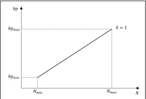
Figure 2.5 Approximated linear regression for 𝑏𝑝, at sea level and full load

Fig. 2.5 illustrates brake power at sea level conditions for wide-open throttle, 𝛿 = 1. Thus, the resulting linear equation for the presented model is given by

𝑏𝑝(𝑁) [𝑊] = 𝑏𝑝𝑚𝑖𝑛+ (𝑏𝑝𝑚𝑎𝑥− 𝑏𝑝𝑚𝑖𝑛 𝑁𝑚𝑎𝑥− 𝑁𝑚𝑖𝑛

) × (𝑁 − 𝑁𝑚𝑖𝑛) (2.1)

and since brake power is also a function of the available throttle, 𝛿, then at sea level 𝑏𝑝 is formulated as

𝑏𝑝𝑆𝐿(𝑁, 𝛿) [𝑊] = 𝛿 × 𝑏𝑝(𝑁) (2.2)

Altitude effects should also be taken into consideration. Mass flow into the engine is affected by the outside air density, which varies significantly with altitude. Thus, equation 2.4 accounts for the air density effects upon brake power according to reference [27], and is given by

𝑏𝑝 (𝑁, 𝛿, 𝜌) = 𝑏𝑝𝑆𝐿(𝑁, 𝛿) × ( 𝜌 𝜌0

−1 − 𝜌 𝜌0⁄

7.55 ) (2.3)

where 𝜌 is the air density in [𝑘𝑔 𝑚_⁄ 3_]_{and 𝜌}

0 the air density at sea level.

After calculating brake power, 𝑏𝑝, it is possible to obtain the available torque at the rotational shaft, 𝑄, knowing that

𝑄(𝑁, 𝛿, 𝜌) [𝑁𝑚] =𝑏𝑝(𝑁, 𝛿, 𝜌) 𝜔 (2.4) 𝛿 = 1 𝑁 𝑁𝑚𝑎𝑥 𝑁𝑚𝑖𝑛 𝑏𝑝𝑚𝑖𝑛 𝑏𝑝𝑚𝑎𝑥 𝑏𝑝

(45)

where 𝜔 is the angular velocity in [𝑟𝑎𝑑 𝑠⁄ ], formulated as 𝜔 [𝑟𝑎𝑑/𝑠] =2𝜋𝑁 60 (2.5) Hence, 𝑄(𝑁, 𝛿, 𝜌) [𝑁𝑚] =60𝑏𝑝(𝑁, 𝛿, 𝜌) 2𝜋𝑁 (2.6)

Another significant parameter when evaluating the performance of an IC engine is the specific fuel consumption, 𝑠𝑓𝑐. It represents the mass of fuel that is consumed by an engine per unit of time, 𝑚̇𝑓, in order to produce 1 W of power. In other words, is the fuel flow rate per unit of power output [22], and it measures how efficiently an engine is using the fuel supplied to produce a certain amount of work. The specific fuel consumption related to brake power, 𝑏𝑠𝑓𝑐, is given by

𝑏𝑠𝑓𝑐 [𝑘𝑔⁄_{𝑊. 𝑠}] = 𝑓𝑢𝑒𝑙 𝑐𝑜𝑛𝑠𝑢𝑚𝑝𝑡𝑖𝑜𝑛 𝑝𝑒𝑟 𝑢𝑛𝑖𝑡 𝑡𝑖𝑚𝑒

𝑏𝑟𝑎𝑘𝑒 𝑝𝑜𝑤𝑒𝑟 =

𝑚̇𝑓

𝑏𝑝 (2.7)

In this dissertation, 𝑏𝑠𝑓𝑐 was represented as a function of the brake specific fuel consumption at full throttle, 𝑏𝑠𝑓𝑐0, and engine throttle, 𝛿, presented as

𝑏𝑠𝑓𝑐(𝛿) [𝑘𝑔⁄_{𝑊. 𝑠}] = 𝑏𝑠𝑓𝑐0

𝛿0.35 (2.8)

The fuel consumption per unit of time, 𝑓𝑐, is then obtained through

𝑓𝑐(𝛿) [𝑘𝑔⁄ ] = 𝑏𝑠𝑓𝑐(𝛿) × 𝑏𝑝(𝑁, 𝛿, 𝜌) (2.9) _𝑠

2.2 Electric motor performance model

Electric motors can be characterized by several parameters, which determine how efficiency, torque and power vary with motor current, 𝐼, and motor speed, 𝑁. The motor absorbs the electric energy generated from the power supply, transforming it into mechanical energy available at the end of the shaft [28]. Figure 2.6 is a graphical depiction of the overall energy losses, resultant from this conversion process. Motor losses are the difference between the input and output power. Once the motor efficiency is determined and the input power is known, it is possible to calculate the output power and proceed to the propeller matching process.

(46)

Figure 2.6 Depiction of motor losses [29]

Given the low specific energy of batteries compared with fuel, maximizing the engine efficiency becomes a priority. However, contrarily to an IC engine, an electric motor torque and speed are inversely proportional, which highly affects efficiency. Hence the inter-relations between the inputs parameters considerably affect the final performance, and are represented in Fig. 2.7 below.

Figure 2.7 Relation between the electric motor performance parameters

The electric motor performance parameters, specified usually by the manufacturer, define the motor operating properties. All parameters can be formulated in a mathematical set of equations [24].

𝐾𝑣 is the motor speed constant, in 𝑟𝑝𝑚 𝑉⁄ , which represents the number of revolutions per minute that the motor can perform, when one volt is applied and no load is attached to the motor. 𝐾𝑡 is the motor torque constant that represents the ratio of torque output to current input, measured in 𝑁𝑚 𝐴⁄ . The electric current is defined as 𝐼 and measured in ampere, 𝐴. 𝐼0 is the no load current, which is an electric current that also occurs when there is no load attached to the motor. In other words, it is the amount of initial current required to overcome the internal friction. 𝑅 is the electrical resistance, defined as the opposition of the material to

Performance 𝐼 𝐴 𝑈 𝑉 Kv ⁄ [𝑟𝑝𝑚 𝑉] Power 𝑊 Torque [𝑁𝑚]

(47)

the flow of electric current, in Ω (ohm). 𝑈𝑒𝑓𝑓 is the back electromotive voltage, measured in volts, 𝑉, that remains after energy losses occur due to internal resistance and friction. The relationship between these motor performance parameters can be illustrated through operating charts.

Considering motor speed (in revolutions per second) as a reference parameter, it is possible to evaluate the evolution of one particular output variable. In order to effectively design an electric motor, it is essential to understand the variation of torque, 𝑄𝑚, and output power, 𝑃𝑒𝑓𝑓, in relation to angular speed. Power is the rate at which the work is applied to the output shaft. In other words, it represents how fast the shaft can spin. Torque is, in another perspective, a measure of the force a motor can develop in order to rotate the shaft. In an electric motor, with fixed operating voltage, torque is inversely proportional to motor speed, as it is illustrated in Fig. 2.8.

Figure 2.8 Relation between motor torque and speed [30]

Therefore and considering equation 2.21, the output power will be affected and thus there must be a compromise between 𝑄𝑚 and 𝑃𝑒𝑓𝑓. Illustrated in the chart is the stall torque and the no load speed. For a fixed input voltage from a battery, the motor speed reduces as it is loaded. When there is no load on the shaft, the motor runs at its maximum rated speed, with no torque available. Further up the curve, the torque and speed of the motor correspond to a certain operating load. As the load changes, so does the operating point along the curve. When the shaft is fully loaded and not allowed to move, the speed is equal to zero and the motor is producing its stall torque, the maximum output torque.

At this stage, the current drawn out of the battery is at its maximum, since torque and current present a proportional relation, represented in Fig.2.9. Motors should be operated at stall only for brief periods of time to save battery energy and to preserve the motor from overheating.

(48)

Figure 2.9 Relation between motor torque and current [30]

The slope of the curve represents the motor torque constant, 𝐾𝑡. It is also interesting to note that, as it was stated before, the initial current value is greater than zero as it represents the no load current 𝐼0, which is the amount of current required to overcome internal motor friction and resistance.

Since 𝑃𝑒𝑓𝑓 is defined in equation 2.21 as the product of 𝑄𝑚 and 𝑁, an additional analysis to Fig. 2.8 demonstrates that the output power corresponds to the area of the rectangle below the curve, with one vertex at the origin and the other at the operating point. The area is at its maximum at 1 2⁄ of the no load speed and 1 2⁄ of the stall torque. If the operating point moves to another direction in the curve, the area mandatorily decreases. Therefore, shaft power as a function of speed assumes a parabolic curve with a maximum at half of the stall torque of the motor, as it is represented in Fig. 2.10. The figure illustrates the relation between various parameters to torque.

Figure 2.10 Relations between motor parameters to motor torque [31]

The maximum efficiency point appears quite early in the chart at low torque values, as speed, 𝑁, is always decreasing in relation to torque, 𝑄𝑚, and 𝑃𝑒𝑓𝑓 increases only until 1 2⁄ of the torque load. Thus there must exists a proper compromise between the various parameters in order to optimize performance and increase efficiency.

(49)

Conclusively, achieving the optimal performance at the best efficiency value relies on a balance between motor speed, current and torque. The electrical motor performance can therefore be described as a mathematical model, which is thus presented below.

In this dissertation 𝑈𝑒𝑓𝑓 was calculated by

𝑈𝑒𝑓𝑓 [𝑉] = 𝑈 − 𝑅𝐼 (2.10)

and when multiplied by the motor velocity constant, 𝐾𝑣, it results in the motor angular speed in revolutions per minute, 𝑁, given by

𝑁 [𝑟𝑝𝑚] = 𝐾𝑣 𝑈𝑒𝑓𝑓 (2.11)

Thus it is also possible to represent the back electromotive voltage as a function of angular speed by

𝑈𝑒𝑓𝑓(𝑁) [𝑉] = 𝑁

𝐾𝑣 (2.12)

However, the actual input motor voltage, 𝑈, which is the overall voltage without considering losses due to resistance and friction, is represented as a function of motor speed and input current, 𝐼, according to

𝑈 (𝑁, 𝐼) [𝑉] = 𝑈𝑒𝑓𝑓(𝑁) + 𝐼𝑅 = 𝑁

𝐾𝑣+ 𝐼𝑅 (2.13)

Equally to the induced voltage, not all of the total current input is actually used in useful power. The no load current, 𝐼0, does not contribute to the actual useful current which is used by the motor shaft power. Hence the effective current, 𝐼𝑒𝑓𝑓 is defined as

𝐼𝑒𝑓𝑓 [𝐴] = 𝐼 − 𝐼0 (2.14)

Similarly to the input voltage, the input current, 𝐼, is the overall current without considering resistance losses. Likewise, it is formulated as a function of the motor speed, 𝑁, and input voltage, 𝑈, according to

𝐼(𝑁, 𝑈) [𝐴] =1 𝑅(𝑈 −

𝑁

𝐾𝑣) (2.15)

Hence electric current is inversely proportional to resistance, and directly proportional to voltage. Finally, with the input current and voltage values, 𝐼 and 𝑈, it is possible to calculate the total electric power consumed, 𝑃𝑒𝑙𝑒, as