doi: 10.1590/0101-7438.2018.038.02.0273
SIMULATION OPTIMIZATION IN DOSING PROCESS CONTROL SYSTEM IN REAL TIME IN A FREE AND OPEN-SOURCE SOFTWARE
Gustavo Rodrigues Fraga, T´ulio Almeida Peixoto
and Joao Jose de Assis Rangel*
Received August 22, 2017 / Accepted April 6, 2018
ABSTRACT.The purpose of this work is to implement an on-line control system able to adjust the pro-duction in real time applying a simulation model with algorithmic optimization and data transfer for a programmable logic controller. The Solver tool of the Excel software was integrated into a simulation soft-ware used to find the optimal dosing of input aggregates in a Hot Mix Asphalt process. Tests were carried out in different scenarios; the results demonstrated that the proposed control was effective, leading to a pos-sible improvement in the quality of the product, enabling it to be kept within the specifications desired for most of the time. Besides, the proposed solution appeared to be simple and accessible for small companies as it applies the Excel software and a free and open-source discrete event simulation software.
Keywords: Real time optimization, Simulation, PLC, Excel, Industry 4.0.
1 INTRODUCTION
In a work about simulation optimization in the Industry 4.0 era, Xu et al. (2016) mentioned that a new era of industrialization has emerged. The increase in productivity has been the focus of all previous industrial revolutions, starting with the invention of the steam engine in the first Industrial Revolution, continuing with the Taylorism, automation, and computerizing, driven by the production industries themselves. According to Oesterreich (2016) and Schuh (2015), the term Industry 4.0 comprises various technologies that allow the development of automated and digital manufacturing.
Therefore, modeling and simulation have been described as a relevant concept for managing the increase in complexity of manufacturing processes, assisting, thus, their improvement. Since its creation, the simulation has been applied to various sectors such as manufacturing, services, health, logistics among others (Jahangirian, 2010). Simulation is traditionally used as a tool of
*Corresponding author.
analysis to predict the effect of changes in existing systems or to help estimate the performance of projects in the design phase.
In the pursuit of the highest productivity, these changes in the system have to be more and more accurate, seeking the highest performance of it. For this reason, the simulation can be employed together with optimization techniques, which search for improved configurations of the system with respect to the performance measurement. Usually, algorithms that are used to search for con-secutive approximations in pursuit of the best solution are applied. The most used algorithms are gradient-based, random search algorithms, evolutionary algorithms, mathematical programming-based approaches and statistical search techniques (Fu et al., 2000). These algorithms can execute modifications in the process in real time. The simulation optimization in real time allows the pro-cess to continuously adapt to the disruptions and variations in the input, keeping the quality and requirements of the final product throughout the process.
According to what was exposed, the objective of this work is to implement and test the integra-tion between a discrete event simulaintegra-tion software, a Programmable Logic Controller (PLC), and optimization in real time. The main issue of the work is the combined solution of the possibility of optimizing a process applying the Solver of MicrosoftExcelsoftware and the simulation model, which can also actuate in a control system in real time. That is, the optimization searches for the optimal point of adjustment of the process that can be tested with the simulation model and that can also communicate at the same time with the control system of the process.
2 PROBLEM DEFINITION
The continuous search for the improvement of the processes in the Industry 4.0 era and the growth of automated systems have caused an increase in the efficiency of the control systems in real time of the process to guarantee the final product quality. This standardization in the product specifications increases the productivity and reduces different types of costs inherent to the processes, improving the results for the companies.
Dosing processes are used in several industrial applications, such as pharmaceuticals, chemicals, food industries, and civil construction. In these kinds of processes, each manufacturing step contributes significantly to the final quality of the product. Thus, a strict control of all produc-tion process is necessary so that the quality specificaproduc-tions of the final product are met (Imole et al., 2016). The correct dosing of soluble powder in the beverage manufacturing process, for example, is the first step to guarantee a final quality product (Imole et al., 2016). In the Hot Mix Asphalt (HMA) production, approached in this work, the aggregate corresponds approximately to 95% of the weight of the asphalt concrete, while the asphalt binder, the 5% left (Christensen, 2010). Therefore, the dosing of these input aggregates has an expressive importance in the qual-ity control of this product.
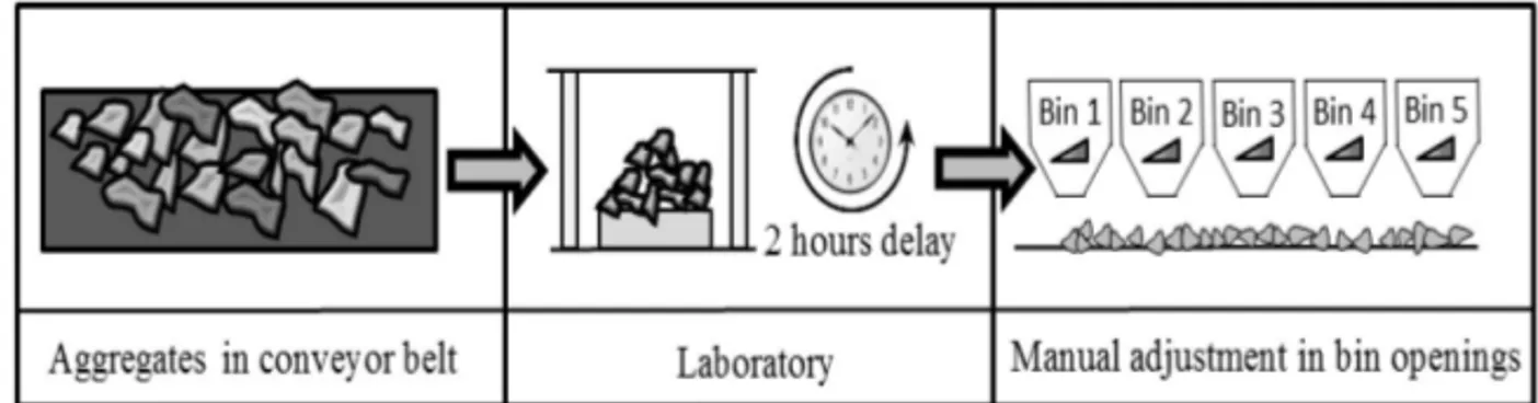
this analysis takes approximately two hours to complete. If the result presents a problem with the product, an operator must take corrective actions. However, this delay generates a product with low quality and several inherent costs. Considering that a typical process of asphalt production has a production rate of 300 tons/hour, this method of offline quality control can generate a waste of about 600 tons of material (Kabadurmus et al., 2010), or this product of poor quality may be used in roads and, in a short time, deteriorates. Figure 1 demonstrates the typical flow of analyses of Hot Mix Asphalt processes.
Figure 1–Typical flow of analyses of Hot Mix Asphalt processes.
In the same way, other processes similar to the one presented in Figure 1 can be found in various industrial plants. Therefore, the improvement solutions for this process can be applied to other similar systems.
3 CONTROL SYSTEM IN REAL TIME
Some authors, such as Kabadurmus et al. (2010) and Zhang et al. (2014), have presented a new method of process control so that the long laboratory analysis time is minimized, and corrective actions are taken faster if necessary. In this approach, analysis techniques by images are applied in the real process. On the conveyor belt, images of the aggregates are taken continuously while an algorithm estimates the gradation of those aggregates.
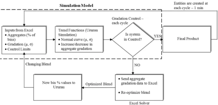
A Discrete Event Simulation (DES) simulates the gradation values of the aggregates in the system used in this work. These values are sent to a spreadsheet (explained in subsequent sections), in which the optimal proportion of the combination of aggregates is calculated. The PLC receives these values and sends input and output signal of bins, as described in to Figure 2. Thus, a process control in real time can be carried out, continuously monitoring the process parameter to be controlled and acting correctively, when necessary, in the actuators that modify the process characteristics.
It can be noticed, in the area highlighted in Figure 2, that a DES software can simulate the values of gradation of those aggregates. The simulation of these values allows running tests in different scenarios giving more flexibility to the system.
Figure 2–Setup of the image analysis control system.
the trend function begins to work. These functions are essential tools for simulation, as they help the computational environment simulate the conditions of the real world. The Normal curve was used in the process, with determined values of mean and pattern deviation.
Figure 3–Integration of physical system with Excel solver.
During the operation, the system continuously verifies if it is under control. We assume a system out of control when the granulation of one of the sieves is out of specification limits of the JMF. As the entities are created, according to the interval of time of discretization, it is also verified if the final product is in the control parameters according to this pre-defined time. The time interval in which the entities are created in this simulation was of 1 minute.
As opening for the optimization system, the current granulation values of each sieve are read from Ururau and written in Excel. After the optimization model reoptimizes the mixture by giving new percentage values to the aggregates, these values are read from Excel and written back to Ururau, and the simulation continues with the new values of the mixture. The simulation continues until it gets the value of ten hours, which means one day of production.
4 INTEGRATION OF SIMULATION MODEL WITH PLC AND EXCEL
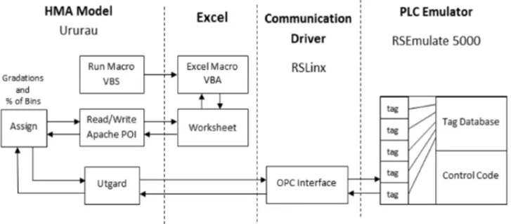
The Ururau software was design to have the capacity to exchange information with PLCs and Excel software. This interaction allows a greater flexibility within the system; it may use the simulation to assist in the testing of other systems. Therefore, Ururau exchanges information with Excel applying the Java API (Application Programming Interface) Apache POI, which operates various file formats based on Office Open XML and Microsoft’s OLE 2 Compound Document format (OLE2) patterns.
Note, in Figure 4, that the Worksheet communicates directly with Ururau software, using “Read/Write” block, which can store Excel information such as internal Ururau variables. This simulation software is also able to run VBA macros in Worksheet. All Information in the Excel can be sent to the PLC by using the Assign block, which applies the OPC Interface to alter the values in Tag Database of PLC.
Figure 4–Integration of simulation model, Ururau, Excel and PLC.
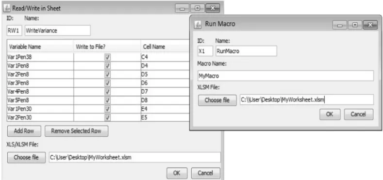
It was also developed a “Read/Write” block and a “Run Macro” block in the development envi-ronment of Ururau so that the user can read and write information in Excel cells and run macros in VBA (Visual Basic for Applications) code. Figure 5 represents these blocks.
Figure 5–Read/Write and Run Macro in Ururau Interface.
the path where the file is in the computer. In the “Run Macro”, the user has to report the name of the macro developed in Excel and the path where the file is located in the computer.
Figure 4 also shows that in order that the VBA macros are run, a parameterized VBS (Visual Basic Script) code file was used, which is executed by Ururau in Java where it opens Excel, runs the desired macro and saves the file keeping the values updated.
The information of the simulation is sent to the PLC using the “Assign” block by the integra-tion of Ururau with the OPC server with the OPC Utgard client. Available at (http:// open-scada.org/projects/utgard). This OPC client is part of the OpenSCADA software; however, it can be used regardless of the platform. The Utgard is 100% pure JAVA OPC Client API and Open Source.
It was used the Rockwell Automation RSEmulate 5000 emulator, which simulates the behavior of a real PLC and communicates with the Ururau by means of its OPC Communication Driver RsLinx.
5 SIMULATION MODEL
The construction of the simulation models followed the methodology proposed by Banks et al. (2010), in which the next steps were taken: formulation of the problem; definition of the ob-jective and overall project plan; elaboration of the conceptual model; data collection; translation of the conceptual model; verification; validation; experimentation; execution and analysis. The verification and validation of the models also followed the steps suggested by Sargent (2013).
process to be tested using different scenarios, enabling adjustments in the control and deep anal-ysis of the process. A Free Open Source Software (FOSS) for the DES called Ururau was used. Full description of the language used in Ururau is available at https://bitbucket.org/ururau/ururau (Peixoto, 2017).
The software was applied to generate the trend curves of the gradation of the aggregates, send information to Excel and communicate with the PLC (Programmable Logic Controller) and with the supervisory system.
The simulation can be followed in real time by the supervisory system developed in the Factory Talk View SE of Rockwell Automation Company, generating graphics in real time and enabling commands, such as Reset of counters. That is illustrated in Figure 6. All simulation parameters are described in Appendix A.
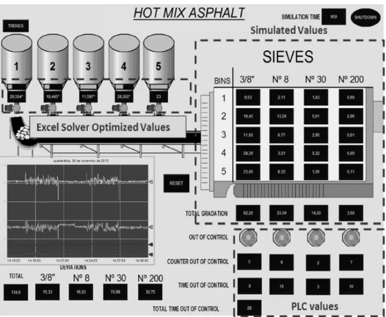
Figure 6–Illustration of Human Machine Interface of Hot Mix Asphalt.
When some sieve is out of control, the signal light “Out of control” will turn red. This indicator is controlled by the PLC with comparison blocks that monitor if the values are within the control parameters. As well as the “Counter out of control” counters (that count the number of times each sieve was out of control), the “Time out of control” (that count the time each sieve was out of control) and “Total Time out of control” (that counts the total time the system was out of control) are monitored in real time by the PLC. This information can be visualized at the bottom right of the Figure. The bar graphs with bin openings of each bin and their respective values are generated by the Solver optimization that calculates the optimal percentage of opening of each bin when the system is out of control and can also be visualized at the top left of the Figure.
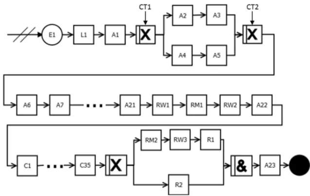
The conceptual model of the system is based on the IDEF-SIM, which is a language used for the conceptual description of a simulation model, presented by Montevechi et al. (2010). Figure 7 represents the conceptual model used to simulate the Hot Mix Asphalt Production.
Figure 7–Conceptual model in IDEF-SIM.
The element E1 (Create) creates entities every 1 minute in the simulation. The elements L1 (Hold), A1 (Assign) and A23 (Assign) form a set, in which the next entity created by the element E1 is only released after the previous entity has passed by all elements of the simulation. That is, the entities pass through the simulation elements, one at a time. The structure of OR, A2, A3, A4 and A5 (Assigns) is used to generate a trend function that describes a possible change in aggregate gradation over time. The trend function applied in the work is the alternating step function, according to Figure 8.
Figure 8–Alternating step Function.
calculations of the Excel, and then the RW2 will read the updated and calculated values of the spreadsheet.
The A22 has the function of totalizing the sieves deviation. Structure C1 up to C35 has the function of communicating all needed values with the PLC. The OR, RM2, RW3, R1, and R2 structure has the function of verifying whether there is any sieve out of control. If there is one or more out of control, then the RM2 will activate the Solver that will calculate the proportions of Bin openings to optimize the mixture. These values are read from Excel by the element RW3, and the R1 will count how many times the mixture was optimized. The R2 element counts how many times the mixture was under control and optimization was not necessary.
6 INPUT DATA AND PARAMETERS
At the same time, the model works with a spreadsheet in a MS Excel file. In this file, there are the inputs of the simulation models. Zhang (2014) reported that The U.S. National Center for Asphalt Technology provides the input data for testing the system. These data are commonly observed in operations of asphalt plants and specifications and limits of typical mixture projects.
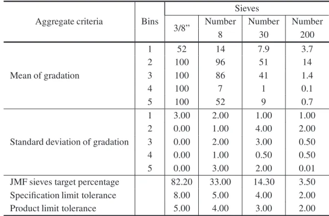
Table 1–The Aggregate Input Data and Specifications (Zhang, 2014).
Aggregate criteria Bins
Sieves
3/8” Number Number Number
8 30 200
Mean of gradation
1 52 14 7.9 3.7
2 100 96 51 14
3 100 86 41 1.4
4 100 7 1 0.1
5 100 52 9 0.7
Standard deviation of gradation
1 3.00 2.00 1.00 1.00 2 0.00 1.00 4.00 2.00 3 0.00 2.00 3.00 0.50 4 0.00 1.00 0.50 0.50 5 0.00 3.00 2.00 0.01 JMF sieves target percentage 82.20 33.00 14.30 3.50 Specification limit tolerance 8.00 5.00 4.00 2.00 Product limit tolerance 5.00 4.00 3.00 2.00
The initial percentages of the Mixing Project and the upper and lower limits of the five silos of cold inputs are demonstrated in Table 2. The percentage of each silo during the production has to be within its upper and lower limits, and this restricts the procedure of process optimization.
Table 2–The Aggregate Initial Data and Limits (Zhang, 2014).
Bin Initial proportion Bin capacity range percentage Minimum Maximum
1 37 17 57
2 14 5 23
3 7 2 12
4 30 10 50
5 12 5 23
7 OPTIMIZATION MODEL
All the restrictions of the process depend on the JMF required. The optimization algorithm was adapted from Kabadurmus et al. (2010) and is defined as follows:
min
j Dj =
|nj −ixigi j|
rmaxj −rminj 2 (1)
s.t.: smaxi ≤xi =simin (2)
rmaxj ≤ i
xigi j ≤rminj (3)
i
xi =1 (4)
xi ≥0 (5)
whereiis each cold feed bins, jis each sieves, D jis the total deviation.
The decision variable of the model is:
• Weight percentage of the total mixture from the bins(xi).
The parameters are:
• Gradation measurements from bins(gi j);
• Target levels (by JMF) for % passing the sieves(nj);
• Upper and lower limit of specification % of passing through the sieves(rmaxj ,rminj );
• Upper and lower limit for % of weigh coming from each silo(simax,simin).
8 COMPUTATIONAL EXPERIENCE AND RESULTS
The simulation was tested in various scenarios, combining variations in input gradation and specification limits, comparing the process efficiency without the Solver and with the Solver optimization. The control limits applied are the Specification Limit Tolerance and Product Limit Tolerance, described in Table 1. When the product was out of these limits, they were considered out of control. Two cases for the variations in the input gradation were employed: Low Variation (described in Table 1) and High Variation (the values of Table 1 multiplied by 1.5). The results were obtained by a single simulation round equivalent to 10 hours (600 minutes) simulated, corresponding to one working day in a typical HMA production plant.
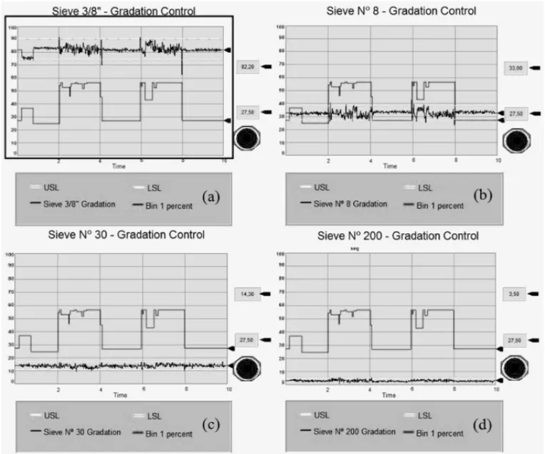
The results are in the HMI software generating graphics and showing the immediate values of the variables according to Figure 9.
Figure 9–Screen shot of simulation output for low variation solver control strategy: (a) gradation of sieve 3/8” from all bins (top) with bin 1 percentage of the mix (bottom); (b) gradation of sieve #8 from all bins with bin 1 percentage of the mix; (c) gradation of sieve #30 from all bins (bottom) with bin 1 percentage of the mix (top); (d) gradation of sieve #200 from all bins (bottom) with bin 1 percentage of the mix (top).
It can also be seen the results by the report generated by the Ururau software that, at the end of the simulation round, creates a detailed report of the simulation and its variables. An example of a part of this report is in Figure 10.
User Variables mean standard half-width minimum maximum deviation
GradSieve38 82.370 NaN NaN 82.370 82.370
GradSieve8 34.330 NaN NaN 34.330 34.330
GradSieve30 13.156 NaN NaN 13.156 13.156
GradSieve200 3.249 NaN NaN 3.249 3.249
TotalcumDeviation 572.056 NaN NaN 572.056 572.056
Counters mean standard half-width minimum maximum
deviation
R1 CounterSolver 25.000 NaN NaN 25.000 25.000
R2 CounterOK 576.000 NaN NaN 576.000 576.000
Figure 10–Part of the report generated by Ururau.
The results are summarized in Table 3.
Table 3–Results of Simulations.
Control Strategy % Reduction
Control Aggregate No Solver Time Total Limit Variation Control Control Out of Cumulative
Control Deviation
SL Low 31 (0) 25 (25) 19.35 28.93 804.86 572.05
SL High 70 (0) 63 (67) 10.00 22.06 944.22 735.95
PL Low 544 (0) 40 (39) 92.65 38.55 1156.73 710.81
PL High 502 (0) 139(140) 72.31 28.83 1313.23 934.62
*#time out of limits (#mix changes). Total cumulative deviation from all sieves.
Note: SL (Specification Limit); PL (Product Limit).
According to Table 3, the optimization obtained a better result with the Production Limit Toler-ance, which is more limited than the Specification Limit TolerToler-ance, presenting an improvement of 92.65% in the time out of control when compared to No Control System Strategy. However, the optimization did not prove to be effective when the system presented a high variation in its input aggregates, in comparison with the system that has a lower variation, activating the solver more frequently and generating instabilities in the system.
9 CONCLUDING REMARKS
This work describes a real time on-line control of dosing input aggregates for hot mix asphalt production. The free and open source discrete event simulation software Ururau was applied to simulate the process, exchange data and manipulate spreadsheets in the Excel software. The Solver was used to optimize the mixture in real time. One of the main difficulties in the dosing processes is the variety in its inputs and the capacity of rapidly identifying and correcting this deviation. The system presented proved to be effective in this correction during the production, guaranteeing a standardization and an increase of quality in the final product.
The application for hot mix asphalt process proved itself efficient; however, this principle may also be applied to other input dosing processes. Knowing the variables, curves, and restrictions of the processes, this system shows flexibility and safety as it allows logic tests, commissioning and adjustments in the control system, with no damage to the real system, besides the code of the Ururau software is open, enabling the user to adapt the software to his/her preference and carry out a series of tests.
The aim of this new simulation software is to disseminate, use and understand discrete event simulation in Brazil, allowing the users to be in contact with this specific software for simulation, developing his/her abilities and having the possibility to know the internal conception of the software structure.
ACKNOWLEDGMENTS
The authors thank the Coordination for the Improvement of Higher Education Personnel (CAPES), the National Council for Scientific and Technological Development (CNPq) and the Research Foundation of the State of Rio de Janeiro (FAPERJ) for financial support for this re-search. Thanks are also due to Maria Marta Garcia for assistance in translating the paper.
REFERENCES
[1] BANKSJ, CARSONSJ, NELSONBL & NICOLD. 2010. Discrete-event system simulation, (5 ed.). New York: Prentice Hall: Englewood Cliffs. 622 p.
[2] CHRISTENSEND. 2010. A mix design manual for Hot Mix Asphalt – Draft Report, National Co-operative Highway Research Program (NCHRP), National Academy of Sciences, Washington, D.C. Conference, 1522–1533.
[3] FUMC, ANDRADOTTIRS, CARSONJS, GLOVERF, HARRELLCR, HOY, KELLYJP & ROBIN
-SONSM. 2000. Integrating optimization and simulation: Research and practice. In:Winter Simulation Conference Proceedings,1: 610–616.
[4] IMOLEOI, KRIJGSMAND, WEINHARTT, MAGNANIMOV, CHAVEZ´ MONTESBE, RAMAIOLIM & LUDINGS. 2016. Experiments and discrete element simulation of the dosing of cohesive powders in a simplified geometry. In:Powder Technology,287: 108–120.
[5] JAHANGIRIANM, ELDABIT, NASEERA, STERGIOULASLK & YOUNGT. 2010. Simulation in manufacturing and business: A review.European Journal of Operational Research,203(1): 1–13. [6] KABADURMUSO, PATHAKO, SMITH JS, SMITHAE & YAPICIOGLU H. 2010. A simulation
[7] MONTEVECHIJAB, LEALA, PINHOA, COSTARF, OLIVEIRAML & SILVAAL. 2010. Concep-tual modeling in simulation projects by mean adapted IDEF: An application in a Brazilian Company. In: Proceedings of the Winter Simulation Conference, edited by JOHANSSONB, JAINS, MONTOY
-ATORRESJ, HUGANJ & Y ¨UCESANE, 1624–1635. Piscataway, New Jersey: Institute of Electrical and Electronics Engineers, Inc.
[8] OESTERREICHTD & TEUTEBERGF. 2016. Understanding the implications of digitisation and au-tomation in the context of Industry 4.0: A triangulation approach and elements of a research agenda for the construction industry. In:Computers in Industry,83: 121–139.
[9] PEIXOTO TA, RANGEL JJA, MATIAS IO, SILVA FF & TAVARES ER. 2017. Ururau: a free and open-source discrete event simulation software. Journal of Simulation, 11: 303–321. [doi.org/10.1057/s41273-016-0038-5].
[10] SARGENTRG. 2013. Verification and validation of simulation models.Journal of Simulation,7(1): 12–24.
[11] SCHUHG, REUTERC, HAUPTVOGELA & D ¨OLLEC. 2015. Hypotheses for a Theory of Produc-tion in the Context of Industry 4.0. In: Advances in ProducProduc-tion Technology. Springer InternaProduc-tional Publishing. Lecture Notes in Production Engineering, p. 11–23. [DOI 10.1007/978-3-319-12304-2 2]
[12] XUJ, HUANGE, HSIEHL, LEELH, JIAQ & CHENC. 2016. Simulation optimization in the era of Industrial 4.0 and the Industrial Internet. In: Int. J. Simulation and Process Modelling, 10(4): 310–320.
[13] ZHANGM, HEITZMANM & SMITHAE. 2014. Improving hot mix asphalt production using com-puter simulation and real time optimization.J. Comput. Civ. Eng., 2014.28. In: American Society of Civil Engineers (ASCE), p. 1–7 [DOI: 10.1061/(ASCE)CP.1943-5487.0000302].
Appendix A– Simulation parameters.
Name Function Parameters E1 Create Constant (1)min L1 Hold if Release == 0
CT1 OR (TNOW<=120)((TNOW>240) && (TNOW<=360))(TNOW>480) A1 Assign (Variable) Release == 1
A2 Assign (Variable) Function1 == 1.33 A3 Assign (Variable) Function2 == 0.67 A4 Assign (Variable) Function1 == 0.67 A5 Assign (Variable) Function2 == 1.33 CT2 OR 100% (Union)
Appendix A– (continuation).
Name Function Parameters
A11 Assign (Variable) Var5Sieve8 == Function2*NORM(52,3) A12 Assign (Variable) Var1Sieve30 == Function2*NORM(7.9,1) A13 Assign (Variable) Var2Sieve30 == Function1*NORM(51,4) A14 Assign (Variable) Var3Sieve30 == Function2*NORM(41,3) A15 Assign (Variable) Var4Sieve30 == Function1*NORM(1,0.5) A16 Assign (Variable) Var5Sieve30 == Function2*NORM(9,2) A17 Assign (Variable) Var1Sieve200 == Function2*NORM(3.7,1) A18 Assign (Variable) Var2Sieve200 == Function1*NORM(14,2) A19 Assign (Variable) Var3Sieve200 == Function2*NORM(1.4,0.5) A20 Assign (Variable) Var4Sieve200 == Function1*NORM(0.1,0.05) A21 Assign (Variable) Var5Sieve200 == Function2*NORM(0.7,0.01) RW1 Read/Write in Excel Write all sieves functions in Excel
RM1 Run Macro in Excel VBA “Application.CalculateFull” RW2 Read/Write in Excel Read Sieves Gradation, Deviations,
# Sieve Out Specifications, % Bin Openings A22 Assign (Variable) AcumDeviation == AcumDeviation + TotalDeviation
Appendix A– (continuation).
Name Function Parameters C21 Communication (Real Tag) Bin1Sieve30 C22 Communication (Real Tag) Bin2Sieve30 C23 Communication (Real Tag) Bin3Sieve30 C24 Communication (Real Tag) Bin4Sieve30 C25 Communication (Real Tag) Bin5Sieve30 C26 Communication (Real Tag) GradationSieve30 C27 Communication (Real Tag) DeviationSieve30 C28 Communication (Real Tag) Bin1Sieve200 C29 Communication (Real Tag) Bin2Sieve200 C30 Communication (Real Tag) Bin3Sieve200 C31 Communication (Real Tag) Bin4Sieve200 C32 Communication (Real Tag) Bin5Sieve200 C33 Communication (Real Tag) GradationSieve200 C34 Communication (Real Tag) DeviationSieve200 C35 Communication (Real Tag) TotalDeviation
OR2 OR # Sieve Out Specifications>= 1 RM2 Run Macro in Excel VBA “SolverSolve(True)” RW3 Read/Write in Excel Read Sieves Gradation, Deviations,