SPATIO-TEMPORAL PREDICTION OF ELECTRIC POWER SYSTEMS INCLUDING EMERGENT RENEWABLE ENERGY SOURCES JAYME MILANEZI JUNIOR

(1)

UNIVERSIDADE DE BRAS´ILIA FACULDADE DE TECNOLOGIA

DEPARTAMENTO DE ENGENHARIA EL´ETRICA

SPATIO-TEMPORAL PREDICTION OF ELECTRIC

POWER SYSTEMS INCLUDING EMERGENT

RENEWABLE ENERGY SOURCES

JAYME MILANEZI JUNIOR

ORIENTADOR: JO ÃO PAULO CARVALHO LUSTOSA DA COSTA COORIENTADOR: JOSÉ ANT ÔNIO ALVES GOMES

DISSERTAÇ ÃO DE MESTRADO EM ENGENHARIA ELÉTRICA

PUBLICAC¸ ˜AO: 554/2014 DM PPGEE

(2)

(3)

UNIVERSIDADE DE BRAS´ILIA FACULDADE DE TECNOLOGIA

DEPARTAMENTO DE ENGENHARIA EL´ETRICA

SPATIO-TEMPORAL PREDICTION OF ELECTRIC

POWER SYSTEMS INCLUDING EMERGENT

RENEWABLE ENERGY SOURCES

JAYME MILANEZI JUNIOR

DISSERTAC¸ ˜AO DE MESTRADO SUBMETIDA AO DEPARTAMENTO

DE ENGENHARIA EL´ETRICA DA FACULDADE DE TECNOLOGIA

DA UNIVERSIDADE DE BRASÍLIA, COMO PARTE DOS REQUISITOS NECESS ÁRIOS PARA A OBTENÇ ÃO DO GRAU DE MESTRE EM EN-GENHARIA ELÉTRICA.

APROVADA POR:

Prof. Jo˜ao Paulo C. Lustosa da Costa, Dr.-Ing. (ENE-UnB) (Orientador)

Prof. Jos´e Antˆonio Alves Gomes, Dr. (INPA) (Coorientador)

Prof. Ricardo Zelenovsky, Dr. (ENE-UnB) (Examinador Interno)

F´abio Stacke Silva, Dr. (ANEEL) (Examinador Externo)

(4)

FICHA CATALOGR ´AFICA MILANEZI JR, JAYME

FOLHA CATALOGR ´AFICA - Spatio-Temporal Prediction of Electric Power Systems including Emergent Renewable Energy Sources.

[Distrito Federal] 2014. xxviii, 146p., 297mm (ENE/FT/UnB, Mestre, Engenharia El´etrica, 2014).

Disserta¸c˜ao de Mestrado - Universidade de Bras´ılia. Faculdade de Tecnologia.

Departamento de Engenharia El´etrica.

1. Predi¸cão de Séries Temporais 2. Sistemas de Potência 3. Fontes Alternativas de Energia 4. Processamento de Sinais

I. ENE/FT/UnB II. Publica¸c˜ao 554/2014 DM PPGEE

REFERˆENCIA BIBLIOGR ´AFICA

MILANEZI JR., J. (2014). Spatio-temporal Prediction of Electric Power Systems in-cluding Emergent Renewable Energy Sources. Disserta¸cão de Mestrado em Engenharia Elétrica, Publica¸cão 554/2014 DM PPGEE, Departamento de Engenharia Elétrica, Universidade de Bras´ılia, Bras´ılia, DF, 146p.

CESS ˜AO DE DIREITOS

NOME DO AUTOR: Jayme Milanezi Junior.

TÍTULO DA DISSERTAÇ ÃO DE MESTRADO: Spatio-temporal Prediction of Elec-tric Power Systems including Emergent Renewable Energy Sources.

GRAU / ANO: Mestre / 2014

O autor permite, desde já, a reprodu¸cão total ou parcial desta disserta¸cão de mestrado, desde que seja rigorosamente respeitada a cita¸cão da fonte.

Jayme Milanezi Junior SQN 409, bloco I,

(5)

Não posso imaginar que uma vida sem trabalho seja capaz de trazer qual-quer espécie de conforto. A imagina¸cão criadora e o trabalho, para mim, andam de mãos dadas; não retiro prazer de nenhuma outra coisa.

(6)

DEDICAT ´

ORIA

`

(7)

AGRADECIMENTOS

`

A minha esposa, Maria Galberianny, que, com amor, companheirismo e verdadeira doa¸cão, tolerou meu frequente distanciamento em virtude dos numerosos trabalhos que empreendi durante este mestrado. A você, que sempre confiou na minha capacidade, me apoiando e fortalecendo a minha moral para este bom combate, agrade¸co de todo o meu cora¸cão. Amo você.

Agrade¸co ao meu orientador e ex-colega de profissão, Prof. João Paulo, com cuja amizade conto desde os tempos em que ombreamos no Instituto Militar de Engenharia (IME). Enquanto Professor, sempre me dispensou inestimável ajuda no âmbito do mestrado, tendo me apresentado um insti-gante e desafiador campo de pesquisa, e dirimindo várias de minhas dúvidas em tempo real. Pelo exemplo e incentivo incansáveis, sou-lhe extremamente grato.

Aos meus colegas na Agência Nacional de Energia Elétrica (ANEEL), prin-cipalmente aos meus companheiros na Superintendência de Pesquisa e De-senvolvimento e Eficiência Energética (SPE), por terem prestigiado os meus esfor¸cos ao longo da prepara¸cão desta disserta¸cão. Ao Superintendente, Máximo Luiz Pompermayer, agrade¸co pela confian¸ca em que o meu trabalho na SPE prosseguiria sem maiores percal¸cos, mesmo com o desenvolvimento concomitante das tarefas relacionadas ao mestrado. Igualmente, gostaria aqui de deixar meus agradecimentos a Aurélio Calheiros Melo Junior, As-sessor da SPE, por ter sempre demonstrado apoio e incentivo às tarefas acadêmicas, e aos demais colegas de sala e de toda a ANEEL, que foram grandes amigos, verdadeiros vetores de renova¸cão e bom humor ao longo desta jornada. Um especial agradecimento a Lucas Dantas Xavier Ribeiro, que veio a se tornar um fundamental colaborador em alguns tópicos da pre-sente disserta¸cão, auxiliando-me com algumas sintaxes de MATLAB e na organiza¸cão e processamento de dados em sua distribui¸cão espacial. Muito obrigado a todos vocês.

(8)

`

A pesquisadora Renata Schmidt, da Universidade Federal do Amazonas (UFAM), pela colabora¸cão dada juntamente com o Prof. José Gomes, e ao Prof. José Luiz Cerda-Arias, que nos forneceu os dados de 29 subesta¸cões elétricas da cidade de Leipzig - Saxônia, Alemanha, também dedico meu sincero reconhecimento. Deixo aqui também um obrigado a Ronaldo Se-bastião Ferreira Junior, que me prestou grande aux´ılio na concep¸cão de alguns circuitos para a parte de reciclagem de ondas rádio e na própria parte de reciclagem de luz indoor.

Aos meus colegas em inova¸cões tecnológicas e matérias de mestrado Marco Antônio Marques Marinho, Edison Pignaton, Antonio Rubio Serrano, Danilo Fernandes, Bruno Pilon, Ricardo Kehrle e Stephanie Alvarez, agrade¸co pela parceria, seja nos estudos em conjunto, seja naqueles debates teóricos sobre os modelos estudados, cujas discussões sempre foram da maior relevância, sempre por demais construtivas. Ao Prof. Ricardo Zelenovsky e a Fábio Stacke Silva, integrantes da banca avaliadora, sou grato pelas valorosas re-visões do texto final desta disserta¸cão, as quais tornaram o texto de leitura sem dúvida mais apraz´ıvel.

Aos meus pais, Jayme e Lúcia, que, com amor e paciência, me deram desde cedo o ensinamento de que o estudo, a honestidade e a supera¸cão pessoal moldam os únicos caminhos que edificam e valorizam permanentemente nossas vidas. Aos meus irmãos Pollyanna, Marcos e Thiago, pelo suporte emocional e conversas revigorantes. Vocês são um grande esteio de carinho e amparo na minha vida.

Agrade¸co, por fim...

(9)

RESUMO

PREDIÇ ÃO ESPACIAL TEMPORAL DE SISTEMAS ELÉTRICOS DE POTÊNCIA INCLUINDO FONTES RENOV ÁVEIS EMERGENTES Autor: Jayme Milanezi Junior

Orientador: João Paulo Carvalho Lustosa da Costa Coorientador: José Antônio Alves Gomes

Programa de Pós-gradua¸cão em Engenharia Elétrica Bras´ılia, mar¸co de 2014

A atividade de planejamento de sistemas de potência inclui, como um de seus maiores desafios, a predi¸cão do comportamento da carga. Com a finalidade de otimizar o investimento ante os dados de consumo, as empresas do setor elétrico lan¸cam mão de várias técnicas de previsão da evolu¸cão da demanda que devem atender. No presente trabalho, o tema da predi¸cão espacial e temporal da carga é enfrentado, estudando e incorporando, simultaneamente, a tendência hoje já observada de inclusão de fontes em microgera¸cão distribu´ıda. Três fontes renováveis e emergentes de gera¸cão foram consideradas como geradoras de energia pelos consumidores: enguias elétricas, painéis fotovoltaicos para aproveitamento da luz solar e de interiores, e antenas para reciclagem da energia existente nas ondas eletromagnéticas de radiodifusão. Quatro métodos preditivos foram empregados para prever o comportamento da carga: modelo Auto-Regressivo (AR), Auto-Auto-Regressivo com Variável eXógena (ARX), Auto-Auto-Regressivo de Média Móvel com Variável eXógena (ARMAX) e Redes Neurais Artificiais (ANN). Os dados de consumo foram as máximas demandas semanais registradas em 8 Subesta¸cões da cidade de Leipzig (Saxônia, Alemanha), durante os anos de 2001, 2002, 2003 e 2004. O dado exógeno considerado foi a temperatura, em valores diretos e logar´ıtmicos. Das 209 semanas existentes entre 2001 e 2004, as 200 primeiras destinaram-se ao ajuste dos coeficientes nos modelos AR e ao treinamento da rede neural; as 9 semanas restantes foram destinadas à compara¸cão de resultados. A aplica¸cão das técnicas deu-se, assim, em dois estágios: no primeiro, os dados reais da rede de Leipzig foram considerados, e no segundo estágio trabalhou-se com novos valores de demandas máximas, originadas pela inser¸cão de valores hipotéticos de energia recebida das três fontes citadas. Em ambos os estágios, o modelo ARMAX foi o de melhor precisão na previsão de dados. O sistema de redes neurais demonstrou ser um sistema sub-ótimo de previsão.

(10)

ABSTRACT

SPATIO-TEMPORAL PREDICTION OF ELECTRIC POWER SYSTEMS INCLUDING EMERGENT RENEWABLE ENERGY SOURCES

Author: Jayme Milanezi Junior

Supervisor: João Paulo Carvalho Lustosa da Costa Co-supervisor: José Antônio Alves Gomes

Programa de Pós-gradua¸cão em Engenharia Elétrica Bras´ılia, March of 2014

Power systems planning activities include load behavior prediction as one of its most challenging tasks. In order to optmize investments related to consumption data, util-ities from the Electrical Sector resort to several forecasting techniques so that they can predict the power demand which these utilities must support. Along the present work, issues related to the spatial and temporal predictions are faced, considering, simultaneously, the observed trend of microgeneration spread. Three emergent renew-able sources were proposed to be taken on by consumers: electric eels, photovoltaic solar panels for outdoor generation and indoor light energy harvesting, and antennas for radio frequency energy recycling. Four predictive methods were employed in order to forecast load evolution: Auto-Regressive (AR), Auto-Regressive with eXogeneous inputs (ARX), Auto-Regressive Moving Average with eXogeneous inputs (ARMAX) models and Artificial Neural Networks (ANN). Consumption data were the maximum weekly power demands registered over 8 Power Substations from the city of Leipzig (Saxony, Germany), during the years 2001, 2002, 2003 and 2004. The exogeneous variable adopted was temperature, in realistic and in logarithmic values. During the 209 weeks which are comprised between 2001 and 2004, the first 200 weeks served to coefficients adjustments, with regards to AR models, and the trainning of the neural network, in the case of ANN. The last 9 weeks were destinated for results compari-son. Techniques were undertaken in two stages: firstly, only realistic data from Leipzig Substations were considered, and in the second stage, new values for maximum power demands were obtained by means of simulations upon the three emergent sources. In both stages, ARMAX model returned the fittest results, whereas ANN characterized itself as a sub-optimal prediction system.

(11)

(12)

List of Tables

1.1 Oferta Interna de Energia (OIE), Produto Interno Bruto (PIB) e Pop-ula¸c˜ao, de 2003 a 2012, no Brasil [4] . . . 2 2.1 Domestric Energy Supply (DES), Gross Domestic Product (GDP) and

Population from 2003 to 2012 in Brazil [4] . . . 2 3.1 Frequency bands of energy harvesting and respective maximum dBm

power . . . 13 3.2 Incident power as a function of dBm values - examples . . . 19 3.3 Maximal Efficiency Values for Crystalline Silicon, Amorphous Silicon,

and Organic BHJ Solar Cells under different spectral illumination [24]. 20 3.4 Annual Average of Daily Irradiance [Wh/m2_{] by Brazilian Region [40].} ₃₁

3.5 Summary about three energetic sources: RF harvesters, indoor light recycling, electric eels. . . 43 4.1 AR and ARX models performances in terms of prediction focus and

FPE, considering temperature and log temperature as eXogeneous vari-ables in ARX cases. . . 50 4.2 Mean Square Errors (MSE) and Number of Positive Deviations (NPD)

for AR, ARX, ARX log[T] and ARMAX log[T], na = 10, nb = 10 and

nk = 1 . . . 52

5.1 MSE for AR, ARX, ARX log[T], ARMAX and ANN, and the best num-ber of hidden layers for ANN system in function of each combination of w, a and k, for periods of 35 and 50 weeks. . . 71 5.2 MSE for AR, ARX, ARX log[T], ARMAX and ANN, and the best

num-ber of hidden layers for ANN system in function of each combination of w, a and k, for periods of 65 and 80 weeks. . . 72 5.3 MSE for AR, ARX, ARX log[T], ARMAX and ANN, and the best

(16)

5.4 MSE for AR, ARX, ARX log[T], ARMAX and ANN, and the best num-ber of hidden layers for ANN system in function of each combination of w, a and k, for periods of 135 and 150 weeks. . . 75 5.5 Number of cases in which a model achieves the best approximation,

(17)

List of Figures

1.1 Esquema reduzido do sistema elétrico, compreendendo geradores hidrelétricos distantes, longas linhas de transmissão, distribui¸cão e consumo . . . 4 1.2 Esquema da Fig. 1.1, agora incluindo enguias elétricas nadando em um

rio e recicladores RF sobre as casas, ambos fornecendo energia para o sistema elétrico interligado, enquanto um analisador de dados reúne os dados de consumo das Subesta¸cões envolvidas . . . 5 1.3 Compara¸cão entre as redes com e sem microgeradores distribu´ıdos: a

pessoa representa os geradores, a corda é comparada com as linhas de transmissão, um bloco pesado representa a carga, e o contrapeso auxiliar representa a microgera¸cão: (a) a pessoa efetua o esfor¸co sozinha, e (b) o esfor¸co de sustentar a carga é parcialmente dividido entre ela e o contrapeso auxiliar. . . 5 2.1 Reduced scheme of the electric system, comprehending far away

hydro-generators, long transmission lines, distribution and consumption. . . . 4 2.2 Scheme of Fig. 1.1, now including eels into the river and an RF recycler

on top of houses, both delivering generating power for the interconnected power system, while a data analyzer gathers up the consumption data from the Power Substations. . . 5 2.3 Comparison of the grid with micro-generators: the man represents

gen-erators, the rope is compared to transmission lines, a heavy block repre-sents the load, and the auxiliary counterweight stands for the renewable sources: (a) the man pulls it alone, and (b) the burden of load is partially shared between him and the auxiliary weight. . . 5 3.1 Components of a RF energy harvesting system: the rectenna is an

an-tenna with a RF-DC interface [5]. Therefore, the receiver must be inte-grated to a matching circuit, a voltage booster and the rectifier, whose output is often connected to a battery. . . 11 3.2 Resulting Vout according to input dBm [6]. . . 14

(18)

3.4 Map of Brasilia-DF (Brazil) with the indicated 4 places on which RF spectrum intensities were measured. . . 16 3.5 Measurements of incident dBm power according to frequency. Each

place encloses morning, afternoon and evening data, which are mixed in each graph. . . 17 3.6 Results which overcome -15 dBm, here called “best results”, with values

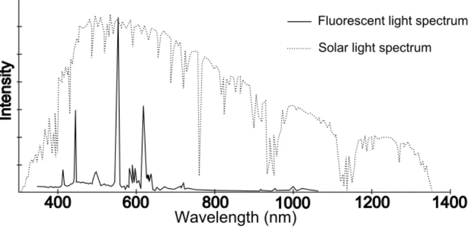
properly signalized in order to show participation of each place in this group. . . 18 3.7 Typical solar light AM 1.5 and cold-cathode fluorescent light spectra. . 21 3.8 Absorbed Light Intensity Lx [lux] versus Open Circuit Voltage Voc [V]

of the solar panel 95 mm x 110 mm for a LED 8 W lamp. . . 22 3.9 Absorbed Light Intensity Lx [lux] versus Short Circuit CurrentIsc[mA]

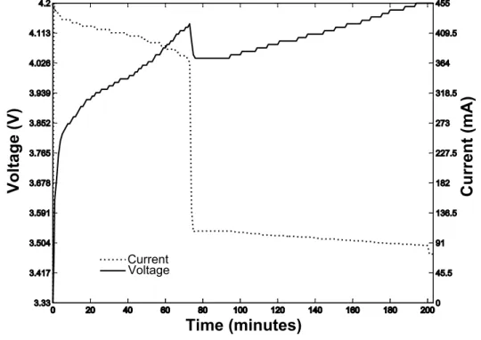
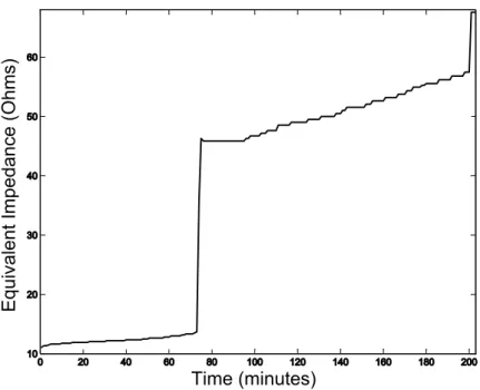
of a solar panel 95 mm x 110 mm for a LED 8 W lamp. . . 22 3.10 Current and voltage versus time of a cell phone charging at 220 V, 60 Hz. 23 3.11 Apparent Impedance (Ω) of cell phone seen by the source. . . 25 3.12 Instantaneous transferred power to the cell phone as seen by the source. 25 3.13 Overall deployment of cell phone, amperimeter (in series) and solar panel

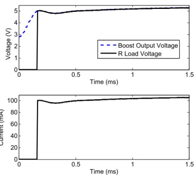
under a light-support in an office for electrical current measurement. . . 26 3.14 Designed boost converter producing 5 V in steady state . . . 27 3.15 Effective voltage and current in steady state over a load of resistive load

R of 50 Ω. . . 29 3.16 Bars indicating equal periods of time A and B as demonstration that

transferred power is influenced by resistance (PB>PA). . . 29 3.17 Electrocytes behavior which yields an external electric voltage: (a) cell

membrane is permeable only to K+ _{ions; (b) Acetylcholine activates the}

electrocyte cell, making Na+ _{ions to come inside it [43]. In the case}

of Electrophorus electricus, there exists only the posterior membrane, which is excitable. . . 33 3.18 Lines of electric field generated along the eel’s body. The head is the

positive pole, and the tail bears the negative pole, from where electric current goes off through water until the head [44]. . . 34 3.19 Equivalent circuit of the electric eel [45]. . . 34 3.20 Real experiment carried out in LFCE-INPA, wherein the electrodes are

(19)

3.21 Picture which outlines the overall deployment of the experiment: two metal plaques actuating as electrodes were placed on each side of the largest width, which is 120 cm. Two resistances were then purposefully inserted in the part of circuit the voltimeter was connected. . . 36 3.22 Equivalent circuit of Fig. 3.21, illustrating the eel as the voltage source.

Ra is the varying water resistance, and 8 Ω corresponds to the total

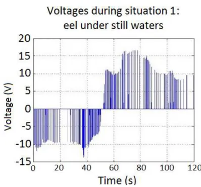
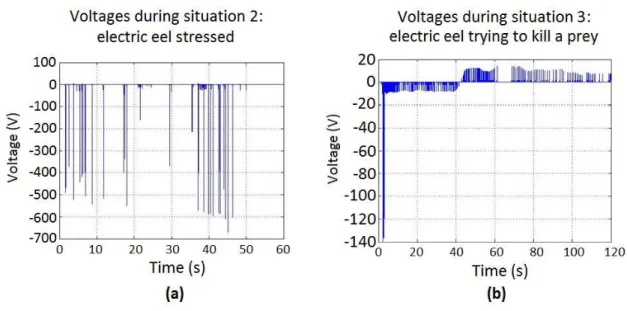
electrodes resistances in series. The resistances of 3 Ω were inserted to protect the voltimeter and to improve measuring accuracy. . . 36 3.23 Voltage values with the eel swimming freely into the aquarium. . . 37 3.24 Voltage values with (a) the eel being stressed, and (b) eel trying to kill

a little prey that is placed in the aquarium. . . 39 3.25 Perspective view of the basket, or aquarium-corral. The brown lines

represent conductors, either nude cable or bars, each one being connected to a different polarity of the external circuit of power management. . . 40 3.26 Upper views of the basket: (a) view of the basket without eels inside;

(b) view of the basket with one eel swimming inside the corral. At any moment of the displacement of the eel, both head and tail are likely to be near to the collecting current points, which are the conductive cables. 41 3.27 Proposed scheme for energy harvesting from eels in a river, which

com-prises eels inside the baskets. All the output cables are connected to a power manager circuit, which carries out this power to be conditioned. 42 4.1 Visual representation of the set of values which influences the next

fore-casted output y(t) at each moment: underlining (a) values which in-fluence output y(k+ 5) and, and in the next instant, (b) values which influence y(k+ 6). . . 45 4.2 Maximum electric power demands over the 209 weeks: letters on the top

indicate the PS. Yellow bar on H substation graph shows the forecasted period for every PS. . . 47 4.3 Models which have provided the minor deviation absolute values, for

each week and PS. . . 52 4.4 Absolute deviation values from Fig. 4.2 divided by the respective

mea-sured values, in percentages . . . 53 4.5 Score of minor deviation absolute values, matching ARX log[T] versus

ANN, for each week and PS . . . 54 4.6 Score of minor deviation absolute values, from the match ARMAX log[T]

(20)

4.7 Measured data and forecast data for Power Substation D (3092), during the 9 last weeks of 2004. . . 55 4.8 Measured data and forecast data for Power Substations A, B, C, E, F,

G and H during the 9 last weeks of 2004. . . 56 4.9 ARMAX forecasted maximum electric power demands for 2005 and

2006, for every PS: the blue line relates to measured data, whereas red lines describe ARMAX prediction data. . . 58 4.10 Leipzig Map with the 8 Power Stations located [52]. . . 59 5.1 Example of electric demand series: d1 is the overall demand from

con-sumers, d2 is the energy the PS furnishes, and Pµg is the power

micro-generation, so that Pµg =d1−d2. . . 61

5.2 (a) Increasing annual data for cell phones in Brazil since 1990; (b) In-creasing annual data for cable TV in Brazil since 1993 (Anatel). . . 62 5.3 Two curves expressing temporal evolution parameters for different sources. 63 5.4 Evolution of grid-connected and off-grid PV panels, in MW (IEA PVPS),

in Japan. . . 64 5.5 Diagram for the routine by which unilateral white noise k is inserted

into original exponential series. . . 67 5.6 Global rate over two years, firstly considering pure exponential e0.025t

evolution (a), and then handling values with oscillation upon e0.025t _(b).

These last values are believed to be more probable into the market en-vironment. . . 67 5.7 Weekly actual values of square meter PV panels and RF antennas for

the initial value of 50 m2 _{in the considered PS. . . .} ₆₈

5.8 New version for Fig. 4.6, now adopting w = 104, a = 2.0, k = 2.5 and c= 50. Realistic Data corresponds to Measured Data from Fig. 4.6. . . 77 5.9 New version for Fig. 4.6, now adopting w = 104, a = 2.0, k = 2.5 and

c= 50. Realistic data corresponds to measured data from Fig. 4.7. . . 78 5.10 Curves of demand with no sources generating, with the three sources

and with only eels and RF antennas. . . 78 5.11 Antennas generating from January 2002, initial quantity of 300

anten-nas, increasing rate 172% for year, providing the tiny gap which is ob-served only in 2006 months. . . 79 5.12 Eels generating from January 2002, initial quantity of 50 and 100 eels,

(21)

5.14 Simulation with ca = 50, aa = 0.3; ci = 20, ai = 0.1; co = 10, ao = 0.1;

and ce = 100,ae= 0.2, for the last week of 2005. . . 82

5.15 New simulation for scenario of Fig. 5.3, now setting all a= 0.2. . . 82

5.16 Scenario of Fig. 5.3, this time for the last week of 2006. . . 83

5.17 Peak load reductions for all Substations for the last week of 2006 and all a= 0.3. . . 84

5.18 Scenario of Fig. 5.17, now considering the initial amount of outdoor panels being co = 20. . . 84

A.1 Three graphics with comparison of Convolution (a) with Cross-Correlation (b) and Auto-Correlation (c) [57]. . . 111

A.2 Neighbours musicians, playing according to their own studying routines. 113 A.3 PMF of the first 20000 decimal numerals of π. . . 114

A.4 PMF of the sum of each two numerals side by side, among the first 20000 decimal numerals of π. . . 115

A.5 PMFs of the sum of each three numerals (a) and four numerals (b) side by side, among the first 20000 decimal numerals of π. . . 116

B.1 Relationship among z-plane and s-plane points. . . 121

B.2 Behavior of z, depending on _|z_| and d: (a) _|z_| < 1, positive exponent (clockwise); (b)_|z_|>1, positive exponent; (c)_|z_|>1, negative exponent (anti-clockwise). . . 122

B.3 Linear Filter of ψi weights. . . 125

B.4 General System for Stochastic and Deterministic Inputs [65]. . . 127

B.5 Infinite Impulse Response (IIR) Digital Filter [63]. . . 128

C.1 Peak load reduction by district for the last week of 2006, c = 500 and a = 0.6, antennas only. . . 135

C.2 Peak load reduction by district for the last week of 2006, c = 1500 and a = 1.0, antennas only. . . 136

C.3 Peak load reduction by district for the last week of 2006, c = 1500 and a = 1.0 for antennas, c = 200 and a = 1.0 for eels. . . 136

C.4 Peak load reduction by district for the last week of 2006, c = 300 and a = 1.0, eels only. . . 137

C.5 Peak load reduction by district for the last week of 2006, c = 300 and a = 1.1, eels only. . . 137

(22)

C.7 Peak load reduction by district for the last week of 2006, c = 50 and a = 0.6, indoor panels only. . . 138 C.8 Peak load reduction by district for the last week of 2006, c = 50 and a

= 0.7, indoor panels only. . . 139 C.9 Peak load reduction by district for the last week of 2006, c = 50 and a

= 1.0, indoor panels only. . . 142 C.15 Peak load reduction by district for the last week of 2006, c = 5 and a =

0.2, outoor panels only. . . 142 C.16 Peak load reduction by district for the last week of 2006, c = 5 and a =

0.3, outoor panels only. . . 143 C.17 Peak load reduction by district for the last week of 2006, c = 5 and a =

0.4, outoor panels only. . . 143 C.18 Peak load reduction by district for the last week of 2006, c = 10 and a

= 0.4, outoor panels only. . . 144 C.19 Peak load reduction by district for the last week of 2006, c = 15 and a

(23)

List of Symbols, Nomenclatures and Abbreviations

a, an: Logarithmic value of annual increasing rate

Aem: Maximum effective irradiation area

AM: Air Mass

ANATEL: Agência Nacional de Telecomunica¸cões ANEEL: Agência Nacional de Energia Elétrica ANN: Artificial Neural Networks

AR: Auto-Regressive Model

ARMAX: Auto-Regressive Moving Average with eXogeneous Elements ARMAX-AIC: ARMAX Akaikepsilas Information Criterion

ARMAX-FPE: ARMAX Akaikepsilas Final Prediction Error ARMAX-NSSE: ARMAX Normalized Sum of Squared Error ARX: Auto-Regressive with eXogeneous Elements Model

ARX log[T]: Auto-Regressive with eXogeneous Elements Model; the exogeneous ele-ment, or input, is logarithmic values of minimum weekly temperatures.

a-Si: Amorphous Silicon

A(z): z-polinomyal transfer function related to the AR part, whose input is past values of Y(z)

BHJ: Bulk Heterojunctions

B(z): z-polinomyal concerning to the eXogeneous part C1, C2: Capacitors for the boost converter circuit

CCFL: Cold-Cathode Fluorescent Lamp CFL: Compact Fluorescent Lamp

(24)

cn,c: Initial amount of the unit generation: antenna, eel or square meter of PV panel

Cov _{X, Y_},σXY: Covariance ofX and Y

c-Si: Crystalline Silicon

cx,y, cos(θx,y),ρxy: Correlation coefficient of X and Y

C(z): z-polinomyal concerning to the MA part

D0: Maximum directivity considering the irradiation pattern of the antenna

D1, D2, D3: Diodes for the boost converter circuit

d1: Realistic power demand void of generating sources (example)

d2: Realistic power demand with generating sources (example)

DC: Direct Current

di,dj: Deviation matrix or deviation vector

DTV: Digital Television

e: natural logarithmic basis: e = 2.71828182846... eα_{: absolute value of}_z

ecd: Iradiation efficiency of the antenna

e(t),e(n): noise signal values

E_{u[n]_},µn, µ(n), u[n]: Mean or Expected Value ofn

FEM: Forecasted Error Method

f ⋆ f: Autocorrelation function of the PMF f

f ⋆ g: Cross-correlation function of the PMFs f and g f_∗g: Convolution function of the PMFs f and g FIR: Finite Impulse Response filter

(25)

F(z): z-transform of the functionf(x)

g,gt: Power microgeneration actuating on the t-th week

Gr: Gain of the receiver antenna

GSM: Global System for Mobile communications Gt: Gain of the transmitter antenna

G(z): transfer function related to the eXogeneous part, whose input is U(z) H(z): transfer function related to the MA part, whose input is W(z)

IEEE: Institute of Electrical and Electronics Engineers IIR: Infinite Impulse Response filter

Imax: Maximum current

Iout: Current flowing over the output terminals of the circuit

Isc: Short Circuit Current

k: noise summed to an originally pure ascendant exponential, conferring a step-shape for it

Kind: Estimated coeffcient for the inductor ripple current relative to the maximum

output current

L: Boost converter inductance LED: Light Emitter Diode

LFCE-INPA: Laboratório de Fisiologia Comportamental e Evolu¸cão do Instituto Na-cional de Pesquisas da Amazônia

log[T]: Logarithmic value of the minimum registered temperature for a week Lx: Light intensity, in Lux

(26)

Mpv: Number of square meter of PV panels generating power

Mn

pv: Number of square meter of PV panels generating power in the n−th week

MSE: Minimum Square Error

na: Number of past output values which are input of the AR filter

nb: Number of past eXogeneous values which are input of the X filter

nc: Number of past noise values which are input of the MA filter

ne: Number of eels

nk: Number of delay instants betwen the forecasted moment and the first exogeneous

value in the future

NPD: Number of Positive Deviations

OECD: Organization for Economic Cooperation and Development OPV: Organic Photovoltaic Cell

P3HT: Poly-3-hexyl Thiophene

PCBM: Phenyl-C61-Butyric Acid Methyl Ester

PDF: Probability Density Function

Pe: Amount of power produced by the eels

Pe−peak: Power delivered by the batteries only during the peak

PMF: Probability Mass Function

Pµg: Power microgeneration, corresponding to the difference betweend1 and d2

Pr: Effective power in the receiver antenna

PS: Power Substation PSs: Power Substations

(27)

Ptm: Maximum power available from a transmitter antenna

PV: Photovoltaic

q−1_{: delay-shift operator, such that}_y(t).q−1 ₌_y(t₋₁₎

R2_{: Determination Coefficient}

Ra: Water resistance

RF: Radio Frequency

ROC: Region of Convergence

RXX: Correlation between dimensions of vector X

rX,Y(t, t+τ), σXY(τ): Cross-covariance function betweenX(t) andY(t), lag of τ

STC: Standard Test Conditions

T: Temperature, or the minimum registered temperature for a week

t: Time, in weeks, from the moment in which the first source unit started to generate UMTS: Universal Mobile Telecommunications System

u(n),u(t),u: deterministic signal values U(z): deterministic input data

Var _{X_},σ2

X: Variance of X

Vi, Vin: Voltage along the input terminals of the circuit

Vinmin: Minimum voltage along the input terminals of the circuit

Vmax: Maximum voltage

Voc: Open Circuit Voltage

Vout: Voltage along the output terminals of the circuit

(28)

Wi: Power density of the incident wave

Wp: Watt peak w(t): noise input data

W(z): z-transform of noise input data X: Random variable X

X(t): Stochastic process which associates the observed values of the random variable X in the time-domain

X(z): z-transform ofx(t) Y: Random variable Y ˆ

y(k): predicted value of y(k) y(n), y(t), y: output signal values Y(z): output data

Z: Random variable Z

Zt: Output values of the filterψ(B)

α, β, γ, κ: Scalar constants β: angle of z

Γ: Impedance loss factor of the antenna ∆Vout: Ripple voltage requirement

δ(n): positive values of k into the algorithm; whether δ is negative, k is not sumed to the exponential

ǫ(k, θ): Forecasted error taking into account the moment of prediction k and the pa-rameter vector θ

θ: parameter vector

(29)

λ: wavelength of the RF wave π: 3.1415926535...

ˆ

ρ: Polarization mismatch factor ΣX: Covariance matrix of vector X

ΣXY(τ), rXY(τ): Cross-covariance matrix considering X(t) andY(t) with the lag τ

τ: Time-shifting constant ϕ(k): regression vector

ψ1, ψ2, . . . , ψn: weights of the transfer function ψ(B)

(30)

Chapter 1 INTRODUC

¸ ˜

AO

1.1 Motiva¸c˜ao

A energia elétrica não só está intimamente ligada ao desenvolvimento humano, riqueza e conforto; ela pode ser entendida como a própria base e expressão de tais conceitos, até porque ela é assim vista no campo da análises econômicas. A vida do homem foi radicalmente modificada pelo advento da eletricidade, e não é mais poss´ıvel viver satisfatoriamente sem ela.

Por todo o mundo, grandes parcelas da energia total gerada são dedicadas aos setores da indústria e transporte, que em muitas economias são os setores energeticamente mais intensivos. Esta é uma simples e efetiva explica¸cão de por que os pa´ıses mais ricos apresentam os maiores ´ındices de consumo energético per capita. De acordo com [1], os 30 pa´ıses desenvolvidos que integram a OCDE são historicamente os maiores consumidores de energia. Adicionalmente a isto, temos que as taxas de crescimento do Produto Interno Bruto (PIB) são dados intrinsecamente energéticos: em [2], é destacada uma rela¸cão quase linear entre o crescimento do consumo energético mundial e o crescimento do PIB do planeta, a partir de uma análise sobre os anos de 2003 a 2007. Intensidade energética, indicador que diz quanta energia é necessária para produzir um crescimento no PIB, é mais alta em pa´ıses que têm maiores por¸cões da popula¸cão com acesso a itens de consumo energeticamente intensivos [3].

Apesar das modernas e questionáveis teorias sobre uma suposta nova rela¸cão entre energia e desenvolvimento econômico, todas as evidências aqui apresentadas apontam para uma inegável conexão entre prosperidade e consumo energético. Segundo [4], a eletricidade, no Brasil, respondeu por 17 % do consumo final energético total no ano de 2012. A mesma fonte menciona a evolu¸cão de alguns indicadores da economia brasileira ao longo do per´ıodo 2003-2012: durante este decênio, a Oferta Interna de Energia (OIE), PIB e popula¸cão em milhões de habitantes evolu´ıram segundo dados da Tabela 1.1:

(31)

Table 1.1: Oferta Interna de Energia (OIE), Produto Interno Bruto (PIB) e Popula¸c˜ao, de 2003 a 2012, no Brasil [4]

Unidade 2003 2004 2005 2006 2007 2008 2009 2010 2011 2012 OIE 106

tep 201.9 213.4 218.7 226.3 237.8 252.6 243.9 268.8 272.3 283.6 PIB 109

US$ 1426.1 1507.5 1555.2 1616.7 1715.2 1803.9 1797.9 1933.4 1986.2 2003.5 Popula¸c˜ao 106

hab. 176.6 178.7 180.8 182.9 185.0 187.2 189.4 191.6 193.2 194.7 OIE/PIB tep/103

US$ 0.142 0.142 0.141 0.140 0.139 0.140 0.136 0.139 0.137 0.142 OIE/capita tep/hab. 1.143 1.194 1.210 1.238 1.285 1.350 1.288 1.403 1.410 1.457

capita, costumeiramente aumenta mesmo com o aumento da popula¸cão e, além disso, a OIE se mantém em consonância com a evolu¸cão do PIB. Devido à crise econômica global que teve seu cl´ımax em 2008, que trouxe à tona consequências para as taxas do PIB ao redor do planeta, PIB e OIE para 2009 ficaram abaixo da tendência observada. Apesar disso, a razão OIE/PIB permeneceu aproximadamente constante durante todos os anos, mesmo com tais perturba¸cões oriundas da economia, como demonstrado para esta década, uma vez que a amplitude da varia¸cão máxima pouco superou 4% da média de 0.140. Isto confirma o conhecido princ´ıpio pelo qual o desenvolvimento econômico está profundamente relacionado ao crescimento da oferta energética.

Sendo a eletricidade uma das principais formas de energia, ela e a oferta de energia total devem variar da mesma maneira. E, uma vez que os benef´ıcios econômicos são esperados apenas quando a oferta de energia interna aumenta, a eletricidade pode igualmente servir de referencial para o aumento desse benef´ıcio. Desta maneira, a necessidade de se compreender o gerenciamento da energia elétrica surge como um tema crucial, tanto para a Economia quanto para a Engenharia.

(32)

Cap´ıtulo 4. Em muitas situa¸cões, microgeradores possibilitam à carga assumir um padrão de consumo graficamente mais achatado, ou seja, com menor variância nos val-ores de potência demandada, dado que esses microgeradval-ores sustentam parte da carga no horário de pico, em que o valor unitário do kWh é mais caro.

Além do mais, microgeradores contam agora com um ambiente favorável para prosperar em pa´ıses que permitem que consumidores forne¸cam para a rede o excedente de sua produ¸cão. No Brasil, desde a publica¸cão da Resolu¸cão Normativa no _{482, da Agência}

Nacional de Energia Elétrica (ANEEL), em abril de 2012, consumidores particulares podem produzir energia, sendo reembolsados pelas parcelas que eles cederem à rede em suas próximas contas de energia. Esse aspecto permite-nos imaginar a microgera¸cão distribu´ıda como uma tendência, ao menos no mercado brasileiro.

Ao dedicarmos igual aten¸cão ao consumo e à microgera¸cão distribu´ıda, nós cobrimos um rol mais extenso de possibilidades futuras, o que aumenta nossa capacidade de prever os investimentos necessários a serem realizados sobre a rede em casos concretos. Esse é o principal interesse do presente estudo, que provê uma forma de minimizar erros relativos a quanto e onde os ativos das linhas de potência devem ser expandidos. Consideramos o problema da exatidão na previsão dos valores futuros de demanda em ambientes urbanos, de forma a possibilitar a predi¸cão ótima no consumo futuro nos dom´ınios temporal e espacial.

1.2 Premissas e Objetivos

(33)

Figure 1.1: Esquema reduzido do sistema elétrico, compreendendo geradores hidrelétricos distantes, longas linhas de transmissão, distribui¸cão e consumo

A Fig. 1.2 ilustra uma situa¸cão bastante similar à da Fig. 1.1, mas agora com vários atores de microgera¸cão espalhados pelo sistema. Ao longo do presente estudo, três vetores energéticos são considerados como sendo adotados pelos consumidores de uma determinada cidade. Referir-nos-emos a cada uma destes vetores como “fontes”, pois, até no caso da reciclagem energética, supõe-se que os vetores envolvidos gerem um quantum de potência extra dentro do balan¸co energético geral. Não consideraremos, na presente disserta¸cão, solu¸cões energéticas tradicionais, mas fontes renováveis ver-dadeiramente emergentes, como as enguias elétricas, capta¸cão da energia das ondas de rádio (RF) e reciclagem de energia de luz em ambientes fechados por meio de painéis fotovoltaicos.

(34)

Figure 1.2: Esquema da Fig. 1.1, agora incluindo enguias elétricas nadando em um rio e recicladores RF sobre as casas, ambos fornecendo energia para o sistema elétrico interligado, enquanto um analisador de dados reúne os dados de consumo das Subesta¸cões envolvidas

(35)

o funcionamento do sistema ainda recai sobre os ativos tradicionais, mas agora este esfor¸co resta diminu´ıdo.

A ideia central da reciclagem de energia, assim como a da própria microgera¸cão dis-tribu´ıda, é a de aliviar a rede de alguns investimentos no curto prazo, ao mesmo tempo em que diminui o risco de insuficiência do suprimento. Quanto maior o contrapeso auxiliar na Fig. 1.3(b), menor será a for¸ca requerida da pessoa puxando a carga; ainda, a corda suportará com maior seguran¸ca os padrões de tra¸cão, e a polia ficará em condi¸cões de girar sem grandes problemas.

As contribui¸cões do presente trabalho são baseadas em prospectar dois tópicos princi-pais: investiga¸cão sobre os efeitos da microgera¸cão distribu´ıda a ser inserida por toda a rede, e a análise da predi¸cão deste consumo em séries temporais. Ambos os objetivos são agora separadamente descritos.

O primeiro objetivo desta pesquisa está relacionado com a avalia¸cão energética da mi-crogera¸cão a ser espalhada pela rede. Duas formas emergentes de reciclagem de energia são combinadas com uma nova fonte de energia renovável. A primeira tecnologia de reciclagem é relativa ao aproveitamento da energia fotovoltaica da luz em ambientes fechados, por meio de painéis instalados no interior de edifica¸cões. O segundo reciclador de energia aproveita a potência eletromagnética das Rádio Frequências (RF) existente no espa¸co, com ênfase à sua explora¸cão em ambientes predominantemente urbanos. Podemos dizer que ambos os tipos consistem em reciclagem de energia proveniente do espectro electromagnético - o primeiro reciclando a luz, e o segundo, ondas rádio. O terceiro elemento analisado, que é uma fonte de energia em si e não um vetor de reci-clagem, é a enguia elétrica, ou poraquê. Este peixe de água doce é muito observado na Amazônia brasileira e converte a energia qu´ımica de seu alimento em tensão elétrica ao longo de seu corpo. Estes três vetores energéticos são avaliados tecnicamente, sendo estimadas as poss´ıveis contribui¸cões energéticas de cada uma delas para a rede.

(36)

Quatro métodos foram testados de forma a tornar poss´ıvel a identifica¸cão do mais ade-quado para prever a informa¸cão: modelo Auto-Regressivo (AR), Auto-Regressivo com um elemento eXógeno (ARX), Auto-Regressivo de Médias Móveis com um elemento eXógeno (ARMAX) e Redes Neurais Artificiais (ANN). Os três primeiros métodos são modelos Box & Jenkins. O elemento exógeno presente nos modelos ARX e ARMAX foi a temperatura: primeiramente, seu valor real foi adotado, e em seguida foram inclu´ıdos seus valores logar´ıtmicos.

Na sequência, dois principais estágios foram empreendidos, sendo a microgera¸cão dis-tribu´ıda considerada apenas no segundo estágio. Todos estes passos buscaram determi-nar qual o método mais preciso para predi¸cão de valores futuros: AR, ARX, ARMAX ou ANN.

Previsões espaciais advieram dos resultados obtidos na predi¸cão temporal, uma vez que os futuros valores encontrados para a carga no tempo são aplicados a cada uma das 8 SEs consideradas.

Como o escopo da presente disserta¸cão tem dois focos diferentes e harmônicos, devemos descrever os prováveis benef´ıcios finais deste trabalho. Uma vez que os dados sobre consumo oriundos de algumas SEs estiverem dispon´ıveis, o processamento de futuros valores de demandas é uma tarefa poss´ıvel, e ainda com a indica¸cão de qual método - se ANN, AR, ARX ou ARMAX - é o melhor para tanto. Assume-se que os dados relativos às potência demandada estão à disposi¸cão da empresa de distribui¸cão de energia elétrica. Uma vez que esta informa¸cão está ao alcance, valores futuros de demanda podem ser determinados com razoável precisão. Os benef´ıcios relacionados à predi¸cão dividem-se em duas frentes:

• como exemplo de aplica¸cão no curto prazo, temos que se a empresa prevê para as próximas semanas uma eleva¸cão em uma das demandas que venha a ofere-cer qualquer amea¸ca à continuidade do suprimento, a empresa pode se prevenir contra este evento agindo sobre os gargalos. Por exemplo, consideremos uma pre-visão de que em duas semanas um pico de potência tem uma certa probabilidade de ocorrência de tal forma que possa se aproximar dos limites de especifica¸cão de um dos transformadores. Nesse caso, poderia ser uma solu¸cão ativar um segundo transformador na respectiva SE em vista dessa previsão espec´ıfica.

(37)

mensais ou anuais, se a empresa verifica que, de acordo com a tendência, um grupo de transformadores deve suportar potências que não podem atender dadas suas especifica¸cões, eles tornam-se gargalos do sistema, devendo a´ı a rede ser expandida.

No exemplo atinente ao curto prazo, haveria ainda a possibilidade de que o sistema viesse a pagar uma taxa mais cara pelo Wh adicional gerado pelos consumidores, no caso de se tratar de uma semana cr´ıtica. Obviamente, tal decisão deve estar amparada pelas disposi¸cões regulatórias vigentes.

Dado que serão caracterizados valores plaus´ıveis para as fontes renováveis em questão - enguias, RF e reciclagem de luz em ambientes fechados -, ganha-se informa¸cão para futuros estudos que venham a adotá-las.

1.3 Como esta Disserta¸c˜ao est´a Organizada

O Cap´ıtulo 3 inicia o estudo da disserta¸cão propriamente dita, abordando as três fontes renováveis que serão empregadas: conversão fotovoltaica, reciclagem de ondas eletromagnéticas RF e enguias elétricas. Para cada uma destas fontes, expõe-se a teoria geral e o que há no estado da arte. As medi¸cões da potência pass´ıvel de ser fornecida ajuda a moldar os circuitos de gerenciamento da energia aplicáveis.

Tanto no Cap´ıtulo 4 como no 5, um conjunto de dados de demandas de potência abarca 4 anos (2001-2004), ou 209 semanas. As máximas demandas de potência semanal basearam-se em registros pormenorizados de 8 SEs, totalizando 209 dados sequenciados para cada SE. Os cap´ıtulos 4 e 5 também mencionam como se deram as aplica¸cões dos sistemas ANN e Box & Jenkins (AR, ARX and ARMAX) sobre os dados reais observados. Uma vez que estes cap´ıtulos procedem a cálculos relacionados com estes sistemas, o leitor deve considerar a possibilidade de visitar os Apêndices A e B caso deseje entender ou relembrar a transformadaz e as estruturas AR, ARX e ARMAX.

(38)

X de ARMAX). Produzimos, então, os modelos AR, ARX e ARMAX para as últimas 9 semanas, e para cada SE. Falando agora das estruturas ANN, de redes neurais, ela foi treinada ao longo das primeiras 200 semanas, produzindo sa´ıdas para as últimas 9 semanas de dados do per´ıodo total de 209 semanas. Assim sendo, em nome de uma compara¸cão justa, utilizamos a mesma quantidade de dados de entrada e previmos a mesma quantidade de informa¸cão, usando tanto estruturas ANN quanto ARMAX. Todos os modelos foram, então, comparados uns com os outros segundo a mesma quantidade de dados.

O Cap´ıtulo 5 insere as fontes renováveis nas casas, indústrias e prédios públicos. As mesmas informa¸cões de 209 semanas (2001-2004) foram admitidas como dados de en-trada. Projetamos poss´ıveis valores energéticos oriundos das fontes para diferentes per´ıodos ao longo das últimas 157 semanas, em instantes iniciais aleatórios. Novos val-ores para demandas máximas semanais foram então obtidas a partir da diferen¸ca entre os valores reais medidos e os valores calculados para cada fonte renovável. Esses novos conjuntos de valores foram, assim, adotados como o novo rol de dados de entrada. Posto que durante 2001 ainda não havia energia proveniente das fontes emergentes, mas ape-nas durante o per´ıodo 2002-2004, e considerando que as fontes renováveis entram com energia na rede progressivamente, foram simuladas novas tendências para as máximas demandas de potência tal como enxergadas pelas SEs. Em seguida, nós treinamos a malha ANN e ajustamos os modelos AR, ARX e ARMAX de acordo com as primeiras 200 semanas. Avaliamos, então, a habilidade de adapta¸cão de cada método no sentido de predizer os consumos semanais para as últimas 9 semanas de 2004.

A existência de microgera¸cão distribu´ıda não é informada para a empresa de dis-tribui¸cão, nas aplica¸cões dos modelos ANN, AR, ARX e ARMAX; a empresa deve apenas detectar as novas tendências da carga e adaptar-se a elas.

Tanto no cap´ıtulo 4 como no 5, foi estabelecido que a rede neural conta com duas camadas escondidas. Nossos códigos MATLAB detectaram o melhor número poss´ıvel para cada camada escondida. Portanto, as previsões via ANN foram obtidas com essa quantidade ótima de neurônios por camada.

(39)

(40)

Chapter 2 INTRODUCTION

2.1 Motivation

Electric energy is not only intimately related to human development, richness and comfort; it can be understood as the basis of such concepts, even because it is as such considered in the realm of economic analyzes. Human life was radically modified by the advent of electricity, and it is no longer possible to live in a satisfying way without it.

All over the world, large parts of energy supply are set apart to industry and transport, which are in many economies the most energetic intensive sectors. That is a simple and effective explication why the richest countries have the highest energetic demands per inhabitant. According to [1], the 30 developed countries which integrate the OECD are historically the greatest energy consumers. In addition to it, growing-rates for GDP are intrinsically energetic data: in [2], it is pointed out an almost linear relationship between the worldwide increasing energetic demand and GDP growth, considered the years from 2003 to 2007. Energetic intensity, the indicator which establishes how much energy is necessary to produce GDP, is higher in countries which have larger portions of population with access to energetic intensive consumer goods [3].

Despite the modern and questionable theories about the new relationship between energy and economic development, all these evidences show the undeniable connection between wealth and energy consumption. According to [4], in Brazil, electricity stands for 17 % of the final energy consumption in 2012. The same document states, for the year 2012, the evolution of some indicators of Brazilian economy over the period 2003-2012: during these 10 years, Domestic Energy Supply (DES), Gross Domestic Product (GDP) and population in millions of inhabitants have evolved as shown in Table 2.1:

(41)

Table 2.1: Domestric Energy Supply (DES), Gross Domestic Product (GDP) and Population from 2003 to 2012 in Brazil [4]

Unit 2003 2004 2005 2006 2007 2008 2009 2010 2011 2012 DES 106

toe 201.9 213.4 218.7 226.3 237.8 252.6 243.9 268.8 272.3 283.6 GDP 109

US$ 1426.1 1507.5 1555.2 1616.7 1715.2 1803.9 1797.9 1933.4 1986.2 2003.5 Population 106

inhab 176.6 178.7 180.8 182.9 185.0 187.2 189.4 191.6 193.2 194.7 DES/GDP toe/103

US$ 0.142 0.142 0.141 0.140 0.139 0.140 0.136 0.139 0.137 0.142 DES/capita toe/inhab 1.143 1.194 1.210 1.238 1.285 1.350 1.288 1.403 1.410 1.457

trend. Despite of that, DES/GDP remained approximately constant all over the years, even with the perturbation arised by the economy, as it is demonstrated in this decade, since the amplitude of maximum variation barely overcame 4% of the mean 0.140. This confirms the very known principle by which economic development is deeply related to the increase of energy offer.

As electric energy is one the main forms of energy, electricity and the overall energy supply are supposed to arise or come down together. Furthermore, since economic benefits are expected only when energy offer goes up, electricity must do the same. Therefore, the need related to understanding electricity management comes up as a crucial subject, in Economy as much as in Engineering.

In order to be consumed, electricity must be generated, transformed and transported over wide distances, which are specially wide in cases as the Brazilian, whose centers of generation are very far away from those of consumption. It consists on a form of energy much sensitive to infrastructure. The amount of electrical power transmission lines can transport over kilometers is fundamentally dependent on its physical parameters, like transformers properties, for instance. Since distribution power lines even into urban environments represent huge infrastructure investments, errors or improprieties in planning such assets expansion may breed economic losses for years. This need of keeping available power always above instantaneous consumption justifies electric power microgeneration as an advantageous measure, due to the incremental power offer to the overall balance, as discussed in Section 1.2 and demonstrated in Chapter 4. In many situations, microgenerators enable the load to assume a flatter behavior, i. e., with less variance on power demand values, given that microgenerators can sustain part of the load in the daily peak, when the value of unitary kWh is more expensive.

(42)

from Brazilian Electricity Regulatory Agency (Agˆencia Nacional de Energia El´etrica - ANEEL, in portuguese), in April 2012, private people are allowed to produce part of their own energy, being refunded for the power delivered to the grid in their next bills. This aspect makes possible for us to imagine micropower generation as a trend, at least in the Brazilian market.

Dedicating equal attention to consumption as to microgenerated power, we cover a wider set of future possibilities, which enhances our capability of forecasting invest-ments in real cases. This is the main concern of the present study, which provides a way of minimizing errors related to how much and where the assets of power lines must be expanded. We take into account the problem related to the accuracy on future power demands into urban environments, in order to provide the optimal prediction of future consumptions, in spatial and temporal domains.

2.2 Premises and Objectives

Based on the previous description about the mentioned renewable energy solutions, we can formulate a visual scheme related to the contributions of the present work. Fig. 2.1 depicts a simplified example of the current patterns of grid, with several concentrated generators that are, in many situations, far away from the great consumption centers. There is a considerable cost with regards to the transport of the generated electric en-ergy. Although the production itself might be actually cheap, as in hydroelectric power station, the cost of carrying this energy over about several hundreds of kilometers is occasionally significant. Besides, as the power grid gets to the big cities’ environments, a plenty of ramifications come up as the grid branches off more and more. Taking transport and distribution assets into account, the total investment to make is pro-portional to the complexity of the grid, the distances and, above all, the total power drawn by the load.

(43)

Figure 2.1: Reduced scheme of the electric system, comprehending far away hydro-generators, long transmission lines, distribution and consumption.

The enhancement of the overall generation probably will have, as a consequence, the postponement of investments concerning to the enlargement of the assets of electric supply chains. Fig. 2.3 illustrates what would be this new reality. As said, whether consumers do not produce even a fraction of their electric load, the totality of the effort falls on the public utility. On the other hand, if this consumer produces at least a little part of their own energy, the bulk of the energetic burden continues to lie with the utility, but this effort is now shortened a little.

The core idea of recycling energy, as well as that of the distributed microgeneration, is to relieve the grid from investments in the short-term, simultaneously diminishing the risk of supply insufficiency. The higher is the auxiliary weight within Fig. 2.2(b), the softer will be the force which is required from the man; furthermore, the rope has a greater assurance in supporting the traction, as well as the pulley is more likely to roll without problems.

(44)

Figure 2.2: Scheme of Fig. 1.1, now including eels into the river and an RF recycler on top of houses, both delivering generating power for the interconnected power system, while a data analyzer gathers up the consumption data from the Power Substations.

(45)

the grid, and spatio-temporal series predicition analysis. Both objects are hereafter separately described.

The first goal of this research is related to the energetic evaluation of micropower generation to be inserted all over the grid. Two emergent forms of recycling energy are combined to a novel renewable source. The first recycling technology is energy haversting from indoor light, by means of solar panels installed within buildings. The second energy recycler manages the eletromagnetic power from Radio Frequency (RF), which is spread all over the space, with emphasis to urban environments. We can say that both types consist on recycling energy of electromagnetic spectrum, the first one recycling light and the second one recycling radio frequencies. The third analyzed element, which is an energy source itself rather than a recycling scheme, is the electric eel. This freshwater fish is rife in Brazilian Amazonia and converts chemical energy existing in their food into voltage along their body. All these three vectors are techni-cally analyzed, and we assess the possible energetic contribution from each one to the grid.

The second goal of this dissertation is the spatio-temporal series analysis, which relies on useful mathematical methods to predict values of time series. The city of Leipzig (Saxon, Germany) has furnished its electrical data over 4 years involving 8 Power Substations (PS). The reason for adopting Leipzig as our city in this study was the availability of such set of data in details.

Four methods were tested in order to make it possible identifying the more suitable one to forecasting information: Auto-Regressive (AR) Model, Auto-Regressive with an eXogeneous Input (ARX), Auto-Regressive Moving Average with ans eXogeneous Input (ARMAX) and Artificial Neural Networks (ANN). The three first methods are Box & Jenkins Models. The eXogeneous input within ARX and ARMAX was temperature: priorly, its real measured value was adopted, and then we handled its logarithmic values.

In sequel, two main stages were undertaken, microgeneration being considered only in the second stage. All these tasks were developed in order to determine the more precise method: AR, ARX, ARMAX or ANN.

(46)

As the scope of this work has two different and harmonic focuses, we should describe the benefits of such study in the way it is idealized. Since many data about electrical consumption of a set of Power Substations is available, the processing of the future values is possible, even with the indication of which method if ANN or ARMAX -is the best one for that. We take for grant that demand power data are within the reach of the electric distribution utility. Once this information is available, futures values of demand are determined with resonable precision. The benefits with respect to prediction comprise two fronts:

• as an example of application in the short-term, if the utility forecast any raise within future power demands, which might offer any threat to the assurance of supply, the utility can prevent such issue, acting upon bottlenecks. For instance, consider a forecast which informs us that two weeks from now a maximum value is likely to occur in such a way that it may approach the boundaries of transformer capacity. In this case, it might be a solution to turn on an existing second transformer in the Power Substation for this specific event.

• as an example of application in the mean-term, considering therefore a monthly or annual set of data, if the utility finds out that an increasing number of trans-formers are about to face power demands that they would not support given their specifications, these transformers become bottlenecks, and therefore the grid must be expanded.

In the short-term example, there is still the possibility of paying some more for each additional Wh generated by the consumers, whether the present week is a critical one. Obviously, such decision should be supported by the regulatory laws.

Since we are going to feature realistic values for the mentioned renewable sources -eels, RF and indoor light harvesting systems -, there is a gain of information for future studies which intend to adopt these energetic sources.

2.3 How this Dissertation is Organized

(47)

the art. Measurements of deliverable power helps to determine the specifications for the applicable management circuits.

In both chapters 4 and 5, the set of power demands covers 4 years (2001-2004), or 209 weeks. Weekly maximum power demand data counted on 8 PSs detailed demand registers, performing 209 sequenced data for each PS. Chapters 4 and 5 also cover the application of ANN and Box & Jenkins (AR, ARX and ARMAX) models upon real recorded data. Since these chapters carry out calculations related only to these models, the reader must consider take a look at the Appendices A and B in order to review z-transform and ARMAX concepts, respectively.

Chapter 4 describes the predictive analysis of the load as they were extracted from Leipzig Power Substations, i. e., with no emergent power microgenerators being con-sidered. For the AR, ARX and ARMAX models, the optimal order of parameters were selected via Minimum Description Length (MDL) criterion. Temperature values and their logarithm were analyzed as a possible eXogeneous variable, therefore ARMAX withX at the end. We have then produced AR, ARX and ARMAX models for the last 9 weeks, and for each PS. Talking now about ANN structure, we trained it over the first 200 weeks, returning outputs for the last 9 weeks of data from the entire period of 209 weeks. Therefore, in order to perform a fair comparison, we utilized the same quantity of input data and forecasted the same amount of information, either making use of ANN and ARMAX models. All models were then compared each other counting on the same set of data.

(48)

The existence of power microgeneration is not informed to the grid in ANN, AR, ARX and ARMAX applications; the energy utility has the mission of only detecting the new trend for power demands, and adapting itself to the new curves.

In both chapters 4 and 5, we established that our ANN system has two hidden lay-ers. We have exhaustively searched for the number of neurons which gives the best performance. Therefore, ANN forecasts were obtained with these optimal quantity of neurons per layer.

Chapter 6 contains considerations about the overall experiment and accomplishes an objective conclusion with respect to the best model achieved for each one of the exper-iments.

(49)

Chapter 3 EMERGENT RENEWABLE SOURCES

In this chapter we examine three sources of electric energy, which are divided into two energy recyclers, which are the Radio Frequency (RF) energy harvesting and the indoor light energy harvesting, and an energetic source itself, which is the electric eel. From now on, despite of the fact that we are dealing with one source and two recycling forms, all the three energy vectors are going to be treated as “renewable sources”. For each one of them, the theory and state of the art are overviewed, and data which result from measurements are exposed.

3.1 RF Energy Harvesting

3.1.1 Theory and State of the Art

The main objective of the RF energy harvesting system is to convert the RF power from the space into usable direct current (DC) electrical source [5, 6]. In order to achieve that, a system with several stages is required. The first element is the RF source, which is the TV and Radio broadcast transmitters in our cities. The next necessary element is our RF receiver with itsmatching circuit. While specifying it, one must pay heed to the exploited band, since the manegement circuit is placed at the input stage to equalize the impedance between the antenna and the next component of the circuit. Next, the voltage booster and the rectifier are the items of our highest concern, since our circuit for energy management may constitute a point of power losses. Finally, the energy storage system, which is a battery. Fig 3.1 shows the sequence of elements as here described.

(50)

Figure 3.1: Components of a RF energy harvesting system: therectenna is an antenna with a RF-DC interface [5]. Therefore, the receiver must be integrated to a matching circuit, a voltage booster and the rectifier, whose output is often connected to a battery.

must receive signals from electromagnetic irradiation rather than harvesting power. The adoption of a different objective for the device is the core idea of recycling energy. As we will see in Section 3.2, a lamp which irradiates light which will be harvested by a solar panel is equally considered to make part of a harvesting energy scheme.

According to [7], as ambient RF levels are lower than those that can be provided by a dedicated RF source, the efficiency of the harvesting system and its minimum startup power are of critical importance. RF energy from TV broadcasts is 100 times weaker than solar power [8]. In addition, compared to solar energy, which can only obtain power during daytimes under fine weather, RF energy from TV broadcasts can obtain power 24 hours, except during the maintenance period.

Radio and TV broadcast signals are designed to cover the entire range of human ac-tivities, and thus usually they transmit RF intense waves [9]. The amount of received power Pr depends on the distance decay d, the wavelengthλ, the gains of transmitter

and receiver, respectively, Gt and Gr, and obviously on the transmitted power Pt, as

in the Friis transmission equation:

Pr = (

λ 4πd)

2_G

tGrPt. (3.1)

(51)

density is calculated by summing all the spectral peaks across the band. These levels provide a snapshot of source availability, and for this reason they are used as a harvester designer starting point (each band will define the input impedance of a rectenna) [7]. Still from (3.1), one can perceive that the higher the frequency, the lower the received power.

Selection of a proper operating frequency band for the proposed RF energy harvesting system is critical since it will affect the overall size of the receiving antenna and oper-ating range of the system [10]. The maximum available power from an antennaPtm is

directly proportional to the maximum effective areaAem. This relation can be written

as [11]

Ptm=AemWi, (3.2)

where Wi is the power density of the incident wave. An expression that relates the

antenna maximum effective area to the different antenna parameters needs to be taken into consideration when designing a receiving antenna, which is given in [12]

Aem =ecd(1− |Γ|2)(

λ 4π)

2_D

0|ρˆwρˆa|2, (3.3)

whereλ is the wavelength of the RF source, ecd is the irradiation efficiency, (1− |Γ|2)

and _|ρˆwρˆa|2 account for the losses due to impedance and polarization mismatches,

respectively, and D0 is the maximum directivity considering the irradiation pattern

of the antenna. In order to maximize the captured power, both the transmitting and receiving antennas should have same polarization [5], which in Eq. (3.3) is related to the ˆρ terms. This equation is very important given that Wi, the power density of the

incident wave, is not supposed to change; if we intend to preserve the arriving RF power, each term of (3.3) must be analyzed with attention. Furthermore, the lower the input power, the lower the efficiency of the rectifier circuit [9].

(52)

wireless link [9]. In many instances, only a few miliwatts of power are needed to power wireless sensors [13]. Most commonly used wireless sensor nodes consume dozens µW in sleep mode and hundredsµW in active mode [14].

Examples of RF energy harvesting systems efficiency. Despite advancements in end-to-end (i.e., input RF to output DC), only a few power conversion attempts with low input RF power levels at true ambient RF energy harvesting have been reported. For example, one relatively efficient rectenna, utilizing a modified omnidirectional patch antenna, has an efficiency of 18 % with a single-tone input RF power of 20 dBm [15]. This helps us to comprehend how limited harvesting RF waves energy can be. In order to enrich our analysis, the maximum dBm power which is transmitted from the antennas is shown in Table 3.1.

Table 3.1: Frequency bands of energy harvesting and respective maximum dBm power

Standard Frequency Bands Band of Interest Max. Power (dBm)

DTV 470 - 862MHz 470 - 862MHz 70

GSM 900, 1800 MHz 925-960 / 1805.2-1879.8 MHz 40

UMTS 2100 MHz 2110-2170 MHz 40

Wi-Fi, Bluetooth 2.4 GHz 2.4 GHz 30, 20

New Wi-Fi 5 GHz 5 GHz NA

A 7 days measurement of the characteristics of TV broadcast RF energy harvesting was carried out in [9]. The measurement was performed in the balcony of a laboratory located 6.6 km away from the TV source; this tower broadcasts TV signals over the UHF band. The amount of power harvested over 7 days had mean at 20µW. A 1 kΩ resistor was used as a load resistor, being the one which can extract the maximum power from the energy harvester.

In terms of GSM signals, we may expect, indoors everywhere or outdoors on an elevated level, a power density between 0.01 and 1.0 mW/m2 ₍₁₀−3 _∼ ₁₀−1 _µW/cm2_{), taking}

into account distances between 25 m and 100 m from a GSM900 base station [16]. If we consider the power integrated over the downlink frequency band (935_∼960 MHz), i. e., the summed power density, we may expect a total power density between 0.1 and 3.0 mW/m2_{. The power density received from GSM1800 base stations are, up to}