Minimum Fuel Low-Thrust Transfers for Satellites Using a Permanent Magnet Hall Thruster

(1)

Volume 2013, Article ID 945030,12pages http://dx.doi.org/10.1155/2013/945030

Research Article

Minimum Fuel Low-Thrust Transfers for Satellites Using

a Permanent Magnet Hall Thruster

Thais Carneiro Oliveira,

1

Evandro Marconi Rocco,

1

José Leonardo Ferreira,

2

and Antonio F. B. A. Prado

1

1_{DMC, Space Mechanics and Control Division, National Institute for Space Research (INPE),}

Avenida dos Astronautas 1758, 12227-010 S˜ao Jos´e dos Campos, SP, Brazil

2_{Universidade de Bras´ılia, Campus Darcy Ribeiro, Plano Piloto, 70910-900 Asa Norte, DF, Brazil}

Correspondence should be addressed to Evandro Marconi Rocco; evandro@dem.inpe.br

Received 12 October 2012; Revised 9 November 2012; Accepted 14 November 2012

Academic Editor: Vivian Gomes

Copyright © 2013 Thais Carneiro Oliveira et al. This is an open access article distributed under the Creative Commons Attribution License, which permits unrestricted use, distribution, and reproduction in any medium, provided the original work is properly cited.

Most of the satellite missions require orbital maneuvers to accomplish its goals. An orbital maneuver is an operation where the orbit of a satellite is changed, usually applying a type of propulsion. The maneuvers may have several purposes, such as the transfer of a satellite to its final orbit, the interception of another spacecraft, or the adjustment of the orbit to compensate the shifts caused by external forces. In this situation it is essential to minimize the fuel consumption to allow a greater number of maneuvers to be performed, and thus the lifetime of the satellite can be extended. There are several papers and studies which aim at the fuel minimization in maneuvers performed by space vehicles. In this context, this paper has two goals: (i) to develop an algorithm capable of finding optimal trajectories with continuous thrust that can fit different types of missions and constraints at the same time and (ii) to study the performance of two propulsion devices for orbital maneuvers under development at the Universidade de Brasilia, including a study of the effects of the errors in magnitude of these new devices.

1. Introduction

The present paper is concerned with the optimization of spacecraft trajectories with minimum fuel consumption that uses a low thrust as a propulsion system. This type of propulsion system is the most economical type available in aerospace technology. It assumes that a force with a low magnitude is applied during a certain time to change the trajectory of the spacecraft.

This type of maneuver has been studied in the literature by

several researches with different goals. Lawden [1,2] was one

of the first to use this idea and showed a maneuver between two points spending minimum fuel. He defined the concept of “primer vector,” the Lagrange multiplier associated with the velocity, which is used to provide the conditions for optimal trajectories.

After that, several researches were performed on this topic. A series of analytical methods considering the power-limited (PL) low-thrust transfer optimization using the two-body dynamics started with Beletsky and Egorov [3]. They

solved the point-to-point transfer using linearization around a reference orbit. After that, this method was changed, and new versions appeared in the literature to solve the optimal transfer orbit between two given state vectors, like in

Sukhanov [4,5] and Sukhanov and Prado [6]. In particular,

Sukhanov [4] shows an interesting case where some orbital elements of the final orbit are specified while some others are free. A generalization of that method to cover the three-body problem and considering a generic force field is also available in Sukhanov and Prado [7]. Situations where there are constraints imposed on the thrust direction are considered

in Sukhanov and Prado [8,9]. A related study using the same

PL system can be found in Fernandes and Carvalho [10], who consider analytical first-order solutions for transfers using limited power between arbitrary elliptical coplanar orbits.

(2)

maneuvers are required to keep a satellite in its desired posi-tion. Geostationary satellites and constellations of satellites are good examples where this type of maneuver is required. Papers studying this problem are found in Boucher [11], using electric propulsion; Bowditch [12], using magnetic plasma thrusters; Oleson et al. [13], performing studies for geostationary satellites; Ely and Howell [14], studying how to compensate the effects of the resonant tesseral harmonics; Circi [15], using solar sails for the maneuvers; Romero et al. [16], using feedback control techniques; and Gomes and Prado [17], who studied how to control perturbations that change the plane of the orbit of the spacecraft.

Applications of transfers from the Earth to the Moon can also be studied under this model, like done by Pierson and Kluever [18], which consider the existence of three stages for the mission; Song et al. [19], who allow the flexibility of a low thrust with variable magnitude; Fazelzadeh and Varzandian [20], who use an approach involving the time-domain finite element method; or Mingotti et al. [21], who use an interesting approach involving dynamical system theory. Objects that are at larger distances from the Earth can also be reached with low thrust. Brophy and Noca [22], Santos et al. [23], Santos et al. [24], and Santos and Prado [25] show some options, including asteroids and planets, with emphasis on the asteroid Apophis, which is in a trajectory with a close approach with the Earth.

The first contribution of the present paper is a formulation and description of an algorithm developed to solve this problem, which has many important features to increase the number of maneuvers that get convergence and to increase the velocity of convergence in those situations. This problem is very sensible to small variation of parameters, so several actions are required to increase the efficiency of the

conver-gence. This algorithm is based in Biggs [26,27], Prado [28],

and Oliveira [29]. It has several important features combined in a single algorithm, which makes it very interesting for use in real missions.

The conditions imposed on the final orbit must be at least in one of its Keplerian elements, but can be in more elements, depending on the goals of the mission. The algorithm also allows the consideration of restrictions, like forbidding thrusting in certain parts of the orbits, specified by the interval between the true longitudes. This restriction implies that both the start and the stop of the thrust have to occur inside this interval. This is an important characteristic of the algorithm, because it is possible to avoid turning on the propulsion system when the satellite is not under direct observation from the ground. In addition, restrictions in the direction of the thrust can also be considered. This is important in order to accommodate propulsion systems that have limits in the pointing of the thrust. The present algorithm can also perform maneuvers with several arcs of propulsion, so it is possible to accommodate constraints of forbidden regions of burn that repeat along the orbit, like the restriction of turning off the propulsion system when the satellite is not under tracking from the ground. This is one of the most important and desired characteristics of the algorithm, because the operation of turning on the engine when the satellite is not under tracking is very risk,

in particular when a new propulsion system is used. These constraints and considerations make the algorithm more complex but capable of finding optimal trajectories with realistic constraints. Another important point is the use of nonsingular variables, so equatorial and circular orbits can be used for the satellite.

Regarding the propulsion system, it is assumed that the thrust has a constant magnitude of any level, from very low to very high; its direction can be fully controlled, and it can be turned on and off at any time. In this way, to find the optimal maneuver, it is necessary to find the time to start and to stop the engine and the direction of the thrust at every instant of time, specified by the values of the pitch and yaw angles. So, it is applicable to transfers of large amplitudes or station-keeping maneuvers. It is also possible to include coasting arcs, which gives even more flexibility to the method.

The second task of this work is to simulate the optimal maneuver found by the algorithm described previously in a realistic system that can consider errors in the propulsion device with embedded closed loop PID (proportional, inte-gral, and derivative) controller. This task is very important because one of the goals of the present paper is to test the performance of a new propulsion system under development at the Universidade of Brasilia, and the effects of its errors have to be considered.

The propulsion system developed at the Plasma Labora-tory of the Universidade de Brasilia (Ferreira et al. [30]) is an electric propulsion called permanent magnet hall thruster. The hall thruster is an electromagnetic propulsion, which accelerates an ionized propellant gas by the application of both electric and magnetic fields as defined by Stuhlinger [31] and Jahn [32]. The advantage of choosing electric propulsion is to reduce the fuel consumption of the maneuver, since it has a high exhaust velocity.

The electric propulsion is already recognized as a success-ful technology for long-duration space missions (Ferreira et al. [30]). It has been used as primary propulsion system on Earth-Moon orbit transfer missions, for trajectories to comets and asteroids, and on commercially geosynchronous satellite attitude control systems.

In this way, the present paper has the intention of showing an algorithm that is very flexible and realistic regarding constraints and other specific conditions and then using this algorithm to verify the performance of a new propulsion system that is under development, taking into account errors in magnitude of the thrust.

2. Mathematical Model

First of all it is necessary to introduce the notation for the orbital elements used in this paper and other important

definitions. The notation is𝑎= semimajor axis of the orbit of

the spacecraft;𝑒= eccentricity of the orbit of the spacecraft;

𝑖= inclination of the orbit of the spacecraft;Ω= argument

of the ascending node of the orbit of the spacecraft; 𝜔=

argument of the perigee of the orbit of the spacecraft;𝑣= true

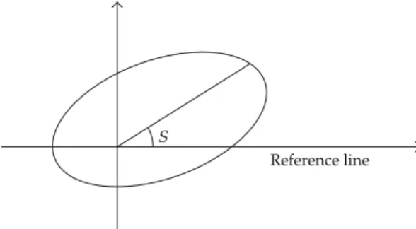
anomaly of the spacecraft;𝑠= range angle of the spacecraft;

(3)

Reference line S

Figure 1: Definition of the range angle and the arbitrary reference line.

The range angle “𝑠” is the independent variable of this

work and, it is the angle between the radius position vector of the satellite and a reference arbitrary line, which lies in the

plane of the orbit, as shown inFigure 1. It replaces the time in

the equations of motion.

There are also two important angles, pitch and yaw, which are used to define the direction of the thrust. The angle of

pitch is designated by𝐴, while the angle yaw is designated by

𝐵. The pitch is the angle between the thrust direction and the

perpendicular to the radius of the spacecraft, while yaw is the angle between the thrust direction and the orbital plane. The state variables used here are defined as follows [26–29]:

𝑋1= 𝑎 (1 − 𝑒 2₎

𝜇 ,

𝑋2= 𝑒cos(𝜔 − Φ) , 𝑋3= 𝑒sin(𝜔 − Φ) ,

𝑋4= fuel consumed_𝑚

0 ,

𝑋5=time,

𝑋6=cos( 𝑖2)cos(Ω + Φ_{2 ) ,}

𝑋7=sin( 𝑖2)cos(Ω − Φ_{2 ) ,}

𝑋8=sin( 𝑖2)sin(Ω − Φ_{2 ) ,}

𝑋9=cos( 𝑖2)sin(Ω + Φ_{2 ) ,}

(1)

where𝜇is the gravitational constant of the Earth and𝑚₀ is

the initial mass of spacecraft.

The advantage of using these state equations is to avoid singularities if the inclination or the eccentricity is zero. The equations of motion and the control variables used here are shown in [26–29]. The true longitude, which can be used as a constraint to define the prohibit region to apply the thrust, is given by

𝜆 = 𝜔 + 𝑣. (2)

The constraints on the final Keplerian orbital elements are given by (3). All the orbital elements are scaled. The desired

values are given by the index “∗”, while the suffix “₀” denotes

the initial value. The element without suffix or index is the current value of the element. The constraints on the final orbital elements are given by

(𝑎 − 𝑎∗₎ 󵄨󵄨󵄨󵄨𝑎0− 𝑎∗󵄨󵄨󵄨󵄨 = 0,

(𝑒 − 𝑒∗₎ 󵄨󵄨󵄨󵄨𝑒0− 𝑒∗󵄨󵄨󵄨󵄨 = 0,

(𝑖 − 𝑖∗₎ 󵄨󵄨󵄨󵄨𝑖0− 𝑖∗󵄨󵄨󵄨󵄨 = 0, (Ω − Ω∗₎ 󵄨󵄨󵄨󵄨Ω0− Ω∗󵄨󵄨󵄨󵄨 = 0,

(𝜔 − 𝜔∗₎ 󵄨󵄨󵄨󵄨𝜔0− 𝜔∗󵄨󵄨󵄨󵄨 = 0.

(3)

The Pontryagin’s maximum principle is used to find the optimal control that determinates the optimal trajectory. In this case, it is desirable to find the maximum final mass of

the spacecraft, given by the functional𝐽(⋅) = −𝑋₄(𝑠_𝑓). This is

equivalent of minimizing the fuel consumption, because the expenditure of fuel is the only way that the satellite has to lose mass. More details of this process can be found in [26–29]. The formulation of the problem is given by (4) to (6).

Maximize −𝑋₄(𝑠_𝑓) , (4)

with respect to 𝑠₀, 𝑠_𝑓, 𝐴₀, 𝐵₀, 𝐴󸀠₀, 𝐵󸀠₀, 𝑃_𝑖(𝑠₀) , (5)

subjected to 𝑆_𝑗(𝑋 (𝑠_𝑓)) = 0, 𝑗 = 1, . . . , 𝑚, (6)

where𝑆_𝑗(𝑋(𝑠_𝑓))are the constraints stated in (2) and (3) or

any other type.

Some of the initial variables that should be guessed are

the initial adjoint multipliers 𝑃_𝑖(𝑠₀). A good initial guess

for those variables is very important to assist convergence and to reduce the time the algorithm needs to obtain the solution. Unfortunately, the Lagrange multipliers do not have any physical meaning, so it is hard to find a good initial guess for them. To solve this problem, the adjoint-control trans-formation ([26–29]) is used to attribute a good estimative

for𝑃_𝑖(𝑠₀)from variables that have physical meaning. Those

variables are the angles𝐴₀and𝐵₀and the values of𝐴󸀠₀and

𝐵󸀠

0(Biggs [26], Prado [28]).

3. Steps of the Algorithm

The final complete algorithm has the following steps [28,29].

(i) It starts from an initial guess for the set of variables

(𝐴₀,𝐵₀,𝐴󸀠₀,𝐵󸀠₀,𝑠₀,𝑠_𝑓). With these initial values, the

(4)

(ii) The “adjoint-control” transformation is used to obtain the initial values of the Lagrange multipliers required for the numerical integrations.

(iii) Now, with all the initial values needed to solve the problem, the equations of motion and the adjoint equations are simultaneously numerically integrated during the propulsion arc. The values of the pitch and yaw angles are obtained, at every step of the inte-gration, by the principle of maximum of Pontryagin.

At the end, the value of the final state𝑋 after the

propulsion arc is obtained.

(iv) The Keplerian elements of the orbit achieved are then

obtained from the final state𝑋using (1).

(v) At this point, the satisfaction of the constraints is verified. If the magnitude of the vector that represents the constraints satisfaction is smaller than a specified tolerance provided by the user (the numerical zero), the algorithm proceeds to step (vii). On the other hand, if it is bigger, the algorithm proceeds to step (vi). (vi) At this step, the gradient of the constraints equations

(∇S) is obtained by perturbing the elements of the

control vectoruand performing a new set of

numer-ical integrations, in order to obtain the numernumer-ical derivatives of the constraints equations with respect

to the vectoru_{. Then, a new set of values for the vector}

u_{is found by (7) (Luemberger [33]) as follows:}

u_𝑖+1=u_𝑖− ∇S𝑇[∇S∇S𝑇]−1∇S (7)

and then the algorithm goes back to step (i), with the

new value of the vectoru_.

(vii) Once the constraints satisfaction is achieved, the next step is to search for the minimum of the fuel

consumed. The direction of the searchd,_{using the}

gradient method (Bazaraa et al. [34]), is

d= −R∇𝐽 (u) , ₍₈₎

where the vectorR_is

R=I− ∇S𝑇[∇S∇S]−1∇S. (9)

(viii) At this step, the magnitude of the vectord_{is verified.}

If it is smaller than a value specified by the user as a direction search tolerance (numerical zero), the algorithm goes to step (x) and if it is bigger, the algorithm proceeds to step (ix).

(ix) In order to get better results, the initial data “ratio of contraction” RC and the direction search tolerance

are reduced as u _{gets closer to the minimum. The}

magnitude for the direction search is then given by

PB= RC𝐽 (u)

∇𝐽 (u)d. (10)

So, the complete step is given by

u_𝑖+1 =u_𝑖+_PB d

|d|, (11)

and then the algorithm goes back to step (i).

(x) At this step, the possibility of the controlu _{to be a}

Kuhn-Tucker point is verified. To check this

condi-tion, the vector VT _{is built, formed by the} 𝑚 _first

elements of the vector given by (Bazarra et al. [34]) as follows:

W= −(SS𝑇)−1S∇𝐽 (u) , (12)

where𝑚is the number of active constraints. IfVT_is

not positive definite, the line𝑗, which causesVT_𝑗_to

be negative on the matrixS, is deleted. And then the

algorithm returns to step (v).

(xi) The current step is verified and, if it is not the last one, the algorithm goes to a new search for the minimum fuel consumption with a smaller direction search tolerance for the objective function. If this step is the last one, the algorithm is finalized.

4. Extensions of the Algorithm

There are several extensions of the algorithm that can be considered, in order to make it more flexible. The first one is the possibility to perform maneuvers with more than one arc of propulsion. Increasing the number of propulsion arcs means that the number of optimization variables is increased.

For example, for one thrust arc there are 𝑢₁ to 𝑢₆ control

variables. For two thrust arcs, similarly, there is a set of𝑢₁to

𝑢12control variables and so on. In addition, by adding more

than one thrust arc, the inclusion of constraints to prevent the overlap of thrust arcs becomes necessary.

Another extension is the possibility to consider forbidden regions to apply the propulsion as a constraint. These regions are defined by the true longitude, as shown in (2). Both values of the initial and final true longitudes of the prohibit region have to be specified.

In some situations, the initial range angles𝑠₀can be less

than zero. It means that when the thrust is started, the time is negative. To avoid negative time, it is added a constraint that

imposes to𝑠₀, the time, to be equal or bigger than zero. This

constraint is only active if𝑠₀< 0.

The last extension is the possibility to consider constraints restricting the pitch and yaw angles. In this case the bounds

considered on 𝐴and 𝐵 are the ones given by Biggs [27]:

𝐴𝐿 ≤ 𝐴 ≤ 𝐴𝑢 and 𝐵𝐿 ≤ 𝐵 ≤ 𝐵𝑢, where the suffix “𝑢”

represents the maximum angle and the suffix “𝐿” represents

the minimum angle. If these constraint are active after finding

the optimal angles𝐴∗and𝐵∗, and this problem is solved as

follows [26–29]:𝐴 = 𝐴_𝑢 if𝐴∗ ≥ 𝐴_𝑢,𝐴 = 𝐴_𝐿 if𝐴∗ ≤ 𝐴_𝐿,

𝐴 = 𝐴∗ _if _𝐴

𝐿 ≤ 𝐴 ≤ 𝐴𝑢. Those equations are similarly

applied to the optimal yaw angles𝐵∗.

5. The Permanent Magnet Hall Thruster

(5)

consumption. Although electric propulsion has low thrust, the high specific impulse guarantees a reduced burned fuel along the maneuver.

The hall thruster, used in this work as the propulsion system, was fundamentally envisaged in Russia in 1960, and the first successful space mission with this thrust propulsion with 60 mN was used in the Meteor satellite series in 1972 (Zhurin et al. [35]). After that, this kind of propulsion system has been studied and developed in several countries, such as France, USA, Japan, and Brazil.

The working principle of the hall thrusters is the use of an electromagnet to produce the main magnetic field responsible for the plasma acceleration and generation (Fer-reira et al. [30]). This configuration requires the use of energy to produce the magnetic field. Nevertheless, the permanent magnet hall thruster (PMHT) developed at the Plasma Laboratory of the Universidade de Brasilia uses an array of permanent magnets, instead of an electromagnet, to produce a radial magnetic field inside the cylindrical plasma drift channel of the thruster (Ferreira et al. [30]). The use of permanent magnets instead of electromagnet guarantees low-power consumption, and it can be used in small- and medium-size satellites (Ferreira et al. [30]).

In the Plasma Laboratory of the Universidade de Bras´ılia, it has been developed two kinds of hall thruster, called Phall I and Phall II. The first one to be constructed was the Phall I. It has a stainless steel chamber with 30 centimeters of diameter. Its magnetic field is produced by two concentric cylindrical arrays of ferrite permanent magnets: 32 bars in the outer shell and 10 bars in the inner shell. The magnetic field in the middle line of the plasma source’s channel is 200 Gauss (Ferreira et al. [30]). On the other hand, the second thruster Phall II has an aluminum plasma chamber and it is smaller, with 15 cm diameter, and contains neodymium-iron magnets to

produce the magnetic field (Ferreira et al. [30]).Table 1gives

the parameters of the performance of both Phall I and Phall II thrusters (Ferreira et al. [30]).

In this paper, it was found first the optimal maneuvers

with the thrust parameters shown in Table 1. Then, these

optimal maneuvers were simulated with a PID control for a long period of time, based on the continuous monitoring of the thrust in a real-time performance, correcting any possible failure.

6. Spacecraft Trajectory Simulator

The maneuver simulator used to simulate the optimal maneu-vers in a more realistic way is the spacecraft trajectory simulator (STRS). The STRS can consider constructional features and operation, such as nonlinearities, failures, errors, and external and internal disturbances, in order to determine the deviation in the reproduction of the optimal solution previously found.

Furthermore, maneuvers with continuous thrust are used during a long period of time. This kind of maneuvers requires a PID control system to guarantee the achievement of the final conditions of the maneuver. The operating structure of the STRS can be described as follows (Rocco [36]).

(a) The simulation occurs in a discrete way, that is, at every simulation step, the state of the vehicle (position and velocity) must be computed. For all purposes, the disturbances, nonlinearities, errors, and failures must be considered.

(b) Since a closed loop system was used to control the trajectory, the reference state is determined by applying the optimal maneuver. Then, the current state follows the reference but considers the effects of disturbances and the constructive characteristics of the vehicle.

(c) The difference between the reference state and the current state creates an error signal that is inserted into a PID control.

(d) The controller produces a control signal according to the PID control law and the gains that have been set. (e) The control signal is inserted into the actuator model

(propellant thrusters), where the nonlinearities inher-ent to the construction of the actuator can be consid-ered. Thus, the behavior of the propellant thrusters can be reproduced by the appropriate adjustment of the model parameters, which are supplied by the manufacturer of the thrust actuator.

(f) Finally, an actuation signal(Δ𝑉)is sent to the

dynam-ical model of the orbital motion. At this signal the velocities increments due to the disturbances can be added.

(g) With the actuation signal added with the possible dis-turbances, the model of the orbital dynamics provides the state (position and velocity) after the application of the propulsion.

(h) Through the use of sensors that were modeled con-sidering its constructive aspects, the current state is determined and compared with the reference state in order to close the control loop.

7. Results

Before performing tests with the propulsion system Phalls I and II, that is one of the goals of the present paper, it is important to test some of the particular characteristics of the algorithm developed here. Those tests are performed in maneuvers that have similar results available in the literature, so a comparison to validate the algorithm and the software developed can be made. After that, the results of the optimal maneuvers using the new propulsion devices, as well as the simulations of them in the STRS, are presented.

7.1. Optimal Maneuvers to Validate the Algorithm

7.1.1. Maneuver 1. This first maneuver described has a con-straint at the pitch angle, in order to test this capability of the proposed algorithm.

Initial orbital elements:

𝑎= 99000 km;𝑒= 0.7;𝑖= 10∘;Ω= 55∘;𝜔= 105∘;𝑣=

(6)

Table 1: Comparative performance parameters measured in PHALL I and PHALL II.

PHALL1 PHALL2

Maximum expected thrust (mN) 126 126

Average measured thrust (mN) 84,9 120,0

Thrust density (N/m2) 4,68 <6,0

Maximum specific impulse (s) 1607 1607

Measured specific impulse (s) 1083 1600

Ionized mass ratio (%) 3,3 ∼30

Propellant consumption (Kg/s) 6, 0 × 10−6 1, 0 × 10−6

Energy consumption (W) 350 250–350

Electrical efficiency (%) 33,9 60

Total efficiency (%) 10,12 50,0

Range angle (degrees)

Pitch (degrees)

110 100

90 80 0 1 2 3 4 5

120 130 140

−1

−2

−3

−4

−5

Figure 2: Optimal pitch angles of the maneuver 1.

Vehicle mass = 300 kg; thrust = 1.0 Newton, initial

position𝑠= 0∘.

Condition on the final orbit:𝑎= 104000 km.

Other constraints: 5∘≥ 𝐴 ≥ −5∘(pitch constraint).

Final orbital elements obtained after the maneuver:

𝑎= 103999.21 km;𝑒= 0.7143;𝑖= 10∘;Ω= 55∘;𝜔= 105∘;

𝑣= 30.24∘.

Fuel consumption: 2.4235 kg; fuel consumption in Biggs [27]: 2.44 kg; fuel consumption in Prado [28]: 2.45 kg.

Figure 2shows the direction of the thrust.

Now, with the constraint in the direction of propulsion, the fuel consumption was increased when compared with

a maneuver without this constraint [27,28]. The extra fuel

needed due to this constraint is 3.8×10−3kg. It is possible to

view clearly that the pitch angle is confined to 5∘at the end

of the maneuver. In any case, the algorithm developed here obtains better results when compared to Biggs [27] and Prado [28].

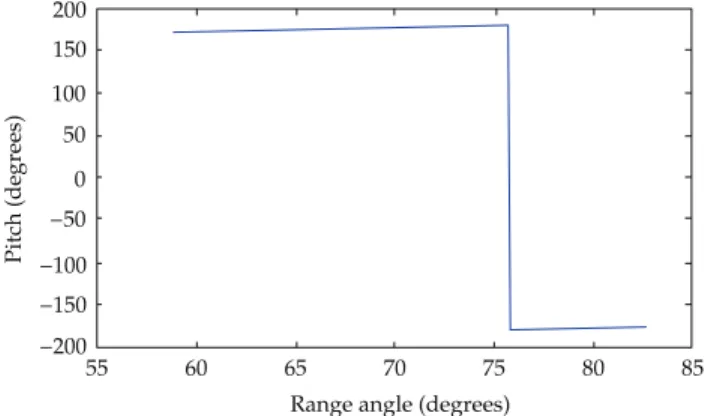
7.1.2. Maneuver 2. This maneuver has the constraint of a region prohibited for thrusting. This is one of the most important capabilities of the algorithm developed here.

𝑎= 99000 km;𝑒= 0.7;𝑖= 10∘;Ω= 55∘;𝜔= 105∘;𝑣=

−105∘.

Pitch (degrees)

55 50 45 40 35 30

25 60 65 70

−20

−21

−22

−23

−24

−25

−26

−27

−28

−29

−30

Figure 3: Optimal pitch angles of the maneuver 2.

position𝑠= 0∘.

Condition on the final orbit:𝑎= 104000 km.

Other constraints: no thrust between the true

longi-tudes 120∘and 180∘.

Final orbital elements:

𝑎= 103999.85 km;𝑒= 0.7134;𝑖= 10∘;Ω= 55∘;𝜔= 105∘;

𝑣= 320.80∘.

Figure 3shows the direction of the thrust.

InFigure 3it is possible to note that the solution has the

thrust arc ending in𝜆= 120∘. The true longitude is defined

here as𝜆 = 𝜔 + 𝑣 = 425.80∘, that is similar to 65.80∘, that is

the result shown inFigure 3. In this way, the region prohibit

of thrust was obeyed and, compared with the maneuver that is free of this constraint, the extra fuel needed to reach the final semimajor axis required was 0.3655 kg. Once again, the algorithm proposed here obtained better results when compared to Biggs [27] and Prado [28].

7.1.3. Maneuver 3. This maneuver has the requirements of changing three orbital elements of the orbit at the same time.

𝑎= 41904.1 km;𝑒= 0.018;𝑖= 0.688∘;Ω=−29.8∘;𝜔=

(7)

Pitch (degrees)

75 70 65 60

55 80 85

200

150

100

50

0

−50

−100

−150

−200

Figure 4: Optimal pitch angles of the maneuver 3 for the first arc.

Yaw (degrees)

Range angle (degrees) 75 70 65 60

55 80 85

−61.2

−61.4

−61.6

−61.8

−62

−62.2

−62.4

−62.6

Figure 5: Optimal yaw angles of the maneuver 3 for the first arc.

position𝑠= 0∘.

Condition on the final orbit:𝑎= 42164.2 km;𝑒= 0;

𝑖= 0∘.

Final orbital elements:

𝑎= 42164.55 km;𝑒= 0.00130;𝑖= 0.0419∘;Ω= 300.60∘;

𝜔= 100.47∘;𝑣= 143.64∘.

Figures4–7show the direction of the thrust.

In this maneuver there are three Keplerian elements fixed on the final orbit: semimajor axis, eccentricity, and inclination. Since the maneuver includes a change in the orbital plane, the yaw angle is not zero. The final conditions were satisfied and the fuel consumption was reduced by 0.014 kg, when compared to Prado [28].

7.2. Optimal Maneuvers Using the Phalls I and II. In this section we present the optimal maneuvers found by the algorithm presented in the present paper when using Phalls I and II. The optimal thrust angles are presented, and the specific impulse considered for each maneuver is given in

Table 1. Figures 8–23 present the optimal angles for the

proposed maneuvers given by the initial and final range angle and the pitch angle at each arc of propulsion. The yaw angle is always zero, because all the maneuvers simulated are planar.

Pitch (degrees)

215 205 210 200

190 195

185 220 225

30

25

20

15

10

5

0

−5

Figure 6: Optimal pitch angles of the maneuver 3 for the second arc.

Yaw (degrees)

215 205 210 200

190 195 185

60

55

50

45

40

35

30

220 225

Figure 7: Optimal yaw angles of the maneuver 3 for the second arc.

All the maneuvers considered here have the same initial orbital elements and final condition imposed for the final orbit. Only the number of arcs and the propulsion system is different at each maneuver. The parameters of the maneuver proposed are as follows.

Initial orbital elements:𝑎= 7130.865 km;𝑒= 0.0035;𝑖

= 98.5054∘;Ω= 0∘;𝜔= 0;𝑣= 220∘.

Vehicle mass = 300 kg.

Condition imposed on the final orbit:𝑎= 7200 km;𝑒

= 0.004.

7.2.1. Maneuver 4. For this maneuver it was considered the existence of three Phall I thrusters. The propulsion force of each one is assumed to be the average measured value. The parameters considered in this maneuver are as follows.

Total thrust = 0.252 Newton; specific impulse: 1083 s.

Solution:

Final orbital elements:𝑎= 7200.00 km;𝑒= 0.004.

Fuel consumption: 1.046346 kg. Duration of the maneuver: 44066.96 s.

(8)

3000 2500 2000 1500 1000 500

Pitch angle (degrees)

0 0 5 10 15

−10

−15

−5

Figure 8: Optimal pitch angles for maneuver 4.

0.3

0.1 0 0.2 0.4 0.5

1400 1200 1000 800 600 400 200 0

−0.1

−0.2

−0.3

−0.4

−0.5

Figure 9: Optimal pitch angles for the first arc of the maneuver 5.

1

0 0.5 1.5 2

4000 3800 3600 3400 3200 3000 2800 2600

−0.5

−1

−1.5

−2

Figure 10: Optimal pitch angles for the second arc of maneuver 5.

Solution:

Final orbital elements after the first arc: 𝑎 =

7165.30 km;𝑒= 0.0039.

Final orbital elements after the second arc: 𝑎 =

7200.00 km;𝑒= 0.0040.

Note that the use of two arcs generates savings in the fuel consumption, as expected.

0 5 10 15

2200 1800 2000 1600

1400 1000 1200 800

600 400 200

−5

−10

−15

Figure 11: Optimal pitch angle for maneuver 6.

0.2

0 0.6 0.4 0.8 1

1000 900 600 700 800 500

400 300 200 100 0

−0.2

−0.6

−1

−0.4

−0.8

Figure 12: Optimal pitch angles for the first arc of maneuver 7.

0 0.5 1 1.5

2400 2300 2100 2200 2000

1900 1800 1700 1600 1500

−0.5

−1

−1.5

Figure 13: Optimal pitch angles for the second arc of maneuver 7.

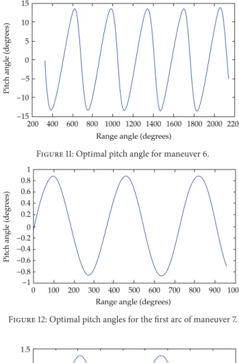
7.2.3. Maneuver 6. For this maneuver it was considered the existence of three Phall II thrusters. The propulsion force of each one is assumed to be the average measured value. The parameters considered in this maneuver are as follows.

Solution:

(9)

Time (s)

−5

−10

0

0 5

0.5 1 1.5 2 2.5 3 3.5 4 4.5

×104

Semimajor axis deviation

(

m

)

Figure 14: Semimajor axis deviation in maneuver 4.

0 2 4 6 8 10 12

Time (s)

0 0.5 1 1.5 2 2.5 3 3.5 4 4.5

×104

−2

−4

−6

−8

Eccentricity deviation

×10−7

Figure 15: Eccentricity deviation in maneuver 4.

0 0.005 0.01 0.015

Position deviation (m)

Time (s)

0 0.5 1 1.5 2 2.5 3 3.5 4 4.5

×104

−0.005

−0.01

Figure 16: Position deviation in maneuver 4.

Note that the use of the Phall II generates savings in the fuel consumption since it has better parameters when compared to the Phall I device.

7.2.4. Maneuver 7. This maneuver has the same conditions of maneuver 6, but now with two thrust arcs instead of one. The parameters considered in this maneuver are as follows.

Solution:

7167.77 km;𝑒= 0.0039.

0 1 2 3 4 5

Velocity deviation (m/s)

Time (s)

0 0.5 1 1.5 2 2.5 3 3.5 4 4.5

×104

−1

−2

−3

×10−3

Figure 17: Velocity deviation in maneuver 4.

7200.00 km;𝑒= 0.0040.

Note that the use of two arcs generates savings in the fuel consumption one more time, as expected.

7.3. Optimal Maneuvers Simulations Using the STRS. Now, with the help of the optimal maneuvers found previously, we shall simulate those maneuvers in the STRS using the optimal angles. Some different aspects of the propulsion system were considered to simulate a more realistic environment, and also the PID control was considered.

In this section, for the propulsion system, it was

consid-ered that at each inertial direction𝑥,𝑦,𝑧has an error on the

actuator signal (m/s) with mean equal to zero and variance

equal to 10−10, that is, it was inserted an error in the velocity of

the satellite. This error has amplitude approximately close to 5

×10−3N for each thrust, which corresponds to the error of the

PMHT (Ferreira et al. [30]). There is a PID control to correct the errors due the actuator, but it is still possible to analyze the deviations and the increase of the fuel consumption due to the errors.

7.3.1. Maneuver 4 in STRS. In this case it is considered maneuver 4, including the solution found there.

Fuel consumption: 1.0470 kg.

Propellant mass difference from the optimal

maneu-ver: 6.66×10−4kg.

The error inserted in the propulsion system resulted in a

deviation of the orbital elements, as we can see in Figures14

and15for the semimajor axis and eccentricity. If there was

not any error at the propulsion system, the deviation would

be zero all the time for the orbital elements. In Figures16and

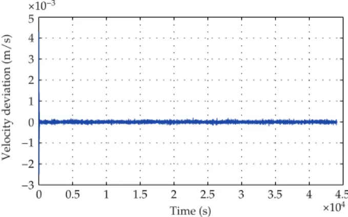
17we can see also the effect of the error in the velocity and

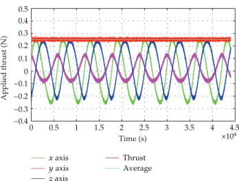
position, as a function of these parameters. Finally, the thrust

(10)

Applied thrust (N)

Time (s)

0 0.5 1 1.5 2 2.5 3 3.5 4 4.5

×104

0.5 0.4 0.3 0.2

0.1

0

−0.1

−0.2

−0.3

−0.4

xaxis

yaxis

zaxis

Thrust Average

Figure 18: Thrust applied in maneuver 4.

0 5 10

Time (s)

0 0.5 1 1.5 2 2.5 3 3.5

×104

−5

−10

−15

Semimajor axis deviation

(

m

)

Figure 19: Semimajor axis deviation in maneuver 6.

7.3.2. Maneuver 5 in STRS. In this case maneuver 5 is considered, including the solution found.

7165.23 km;𝑒= 0.0039.

7199.80 km;𝑒= 0.0040.

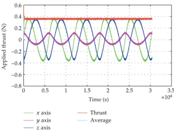
7.3.3. Maneuver 6 in STRS. Now maneuver 6 is considered.

The same analysis for the figures made inSection 7.3.1fits

here. Figures19–23show the deviations and the error that

occurred on the propulsion system.

Time (s)

0 0.5 1 1.5 2 2.5 3 3.5

×104

Eccentricity deviation

×10−6

2

1.5

1

0.5

0

−0.5

−1

−1.5

Figure 20: Eccentricity deviation in maneuver 6.

7.3.4. Maneuver 7 in STRS. Maneuver 7 is now studied.

7167.70 km;𝑒= 0.0039.

7199.83 km;𝑒= 0.0040.

7.3.5. Maneuver 8 in STRS. This maneuver uses the optimal angles given in maneuver 4 but includes the errors proposed for the propulsion system. In addition, it was considered other nonlinearities for the actuator: two seconds delay to respond the control signal; a rate limiter for the variation of the satelite velocity, which the absolute limit of the rate is 0.00025 m/s; dead zone where the propulsion system is not turned on if the required velocity increment is lower than 0.0002 m/s. Considering these nonlinearities for the propulsion system, the PID control was able to achieve the maneuver although the fuel consumption was slightly increased. The results for this simulation are as follows.

Propellant mass difference from the optimal maneu-ver: 0.081429 kg.

7.3.6. Maneuver 9 in STRS. The maneuver simulated here uses the optimal angles given in maneuver 6, with the errors proposed for the propulsion system. In addition, it was proposed the same nonlinearities (rate limiter, dead zone, and time delay) of maneuver 8. Considering these nonlinearities for the propulsion system, the PID control was able to achieve the maneuver although the fuel consumption was increased. The results for this maneuver are as follows.

(11)

Time (s)

0 0.5 1 1.5 2 2.5 3 3.5

×104

0.02

0.015

0.01

0.005

0

−0.005

−0.01

−0.015

Position deviation

(

m

)

Figure 21: Position deviation in maneuver 6.

Velocity deviation (m/s)

Time (s)

0 0.5 1 1.5 2 2.5 3 3.5

×104

8

6

4

2

0

−2

−4

×10−3

Figure 22: Velocity deviation in maneuver 6.

xaxis

yaxis

zaxis

Thrust Average

Time (s)

0 0.5 1 1.5 2 2.5 3 3.5

×104

0.6

0.4

0.2

0

−0.2

−0.4

−0.6

−0.8

Applied thrust (N)

Figure 23: Thrust applied in maneuver 6.

8. Conclusion

Primarily, this paper established an algorithm to solve the problem of orbital maneuvers using a low-thrust control for a spacecraft that is travelling around the Earth. Then, all the maneuvers studied in this paper were successfully solved with the final conditions and constraints proposed and with reasonable fuel consumptions.

It was possible to verify that maneuvers with more thrusting arcs consume less fuel, as expected. This occurs because the algorithm has more variables to optimize, so it is possible to reduce the fuel consumption.

The second part of this work was to simulate the optimal maneuvers found by the algorithm proposed here in a more realistic environment, which can consider errors on the actuator that was not considered in the search for the optimal maneuver.

The maneuvers simulated in the STRS were coherent with the optimal maneuvers, validating the integration of both softwares.

The error considered in the propulsion system opens the possibility to study how the system would react to those nonlinearities. Although errors were inserted in the propulsion system, the PID control was able to correct and accomplish the maneuver.

It is possible to analyze the shifts caused by the error as well as the deviations in semimajor axis and eccentricity. It is also possible to see that the propulsion thrust was not linear.

For the maneuvers shown in Sections7.3.5and7.3.6, some

nonlinearities of the propulsion system, such as a response time, a rate limiter and a dead zone for the actuator signal were considered. All these errors occur in real systems. With the help of the STRS it was possible to simulate these errors and analyze the maneuvers studied with more accuracy. The STRS has shown to be an efficient simulator, capable of simulating and studying optimal maneuvers in a more realistic environment and to analyze many nonlinearities not considered in the calculation of the optimal maneuver.

Evidently, the phall II was more efficient than the phall I, as noticed by comparing maneuver 4 with maneuver 6 and maneuver 5 with maneuver 7. This was expected, since the phall II has a higher specific impulse and a higher average propulsion thrust as well. Nevertheless, the PID control was able to control all the maneuvers and reaches the final orbital constraints.

References

[1] D. F. Lawden, “Minimal rocket trajectories,”ARS Journal, vol. 23, no. 6, pp. 360–382, 1953.

(12)

[3] V. V. Beletsky and V. A. Egorov, “Interplanetary flights with constant output engines,”Cosmic Research, vol. 2, no. 3, pp. 303– 330, 1964.

[4] A. A. Sukhanov, “Optimization of flights with low thrust,”

Cosmic Research, vol. 37, no. 2, pp. 182–191, 1999.

[5] A. A. Sukhanov, “Optimization of low-thrust interplanetary transfers,”Cosmic Research, vol. 38, no. 6, pp. 584–587, 2000. [6] A. A. Sukhanov and A. F. B. A. Prado, “A modification of the

method of transporting trajectory,”Cosmic Research, vol. 42, no. 1, pp. 107–112, 2004.

[7] A. A. Sukhanov and A. F. B. A. Prado, “Optimization of low thrust transfers in the three body problem,”Cosmic Research, vol. 46, no. 5, pp. 440–451, 2008.

[8] A. A. Sukhanov and A. F. B. A. Prado, “Optimization of transfers under constraints on the thrust direction: I,”Cosmic Research, vol. 45, no. 5, pp. 417–423, 2007.

[9] A. A. Sukhanov and A. F. B. A. Prado, “Optimization of transfers under constraints on the thrust direction: II,”Cosmic Research, vol. 46, no. 1, pp. 49–59, 2008.

[10] S. S. Fernandes and F. D. C. Carvalho, “A first-order analytical theory for optimal low-thrust limited-power transfers between arbitrary elliptical coplanar orbits,”Mathematical Problems in Engineering, vol. 2008, Article ID 525930, 30 pages, 2008. [11] R. A. Boucher, “Electrical propulsion for control of stationary

satellites,”Journal of Spacecraft and Rockets, vol. 1, no. 2, pp. 164– 169, 1964.

[12] D. N. Bowditch, “Application of magnetic-expansion plasma thrusters to satellite station keeping and attitude control mis-sions,” in Proceedings of the 4th Electric Propulsion Confer-ence AIAA-1964-677, pp. 64–677, The American Institute of Aeronautics and Astronautics, Philadelphia, Pa, USA, Augest-September 1964.

[13] S. R. Oleson, R. M. Myers, C. A. Kluever, J. P. Riehl, and F. M. Curran, “Advanced propulsion for geostationary orbit insertion and north-south station keeping,” Journal of Spacecraft and Rockets, vol. 34, no. 1, pp. 22–28, 1997.

[14] T. A. Ely and K. C. Howell, “East-west stationkeeping of satellite orbits with resonant tesseral harmonics,”Acta Astronautica, vol. 46, no. 1, pp. 1–15, 2000.

[15] C. Circi, “Simple strategy for geostationary stationkeeping maneuvers using solar sail,”Journal of Guidance, Control, and Dynamics, vol. 28, no. 2, pp. 249–253, 2005.

[16] P. Romero, J. M. Gambi, and E. Pati˜no, “Stationkeeping manoeuvres for geostationary satellites using feedback control techniques,”Aerospace Science and Technology, vol. 11, no. 2-3, pp. 229–237, 2007.

[17] V. Gomes and A. F. B. A. Prado, “Low-thrust out-of-plane orbital station-keeping maneuvers for satellites,”Mathematical Problems in Engineering, vol. 2012, Article ID 532708, 14 pages, 2012.

[18] B. L. Pierson and C. A. Kluever, “Three-stage approach to opti-mal low-thrust earth-moon trajectories,”Journal of Guidance, Control, and Dynamics, vol. 17, no. 6, pp. 1275–1282, 1994. [19] Y. J. Song, S. Y. Park, K. H. Choi, and E. S. Sim, “A lunar cargo

mission design strategy using variable low thrust,”Advances in Space Research, vol. 43, no. 9, pp. 1391–1406, 2009.

[20] S. A. Fazelzadeh and G. A. Varzandian, “Minimum-time earth-moon and earth-moon-earth orbital maneuvers using time-domain finite element method,”Acta Astronautica, vol. 66, no. 3-4, pp. 528–538, 2010.

[21] G. Mingotti, F. Topputo, and F. Bernelli-Zazzera, “Efficient invariant-manifold, low-thrust planar trajectories to the moon,”

Communications in Nonlinear Science and Numerical Simula-tion, vol. 17, no. 2, p. 817, 2012.

[22] J. R. Brophy and M. Noca, “Electric propulsion for solar system exploration,”Journal of Propulsion and Power, vol. 14, no. 5, pp. 700–707, 1998.

[23] D. P. S. Santos, A. F. B. A. Prado, L. Casalino, and G. Colasurdo, “Optimal trajectories towards near-earth-objects using solar electric propulsion (sep) and gravity assisted maneuver,”Journal of Aerospace Engineering, Sciences and Applications, vol. 1, no. 2, pp. 51–64, 2008.

[24] D. P. S. Santos, L. Casalino, G. Colasurdo, and A. F. B. A Prado, “Optimal trajectories towards near-earth-objects using solar electric propulsion (sep) and gravity assisted maneuver,”

WSEAS Transactions on Applied and Theoretical Mechanics, vol. 4, no. 3, pp. 125–135, 2009.

[25] D. P. S. Santos and A. F. B. A. Prado, “Optimal low-thrust trajectories to reach the asteroid apophis,”WSEAS Mechanical Engineering Series, vol. 7, pp. 241–251, 2012.

[26] M. C. B. Biggs,The Optimization of Spacecraft Orbital Manoeu-vres. Part I: Linearly Varying Thrust Angles, The Hatfield Polytechnic, Numerical Optimization Centre, 1978.

[27] M. C. B. Biggs,The Optimisation of Spacecraft Orbital Manoeu-vres. Part II: Using Pontryagin’s Maximum Principle, The Hat-field Polytechnic. Numerical Optimization Centre, 1979. [28] A. F. B. A. Prado,Análise, Seleção e Implementação de

Procedi-mentos que visem Manobras Ótimas de Satélites Artificiais [M.S. thesis], Instituto Nacional de Pesquisas Espaciais, São José dos Campos, 1988.

[29] T. C. Oliveira,Estratégias ótimas para manobras orbitais uti-lizando propulsão cont´ınua [M.S. thesis], Instituto Nacional de Pesquisas Espaciais, São José dos Campos, 2012.

[30] J. L. Ferreira, G. C. Possa, B. S. Moraes et al., “Permanent magnet hall thruster for satellite orbit maneuvering with low power,”

Advances in Space Research, vol. 01, pp. 166–182, 2009. [31] E. Stuhlinger,Ion Propulsion for Space Flight, McGraw-Hill, New

York, NY, USA, 1st edition, 1964.

[32] R. G. Jahn,Physics of Electric Propulsion, McGraw-Hill, New York, NY, USA, 1st edition, 1968.

[33] D. G. Luemberger, Linear and Non-Linear Programming, Springer Science & Business Media, New York, NY, USA, 3rd edition, 2008.

[34] M. S. Bazaraa and C. M. Shetty,Nonlinear Programming-Theory and Algorithms, John Willey & Sons, New York, NY, USA, 1979. [35] V. V. Zhurin, H. R. Kaufman, and R. S. Robinson, “Physics of closed drift thrusters,”Plasma Sources Science and Technology, vol. 8, no. 1, pp. R1–R20, 1999.

(13)