Key words: Dividend; Arbitrage; Market equilibrium; Transactions costs; Taxes JEL classification: G12; G14

Carlos Pestana Barros & Nicolas Peypoch

A Comparative Analysis of Productivity Change in Italian and Portuguese Airports

WP 006/2007/DE _________________________________________________________

Maria Rosa Borges

An Arbitrage Model for the

Stock Price Adjustment in the Dividend Period

WP 009/2007/DE/CIEF _________________________________________________________

Departament of Economics

W

ORKING

P

APERS

ISSN Nº0874-4548

An Arbitrage Model for the

Stock Price Adjustment in the Dividend Period

Maria Rosa Borges

School of Economics and Management (ISEG) Technical University of Lisbon (UTL)

mrborges@iseg.utl.pt

Abstract

Following a dividend distribution, investors expect the stock price to decrease on the ex-dividend day. With no market imperfections, the price decrease should exactly match the amount of the dividend, thus eliminating all opportunities for profitable arbitrage. Allowing for different taxes on dividends and on capital gains results in a stock price adjustment ratio different from one, but there is still a unique equilibrium. With a simple model, considering four types of investors, we show that the consideration of transaction costs results in multiple possible equilibria (equilibrium zone), defined by the arbitrage boundaries of each type of investors. We also show that trading activity by the different types of investors is reflected in abnormal trading volume.

Key words: Dividend; Arbitrage; Market equilibrium; Transactions costs; Taxes

Introduction

The model developed in this paper analyzes the equilibrium conditions for the stock

price adjustment after a dividend distribution, in the context of imperfect markets, considering

the existence of taxes and transaction costs, and assuming that arbitrage activity leads prices

to equilibrium. This arbitrage model is inspired by the pioneering work of Elton and Gruber

(1970) as well as other authors including Kalay (1982), Eades Hess and Kim (1984),

Lakonishok and Vermaelen (1986) and Michaely (1991).

An investor that sells his stock before the payment of the dividend looses the right to

receive that dividend. If he sells his stock after the payment of the dividend, he receives the

dividend but, under arbitrage, he expects the stock price to decrease to a level that would

make him indifferent to sell before or after the dividend distribution. With no market

imperfections, the price decrease would exactly match the amount of the dividend. If we

allow for taxes and transaction costs in a market with rational arbitrage, the price decrease

after the dividend event should reflect the relative taxation of dividends and capital gains, as

well as the costs inherent to stock transactions.

Several papers study the effect of dynamic trading strategies around the ex-dividend

day. These strategies imply that investors trade around the ex-dividend day in order to avoid

or to capture the dividend, depending on their preferences for dividends or capital gains.

Kalay (1982) argued that, without risk or transaction costs, investors with the same taxes on

dividends and capital gains would buy the stock cum-dividend and sell ex-dividend, forcing

the stock price down by the amount of the dividend. This is consistent with the findings of

recognizes that transaction costs should be taken into consideration with the implication that

the price adjustment ratio would no longer be constrained to being equal to one. The author

argues that only within the boundaries defined by transaction costs would it be possible to

infer the marginal investor’s income tax as beyond those limits the price change would be

affected by arbitrage from investors seeking to take advantage of the opportunity to obtain

excessive returns. Only within the boundaries defined by (3), there are no arbitrage

opportunities. Miller and Scholes (1982) presented a similar argument in which the detected

relationship between dividend yield and price change subsequent to a dividend distribution

can be explained by short term trading as an alternative to the clientele effect explanation.

Eades et al. (1984) studied the behavior of prices around the ex-dividend day and

showed the existence of abnormal returns on days other than the ex-day. This is contrary to

the tax-induced clientele hypothesis as the tax effect explains only the price change on the

ex-day and not the behavior of prices around the ex-ex-day. The results of Kalay (1982) are

consistent with the findings of Karpoff and Walking (1988) who detect a significant

relationship between ex-day returns and transaction costs. Boyd and Jagannathan (1994)

develop a model with different types of investors facing different transaction costs before

showing how the relationship between the ex-day price change and dividend-yield is

non-linear. Lakonishok and Vermaelen (1986) confirm the presence of short-term traders in the

market around the ex-dividend day, detectable because of high or abnormal volumes. These

are more pronounced in high-yield stocks and Michaely and Vila (1995) set out an inverse

relation between transaction costs and abnormal volume. The evidence of high or abnormal

volumes around the ex-day is contrary to the static clientele models. Naranjo et al. (1998)

re-examined and extended the work of Eades et al. (1984) and find that the high-yield stock

ex-day returns are highly influenced by corporate dividend capture. Other insightful studies

The main contribution of our model is to extend theoretically on this discussion, by

defining the equilibrium conditions for different types of investors, considering taxes,

transaction costs and rational arbitrage. The general equilibrium will be defined by a range of

potential equilibrium points (the equilibrium zone), that will depend on the relative weights of

the different types of investors. We show that there is a relation between investor typologies

and the pattern of trading volume in the dividend period, which may help identifying the types

of investor that are present in the market.

Hypothesis

The hypotheses of the model are the following: (i) We assume that prices are

stationary around the dividend event. This implies that daily returns are expected to be zero

and that new information does not arrive to the market in that period. (ii) Investors maximize

expected return, when deciding to buy or sell stocks. Any expected profit opportunity will be

explored by investors. (iii) Investors are rational and form unbiased expectations about future

prices. Investors do not commit systematic errors in their predictions about future price

behavior. (iv) Investors are risk neutral. Decisions to buy and sell are only determined by

expected returns. Between two alternatives, investors will always choose that which has

higher expected return, independently of risk. Investors are indifferent between two

alternative strategies if they have the same expected return, whatever the risk of each

alternative. (v) Information is public and free. In the dividend period, all investors are fully

informed about the dividend amount, the distribution date, transaction costs, and taxation on

Under these hypotheses, and considering the absence of taxes and transaction costs,

there is market equilibrium when the expected price adjustment on the ex-day equals the

dividend amount, resulting in an expected return of zero.

(

)

1

= − D

P P_{b a}e

(1)

0

= + − =

b b e a e

P D P P

R (2)

where Re is the expected return, Pb is the stock price before the dividend, Pea is the expected

stock price after the dividend and D is the dividend. Allowing for market imperfections,

namely taxes and transaction costs, we add three other assumptions to our model: (vi)

Dividends are taxed, and the tax rate is assumed to be equal for all investors. (vii) Capital

gains are also taxed, and the tax rate is assumed to be equal for all investors. (viii) Every buy

or sell transaction has a positive transaction cost tax, independent of the trading volume, and

equal for all investors. With these additional assumptions, the equilibrium conditions (1) and

(2) are no longer valid, as will be shown in the next sections.

Effects from the Behavior of Different Types of Investors

The price adjustment after the dividend event will depend on the types of investors

that are present in the market during the dividend period. We consider four types of investors.

The first two have already made the decision to buy or to sell the stock, independently of the

dividend event. Investors type S want to sell, while investors type B have decided to buy

stocks. These investors now have only to decide the timing of the transaction, before or after

the dividend. The other two types of investors are arbitrageurs that will decide to make a

round-trip transaction, if they expect to obtain a positive return. Investors type BS buy stocks

and consider selling before the distribution date and buy them again after the event. We

assume that the actions of these four types of investors will force the stock price to adjust to a

level where profit opportunities become inexistent, for all of them. We will now determine the

equilibrium conditions for each type of investor.

Investors Type S

Investors type S will sell before the dividend distribution if the expected result is

positive:

(

)

(

)

(

)

[

−P_c 1+t_tc +P_b 1−t_tc −t_cg P_b −P_c

]

−

(

)

(

)

(

)

(

)

[

−P_c 1+t_tc +P_ae1−t_tc −t_cg P_ae −P_c +D1−t_d

]

>0 (3)

where the new variables have the following meaning: Pcis the stock acquisition price, td is the

dividend tax, tcg is the capital gains tax and ttcis the transaction cost tax. The first part of (3) is

the net result of selling before the dividend, and the second part is the net result of selling

after the dividend. From (3) we obtain:

(

)

tc cg

d e

a b

t t

t D

P P

− −

− > −

1 1

(4)

If condition (4) holds, investors type S will prefer to sell before the dividend, forcing

the price Pb to decrease. But if the inequality (4) is the opposite, investors type S will prefer to

sell after the dividend, forcing Pea down. Arbitrage by this type of investors will force prices

to adjust until the following equilibrium is reached:

(

)

tc cg

d e

a b

t t

t D

P P

− −

− = −

1 1

Investors Type B

Investors type B will buy stocks before the dividend, if they expect (6) to be positive:

(

)

(

)

(

)

(

)

[

− − + − − + e − _tc

]

−

s b e s cg tc b

d P t t P P P t

t

D1 1 1 (6)

(

)

(

)

(

)

[

−P_ae 1+t_tc −t_cg P_se−P_ae +P_se 1−t_tc

]

>0

where, Pes is the price that these investors will sell the stock in the future1. From (6) we obtain

the following condition:

(

)

tc cg d e a b t t t D P P + − − < − 1 1 (7)

Investors type B will buy stocks before the dividend if condition (7) holds, forcing Pb

to increase. If inequality (7) does not hold, investors type B will buy stocks after the dividend

and, in this case, Pea will increase. Again, the actions of these investors will lead to an

equilibrium condition:

(

)

tc cg d e a b t t t D P P + − − = − 1 1 (8)

Investors Type BS

Investors type BS are short term traders following a strategy of buying before the

dividend and selling after, if they believe they can make a profit:

0 ) ( ) 1 ( ) 1 ( ) 1

( + + − + − − − >

− e _b

a cg tc e a d tc

b t D t P t t P P

P (9)

From (9), we obtain a necessary condition for these short term traders to enter the market:

D P P t t t t D P

P _{b a}e

cg tc cg d e a b + − − − − < − 1 1 1 (10) 1

Or we could think of Pes as representing all future inflows from the stock, including dividends and capital

gains. We do not need to worry about the precise calculation of Pev because this variable cancels out in (7), and it

If there is this an arbitrage opportunity, these investors will buy before the dividend,

forcing an increase in Pb, and sell after the dividend, pushing down Pea. The combination of

this opposite movements in prices will remove profit opportunities, until:

D P P t t t t D P

P _{b a}e

cg tc cg d e a b + − − − − ≥ − 1 1 1 (11)

Investors Type SB

Finally, investors type SB will sell before the dividend and buy after, if the expected

result of this behavior is higher than to the alternative of holding the stock in their portfolio:

(

)

[

− − −

]

+

[

− + −

(

−

)

]

+ e

(

− _tc

)

−

s e a e s cg tc e a c b cg tc

a t t P P P t t P P P t

P (1 ) (1 ) 1

(

)

(

)

(

)

[

− − + 1− + e 1− _tc

]

>0

s d c

e s

cg P P D t P t

t (12)

Investors type SB obtain a profit if (13) holds:

D P P t t t t D P P e a b cg tc cg d e a b + − + − − > − 1 1 1 (13)

If this arbitrage opportunity exists, the actions of investors type SB force Pb to decrease and

Pea to increase, reducing profits which will disappear when:

D P P t t t t D P

P _{b a}e

cg tc cg d e a b + − + − − ≤ − 1 1 1 (14)

Arbitrage and Equilibrium

opportunities for each type of investor, given by (5), (8), (11) e (14), simplifies to the

equilibrium condition of Elton and Gruber (1970):

(

)

cg d e

a b

t t D

P P

− − = −

1 1

(15)

Positive transaction costs have, however, a significant impact on the equilibrium conditions,

with different boundaries for the arbitrage opportunities. Figure 1 identifies profit

opportunities for the different types of investors and the arrows show the impact of their

actions on the expected price adjustment.

Figure 1

Boundaries of Arbitrage Zones

All boundaries are defined in relation to the central value given by (15). Between

boundaries B and S, investors types S and B, force the price adjustment in opposite directions.

The location of the equilibrium depends on the relative forces of the two types of investors,

but it certainly will fall in the interval define by these two boundaries:

    

  

− −

− +

− −

tc cg

d

tc cg

d

t t

t t

t t

1 1 ; 1

1

For investors types SB and BS, there are no profit opportunities inside boundaries SB and BS,

that is, in:

        ₊ − + − − + − − − − D P P t t t t D P P t t t

t _{b a}e

cg tc cg d e a b cg tc cg d 1 1 1 ; 1 1 1 (17)

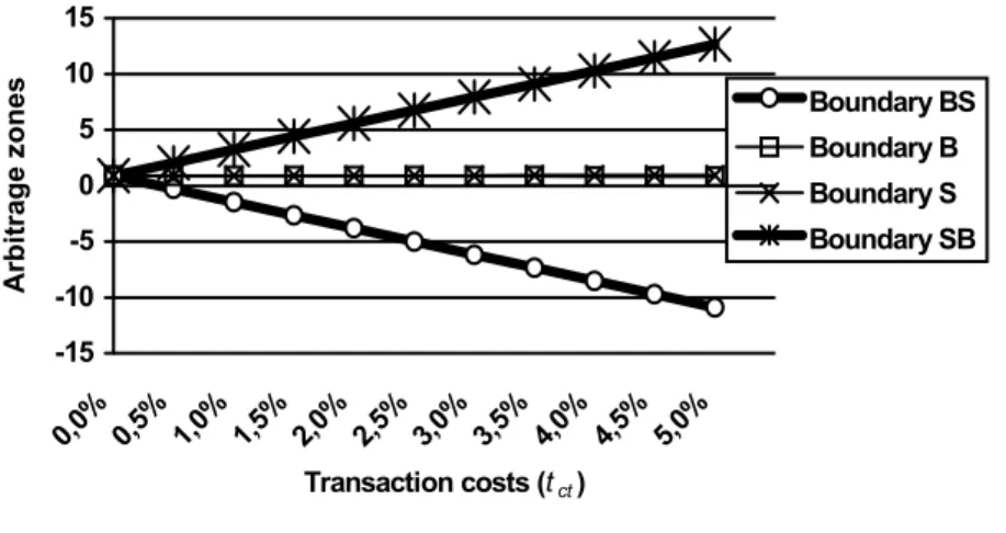
Figure 1 assumes that (16) is narrower than (17). There is no general proof of this

result. However, if we restrict ourselves to combinations of td, tcg, ttc and D/P which are close

to values observed in the real world, interval (16) will be much smaller than interval (17). In

Figure 2, using td=25%, tcg=15%, D/P=1%, interval (17) is more than 200 times wider than

interval (16), for any transaction cost, ttc, between 0% and 5%.

Figure 2

Sensitivity of Arbitrage Boundaries to Transaction Costs

-15 -10 -5 0 5 10 15

0,0% 0,5% 1,0% 1,5% 2,0% 2,5% 3,0% 3,5% 4,0% 4,5% 5,0%

Transaction costs (t_ct)

Arb itrag e z o ne s Boundary BS Boundary B Boundary S Boundary SB

This result is not surprising, because transaction costs have a very different impact on

investors type B and S, on one side, and investors BS and SB, on the other. While investors B

and S only face costs from one transaction, investors SB and BS will pay the costs of two

irrelevant for their decision. The difference in transaction costs, between their two

alternatives, to transact before or after the dividend, is given byt_tc

(

P_b −P_ae

)

.

Equilibrium

If profit opportunities are totally explored the price adjustment will be inside

boundaries S and B, where all points are a possible equilibrium solution. Here, the actions of

investors S and B push the price in opposite directions, and the final equilibrium will depend

on the relative strengths of these two types of investors. Note that none of the investors is

individually in equilibrium, because profit opportunities have not been completely exhausted.

In any case, both types of investors choose to delay buying/selling until after the dividend

distribution. This means that, ceteris paribus, we should observe a positive abnormal

transaction volume after the distribution event and a negative abnormal volume before. If the

price adjustment falls outside boundaries S and B, this means that the actions of investors S

and B are not sufficient to explore all profit opportunities, by reasons unrelated to taxes and

transaction costs. This may happen if these types of investors exist in small numbers in the

market, and so they would not have a strong enough influence over prices.

Investors types BS and SB do not intervene if the price adjustment is within boundaries

BS and SB. The profit opportunities for these investors exist only below boundary BS and

above boundary SB, respectively. The activity of these investors will lead to abnormal

transaction volume both before and after the dividend. An important aspect is the extreme

sensitivity of arbitrage opportunities for investors SB and BS, to the dividend yield, when

transaction costs are positive. If we take td=tcg, D/P=1% e ttc=0.5%, the transaction costs of a

exist for investors BS if P_b−P_ae <0, and for investors SB if

(

P_b−P_ae

)

/D>2. Figure 3 shows

how boundaries SB and BS get wider as dividend yield lowers and transaction costs increase.

Figure 3

Sensitivity of Arbitrage Boundaries SB and BS to ttcand D/P

-10 -9 -8 -7 -6 -5 -4 -3 -2 -1 0 1 2 3 4 5 6 7 8 9 10 Dividend yield P ri ce a d ju st m en t 2% 0%

SB tct=1,5%

SB tct=0,5%

BS tct=0,5%

BS tct=1,5% BS tct=0,1%

SB tct=0,1%

Expected Pre-tax Returns in Equilibrium

In equilibrium, after-tax returns are zero. With taxes and transaction costs, investors

will demand positive pre-tax returns. We obtain these equilibrium pre-tax returns by equaling

(5), (8), (11) and (14) to zero, for all types of investors:

Type S:

(

₍

₎

)

b tc cg tc cg d b b e a e S P D t t t t t P D P P R − − − − = + − =

1 (18)

Type B:

(

₍

₎

)

b tc cg tc cg d b b e a e P D t t t t t P D P P RB + − + − = + − =

1 (19)

Type BS:

(

₍

₎

)

(

b

)

e a tc cg d b e a

e P P D t t D t P P

Type SB:

(

₍

₎

)

(

)

cg b e a tc b cg cg d b b e a e t P P t P D t t t P D P P RSB − + − − − = + − = 1 1

1 (21)

These conditions are the minimum pre-tax returns demanded by investors, and occur

when all arbitrage opportunities are exhausted. For investors types SB and BS, these

conditions represent the minimum return demanded to enter the market. If the following

condition does not hold:

(

)

(

)

(

cg

)

b e a tc b cg cg d b b e a e t P P t P D t t t P D P P RBS − + + − − > + − = 1 1

1 (22)

investor type BS will prefer not to enter the market. On the other hand, investor type SB will

stay out of the market unless:

(

)

(

)

(

cg

)

b e a tc b cg cg d b b e a e t P P t P D t t t P D P P RSB − + − − − < + − = 1 1

1 (23)

Generally, expected pre-tax equilibrium returns will be positive if td>tcg, and negative

if td<tcg, although we have to also consider transaction costs. Table I shows the impact on

pre-tax equilibrium returns for all types of investors, from changes in td, tcg, ttc and D/P. For all

investors, expected pre-tax returns increase with the tax rate on dividends. Conversely,

expected pre-tax returns will be lower as the tax on capital gains increases, for all investors

except for type BS, where the sign is ambiguous. The impact of transaction costs is negative

on the expected pre-tax return of investors S and SB, and positive on the expected pre-tax

return of investors B and BS. Finally, the relationship between expected pre-tax returns and

dividend yields will be positive for investors SB and BS, if

t

d

>

t

cg, for investors S, if

tc cg

d

t

t

t

>

+

, and for investors B, if

t

d

>

t

cg

−

t

tc. Normally,

t

tc is much smaller than

t

d

and

t

cg, so we will have a positive relationship between the expected pre-tax return and the

Table I

Impact of Changes in td, tcg, ttc and D/P on Pre-tax Equilibrium Returns

Effects of Differential Taxation

The previous analysis is based on the assumption that taxes are equal for all investors.

If we assume that investors may face different tax rates, there are some interesting points to

show. Consider

t

d

>

t

cg for all investors, except for investors type BS, who face equal tax

rates,

t

_d

=

t

_cg. With no transaction costs, arbitrage opportunities disappear for investors type

BS, if the price adjustment equals the amount of the dividend,

(

)

₁

1

1 ₌

− − = −

cg d e

a b

t t D

P P

.

For all other investors, we will have:

(

)

1 1

1 _{= <}

− − = −

e t

t D

P P

cg d e

a

b _.

Figure 4 shows the arbitrage boundaries under these assumptions. For transactions

final equilibrium will depend on the relative weight of all types of investors, but it will be

located in the shadowed area at the left of A.

Figure 4

Arbitrage Boundaries with Different Taxation

If transaction costs are between A and B, there will be divergent interests between investors

BS, on one side, and investors S and B, on the other. Once again, equilibrium will depend on

the relative weight of these investors and it will be located in the shadowed area between A

and B. If transaction costs exceed B, we will have the same case as in the model with identical

taxation for all investors, with the equilibrium located between boundaries B and S. This

example illustrates conflicts of interest between different types of investors, resulting from

different taxations. In the real world more complex equilibria certainly exist. This example is

useful because it shows that it is possible to have a global equilibrium where none of the

investors has explored all profit opportunities and so, is not individually in equilibrium.

Another implication is that the income tax rate of the marginal investor can not be inferred

Trading Volume in the Dividend Period

The trading volume will be affected by the actions of the different types of investors.

Depending on the equilibrium zone, we will observe different behaviors by investors, which

will affect transaction volume in different ways, as is graphically shown in Figure 5.

Let us consider the existence of profit opportunities for investors types BS and SB, that

is, the price adjustment is expected to fall in Zones Ia or Ib. In this case, we observe a positive

abnormal trading volume both before and after the dividend event, by these types of investors.

Investors BS will be active in zone Ia, while investors SB will be active in zone Ib. If the price

adjustment is expected to fall in zones Ia or IIa, investors B will anticipate transactions to

before the dividend and this translates in abnormal positive volume before the dividend and

negative after. Investors S will postpone their sales until after the dividend, thus having an

opposite effect on abnormal trading volume. The combined effect on trading volume depends

on the relative weights of the transactions made by these two types of investors. This rationale

can be extended to equilibrium zones IIb and Ib, where investors B and S change positions, in

terms of their impact on the abnormal trading volume, as investors B will sell after the

dividend and investors S will buy before the dividend.

Again the combined effect on abnormal trading volume is ambiguous as it depends on

the relative weights of both types of investors. If the price adjustment is expected to fall in

zone III, both investors types B and S postpone their transactions until after the dividend, thus

causing a negative abnormal volume before the dividend and a positive abnormal volume

after. Thus, the observation of the trading volume during the dividend period may be an

important indicator for the types of investors active in the market, affecting the level of price

Figure 5

Conclusions

With a simple model assuming very restrictive hypothesis, we show that the allowance

for market imperfections such as taxes and transactions costs implies that there is not a unique

equilibrium point for the level of stock price adjustment following a dividend distribution

event, but rather there are many possible equilibria. The main reason for this is the fact that

transaction costs limit the arbitrage opportunities and so there are boundaries below which (or

above which) arbitrage becomes unprofitable and so there are no market forces pushing the

price to a unique market equilibrium.

In the real world, where the spectrum of investors is more diverse than the four types

allowed for in the model, where: tax rates are different between investors; transaction costs

may be different for different agents; preferences regarding the trade-off between risk and

return are also heterogeneous; and arbitrage may be limited by infrequent trading, we should

expect to observe much more complex equilibria, and a wider range of possible values for the

stock price adjustment.

Finally, and in the absence of direct data regarding the identification of the types of

investors affecting the global equilibrium, we show that the observation of abnormal trading

volume around the dividend event may give us some insights on the identification of which

investors are present in the market.

References

Bartholdy, J.; Brown, K. “Testing for multiple types of marginal investor in ex-day pricing”, Multinational Finance Journal, 8, 2004, pp. 173-209.

Borges, M. “Short-term trading around dividend distributions: An empirical application to the Lisbon stock market”, Proceedings of European Applied Business Research Conference – EABR, Edinburgh Scotland, June 2004.

Eades, K.; Hess, P.; Kim, E. “On interpreting security returns during the ex-dividend period”, Journal of Financial Economics, 13, 1984, pp. 3-34.

Elton, E.; Gruber, M. “Marginal stockholder tax rates and the clientele effect”, Review of Economics and Statistics, 52, 1970, pp. 68-74.

Kadapakkam, P. “Reduction of constraints on arbitrage trading and market efficiency: An examination of ex-day returns in Hong Kong after introduction of electronic settlement”, Journal of Finance, 55, 2000, pp. 2841-2861.

Kalay, A. “The ex-dividend day behavior of stock prices: A re-examination of the clientele effect”, Journal of Finance, 37, 1982, pp. 1059-1070.

Karpoff, J.; Walking, R. “Short-term trading around ex-dividend days: Additional evidence”, Journal of Financial Economics, 21, 1988, pp. 291-298.

Lakonishok, J.; Vermaelen, T. “Tax-induced trading around ex-dividend days”, Journal of Financial Economics, 16, 1986, pp. 287-319.

Michaely, R. “Ex-dividend day stock price behavior: The case of the 1986 tax reform act”, Journal of Finance, 46, 1991, pp. 845-859.

Michaely, R.; Vila, J.-L. “Investors’ heterogeneity, prices and volume around the ex-dividend day”, Journal of Financial and Quantitative Analysis, 30, 1995, pp. 171-198.

Miller, M.; Scholes M. “Dividends and taxes: some empirical evidence”, Journal of Political Economy 90, 1982, pp. 1118-1141.