Article citation info:
ANTUNES, E., SILVA, A., BARATA, J. Modeling of transcritical and supercritical nitrogen jets. Combustion Engines. 2017, 169(2), 125-132. DOI: 10.19206/CE-2017-222
Eduardo ANTUNES
CE-2017-222
Andre SILVA Jorge BARATA
Modelling of transcritical and supercritical nitrogen jets
The present paper addresses the modelling of fuel injection at conditions of high pressure and temperature which occur in a variety of internal combustion engines such as liquid fuel rocket engines, gas turbines, and modern diesel engines. For this investigation a cryo-genic nitrogen jet ranging from transcritical to supercritical conditions injected into a chamber at supercritical conditions was modelled. Previously a variable density approach, originally conceived for gaseous turbulent isothermal jets, employing the Favre averaged Na-vier-Stokes equations together with a “k-ε” turbulence model, and using Amagat's law for the determination of density was applied. This approach allows a good agreement with experiments mainly at supercritical injection conditions. However, some departure from exper-imental data was found at transcritical injection conditions. The present approach adds real fluid thermodynamics to the previous ap-proach, and the effects of heat transfer. The results still show some disagreement at supercritical conditions mainly in the determination of the potential core length but significantly improve the prediction of the jet spreading angle at transcritical injection conditions.
Key words: fuel injection, jets, critical point, supercritical flows, cryogenics
1. Introduction
The increasing demand for higher efficiency and per-formance of power and propulsion systems lead to the prac-tice of raising pressure and temperature inside the combus-tion chamber. Rocket engines combuscombus-tion chambersare typically subjected to high values of pressure and tempera-ture which commonly exceed the critical thermodynamic point of it working fluid. The widespread of turbocharging, high compression ratios and high pressure direct injection systems seen in diesel engines contributed to the increase of the operating pressures and temperatures inside the com-bustion chamber. Often, in these engines, fuel injection happens at pressures which exceed the critical value of the fuel. The development of more advanced materials used in gas turbines has led to higher compression ratios and allow for higher temperatures at the turbine inlet, in practice this translates in higher pressures and temperatures experienced by fuels when injected into the combustion chamber, condi-tions around and above the critical point are easier to be achieved. Finally, more recently, the policy of downsizing in small gasoline engines has led to the inclusion of much of the technologies already present in diesel engines, con-sequently causing an increase of operating pressures and temperatures as well.
The thermodynamic critical point of fuels and oxidizers is likely to be achieved in a large number of internal com-bustion engines. According to several authors this leads to fast variations of the fluid properties [1] which must be correctly understand and predicted in order to obtain the most efficient design of propulsion and power systems.
Recent studies have pointed in the direction of identi-fying four different regions around the critical point. When both pressure and temperature are below the critical point, the regime is called subcritical. When temperature is above critical point and the pressure bellow, the fluid behaves like an ideal gas. If only pressure is supercritical the regime can be called transcritical, regime which still raises a lot of questions to researchers since fluids appear to have mixed behaviour. Finally when both pressure and
temperature are above the critical point the regime is called supercritical [2].
The present study is focused on the numerical investiga-tion of injecinvestiga-tion under transcritical and supercritical condi-tions, a problematic that has been studied experimentally by several authors [3–14] as well as numerically [2, 9–11, 14– 30]. As far as today, some conclusions have been reached and validated about the changes in the physical properties of fluids when they are around and above critical condi-tions. According to Bellan [1], at the critical point mass diffusivity, surface tension, and latent heat become zero. On the other hand, the heat capacity at constant pressure, Cp, the isentropic compressibility, ks and the thermal
conductiv-ity, λ, all become infinite. At supercritical conditions a behavioural change is observed for the jet structure, which evolves from a liquid-gas injection to a gas-gas like injec-tion [8, 10, 13, 31]. However bigger quesinjec-tions appear about fluid behaviour in conditions near critical for which it is still unknown if the fluid presents a behaviour closer to a gas, a liquid or a mix of the two. Also, the transcritical regime still constitutes an unknown in terms of fluid behav-iour which deserves further studies.
To model transcritical and supercritical injection condi-tions a variable density approach, which employs the Favre Averaged Navier-Stokes equations and a k − ε turbulence model was tested [32]. This approach originally developed for isothermal, incompressible, turbulent, gaseous jets. It was tested to model the injection of cold nitrogen at condi-tions ranging from transcritical to supercritical regime, into a chamber filled with gaseous nitrogen at supercritical con-ditions. Flow configuration can be observed in Fig. 1, while the test conditions are described in Table 1. The obtained results showed quite good accuracy of the simulations at supercritical injection conditions, when compared with experimental. However the agreement was worse for tran-scritical injection conditions. Reasons for this discrepancy with experimental data at transcritical injection conditions could be pointed to the fact that the used model didn’t take in consideration the influence of heat transfer between the two fluids and also not including real fluid effect. In order
Modeling of transcritical and supercritical nitrogen jets
to address these drawbacks of the previous approach the Favre averaged energy equation was integrated in the exist-ing formulation as well as real fluid equations of state. With these modifications the authors have the expectation to improve the model performance in the modelling of the jet at transcritical conditions as well as to introduce more un-derstanding over the flow of study.
To do so, the same configuration used in previous inves-tigation [32] was employed as well as the same test condi-tions. The results will be compared with experimental data [8, 9] as well as with other numerical approaches [19, 23].
2. Computational model
In the present work was used a mathematical model and numerical approach based on the model used by Barata et al. [15] and in previous works [29, 30, 32]. However, modi-fications were made, the Favre averaged energy conserva-tion equaconserva-tion was introduced and the equaconserva-tion of state based of Amagat’s law was replaced by real fluid equations of state.
2.1. Governing equations
The method to solve is based on the solution of the con-servation equations for momentum and mass. Turbulence is modelled with the "k–ε" turbulence model. A similar meth-od has been used for three-dimensional or axisymmetric flows and only the main features are summarized here.
Table 1. Conditions of the test cases
Case 3 Case 4
Condition Transcritical Supercritical
Chamber Temperature [K] 298 298
Chamber Pressure [MPa] 3.97 3.97
Injection Temperature [K] 126.9 137
Injection Velocity [m/s] 4.9 5.4
ρ0 [kg/m3] 435 171
ρ∞ [kg/m3] 45.5 45.5
ω 0.1046 0.2661
In the conservation equations, mass weighted averaging is applied to avoid the appearance of many terms involving density fluctuations for which additional models are need-ed. A mass averaged quantity is defined as
ϕ ρϕρ (1)
For the governing equations the standard parabolic truncation is employed. The mass averaged continuity equation for the axisymmetric two-dimensional geometry can be written in cylindrical polar coordinates, and is given by
∂ρ. U
∂x 1r∂rρ. V∂r 0 (2) The momentum equations for axial and radial direction take the form
∂ρ. UU ∂x 1r∂rρ. VU∂r −∂p∂x −1r∂rρ. u′′v′′∂r (3) and ∂ρ. UV ∂x 1r∂rρ. VV∂r −∂p∂r −1r∂rρ. v′′v′′∂r ρ. w′′w′′r (4) The mixing of different fluids is described by introduc-ing the scalar property of mixture fraction, F, this variable represents the mass fraction of the fluid at the injector. It obeys a convection-diffusion equation of the form
∂ρ. UF
∂x 1r∂rρ. VF∂r −1r∂rρ. v′′f′′∂r (5) In “k–ε” turbulence model, the Reynolds stresses are expressed in terms of the local strain rate:
Fig. 1. Chamber geometry
−ρu u ′′ ρ μ μ !∂u"∂x # ∂u" ∂x$% −23 δ$#)ρk* ρ μ μ ∂u∂x,+ +- (6) with μ C/k 0 ε (7)
The scalar flux in equation (5) is approximated with a gradient transport assumption
−ρu f′′ −μσ1
1
∂F ∂x$
(8) From the foregoing we can deduced the parabolized set of equations in cylindrical coordinates where the general-ized equation is
∂
∂x 3ρ. Uϕ4 1r∂r 3rρ. Vϕ4∂
−1r∂r !rρΓ∂ ∂ϕ∂r % S7
(9)
where
~
φ
may stand for any of the velocities, turbulent kinetic energy, dissipation, or scalar property, and Sφ take on different values for each particularφ
~
[33].The previous works [29, 30, 32] didn’t include in its for-mulation the conservation equation of energy. For the present investigation it had to be deduced and then integrated in the computational code. The Favre averaged energy equation for a steady flow in its vectorial form is represented by
Modeling of transcritical and supercritical nitrogen jets ∂ ∂x#3ρu"c9T4 − ∂ ∂x#!c9 μ Pr∂x∂T#% −∂x∂ # < = = > c9ρu#′′T′′ ?@@A@@B C ρu"u,u+,+ 2 ρu"k* u,ρu?@@A@@B+ #′′u+′′
0
ρu#′′u+′′u+′′
2 ?@@A@@B D c9Prμ ∂T′′∂x # ?@@A@@B E − uF$τF$#− u?AB$′′τ$# H u"τ$#′′ ?AB I JK K L (10)
The Favre averaged energy equation brings with it a large number of source terms, some of them can be solved directly, others, which are numbered, must be modelled.
Term (1), corresponding to turbulent transport of heat, can be modelled using a gradient approximation for the turbulent heat-flux:
c9ρu#′′T′′ M −c9Prμ ∂x∂T #
(11) Term (2) is obtained from the turbulent-viscosity hy-pothesis expressed in equation (6)
ρu$u#′′ M23 ρk*δ$#− μ !∂u"∂x # ∂u" ∂x$− 2 3∂u∂x,++δ$#% (12)
Terms (3) and (5), corresponding to turbulent transport and molecular diffusion of turbulent energy, can be ne-glected if the turbulent energy is small compared to the enthalpy, k ≪ h*. This is a reasonable approximation for most flows below the hyper-sonic regime. A better approx-imation might be a gradient expression of the form:
ρu#′′u+′′u+′′
2 − u$′′τ$#M − Pμ σμ +Q
∂k ∂x+
(13) Term (4) is an artefact from the Favre averaging. It is related to heat conduction effects associated with tempera-ture fluctuations. It can be neglected if RSSVTU
W TR ≫ RS
TU SVWTR,
which is also true for virtually all flows.
And finally term (6) can also be neglected if Yτ,Y ≫ [τ$#′′[, which is true to virtually all flows. The energy
equa-tion could also be put in the form of the general equaequa-tion (9), it is not done here due to the fact of becoming a very long expression.
2.2. Real fluid equation of state
To obtain the mean density field an equation of state is employed. For many applications the ideal gas equation of state is the most common choice. However, as explained previously, the conditions of study of the present investiga-tion escape the range of applicability of the concept of ideal gas. For this reason a real fluid equation of state seems to be a more convenient choice.
In the present investigation two different real fluid equations of state were analysed and employed in the nu-merical approach, the Soave-Redlich-Kwong and the Pend-Robinson equations of state.
The Soave-Redlich-Kwong equation can be expressed as P VRT
]− b −
a T V] V] b
(14) where the coefficients ` and a are described in detail in Soave [34].
The Peng-Robinson equation of state can be written as P VRT
]− b −
a T
V] V] b b V]− b
(15) once again the detailed formulation of coefficients a and b can be found in Peng and Robinson’s work [35].
a)
b)
c)
Fig. 2. Comparison of different equations of state at: a) 3 MPa; b) 4 MPa; c) 5 MPa
Modeling of transcritical and supercritical nitrogen jets
The performance of both equations of state was investi-gated in the present investigation. Fig. 2 shows the compar-ison, for three different pressures and under temperatures ranging from 100 K to 300 K, between the two real fluid equations of state and the data from gas encyclopaedia [36], having also as reference the performance of the ideal gas equation of state.
Results express very clearly the advantage that the two real fluid equations of state have over the ideal gas equation of state. What doesn’t become so clear is which real fluid equation of state performs better. Thus, both equations of state were implemented into the computational approach in order to evaluate their performance in the modelling of the flow of interest.
In previous work [30, 32], fluid properties such as mo-lecular viscosity, specific heat at constant pressure, and thermal conductivity had been assumed as constant. How-ever, this was not the case for the present investigation. Experimental data from Gas Encyclopaedia [36] was used to generate linear functions which provide the value of such properties for different temperatures and pressures.
2.3. Numerical method
The governing equations are solved using a parabolized marching algorithm which resembles the (elliptic) TEACH code, and are described in detail in [33]. This approach was applied to variable density jets and then extended to the study of liquid cryogenic jets under sub-near critical pressures, and sub to supercritical temperatures in the present work.
2.4. Computational grid
An expansive grid in both directions was used, making it more refined when close to injector. In the axial direction a constant expansion rate is impose, as well as the domain length, due to this, the initial grid size is calculated by the grid construction routine. The determination of points in the radial direction is somewhat more complex. For the width of the injector, a fixed amount of points was set, which stablishes a constant distance between nodes. Outside of the injector radial size, the grid routine determines the expansion rate in order to fit the remaining points into the radial domain of the configuration. The grid has a size of 150 by 65 points, and for the injector 13 points are set in the radial direction. The rate of expansion in the axial direction is set as 2%.
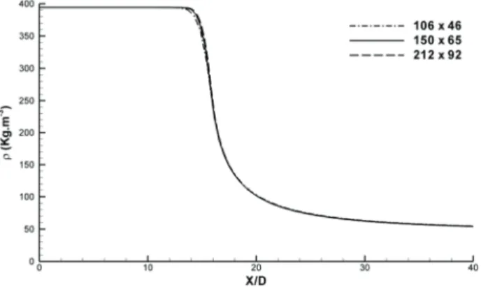
Fig. 3. Grid size dependency test based on the axial density distribution
In order to evaluate the influence of the grid on the con-verged solution grid dependency tests had to be performed.
Figure 3 shows the grid dependency test, the used grid, of 150x65 points is compared with a more refined grid of 212x92 points and with a coarser grid of 106x46 points. The results used for comparison are the axial density varia-tion in the centreline and its visible the independence of the solution from the grid size.
3. Results and discussion
Numerical results obtained in the present work are pre-sented in this section and compared with the experimental data of Mayer et al. [9], the large eddy simulations of Schmitt et al. [19] and of Jarczyk and Pfitzner [23], and also with the results obtained using the unmodified ap-proach [30, 32]. A discussion is also provided in order to reach the conclusions exposed in the next section.
Fig. 4 and 5 show the density field and streamlines for respectively the transcritical case and the supercritical case, in both figures image a) shows the results obtained while employing the Soave-Redlich-Kwong equation of state while image b) expresses the results achieved with the Peng-Robinson equation. Analysing Fig. 5 the most evident conclusion that can be taken is the appearance of a recircu-lation downstream of the injector, it is also evident the existence of entrainment of the chamber fluid into the injec-tion fluid right after the injector. This jet structure is not affected by the choice of equation of state, both Fig.5 a) and b) show exactly the same jet structure. Comparing the re-sults from both equations of state can be concluded that the Peng-Robinson equations produces higher values of density at the inlet, this is a result which could be anticipated by the results obtained in Fig. 2. It is also visible a longer potential core and deeper penetration of the jet into the chamber in the model with uses the PR equation. This can possibly be explained by the fact that the higher density at inlet causes a larger momentum, since velocity is the same, and this larger momentum takes longer to be dissipated. The supercritical case is represented in Fig. 6. A very similar jet structure is observed for this case when compared with transcritical injection conditions. There’s also the appearance of en-trainment close to the injector, and, further downstream, the existence of a recirculation. Comparing with Fig. 5 the potential core length and jet penetration is shorter for both equations of state. Like in the transcritical case also the Peng-Robinson equations of state produces higher values of density in the inlets which leads to a longer potential core.
Fig. 6 and 7 represent in better detail the evolution of density in the centreline of the jet. In Fig. 6 the axial densi-ty distribution for the transcritical case is shown for the current approach with both equations of state, these results are here compared with the experimental results from May-er et al. [9] as well as with the results obtained with the previous approach, which obtained density from Amagat’s law, and with two large eddy simulations of Schmitt et al. [19] and of Jarczyk and Pfitzner [23]. Both results of the different equations of state for the current approach show a much larger potential core than the one observed in the results of the other authors. With the Soave-Redlich-Kwong equation of state is obtained a potential core of 15.7 injector diameters, as for the Peng-Robinson equation a potential core of 16.4 injector diameters is obtained. For the same case Schmitt et al. reaches a potential core of 7.9 diameters while
Modeling of transcritical and supercritical nitrogen jets
Jarczyk and Pfitzner achieves a potential core with a length of around 9 diameters. These values of potential core length are also longer than the potential core of 11.8 obtained by the initial approach with Amagat’s law. Further downstream the current approach keeps the difficulty in fitting the experi-mental data or the other LES investigations.
a)
b)
Fig. 4. Density field and streamlines for transcritical case, a) SRK EoS, b) PR EoS
a)
b)
Fig. 5. Density field and streamlines for supercritical case, a) SRK EoS, b) PR EoS
Fig. 6. Axial density distribution for transcritical case
Fig. 7. Axial density distribution for supercritical case
The axial density distribution for the supercritical case is represented in Fig. 7. Again, the current approach employing the two different equations of state is compared with experi-mental and LES data as well as with the results obtained by the previous approach [30]. For the supercritical case a closer agreement with experimental data is obtained but the over prediction of the potential core length still exists. When using the Soave-Redlich-Kwong equation a potential core with a length of 9.4 injector diameters is observed, with the Peng-Robinson equation it increases to a length of 9.6 injector diameters. For the same test case the previous approach achieved a potential core length of 7.8 diameters, Schmitt et al. reached 5.1 while Jarczyk and Pfitzner predicted a poten-tial core with a length of 6.0 injector diameters, it’s important to refers that when analyzing the experimental results for this case the existence of a potential core is not evident. Down-stream of the potential core is obtained a better agreement with experiments between 10 and 15 diameters but then there is a departure from the data provided by Mayer [9]. Still, for this condition, the LES from Schmitt et al. [19] is not able to provide superior agreement, while the previous approach provides a closer agreement. For this case is the large eddy simulation of Jarczyk and Pfitzner which provides the closest agreement.
The full width of half maximum of density is expressed for the transcritical and supercritical test cases respectively in Figures 8 and 9. In figure 8 are represented the values obtained by the previous and current approach as well as the experimental data provided by Mayer et al. [9]. Analyz-ing first the data from Mayer, it can be seen that initially the jet appears to have a radius of twice the radius of injector,
Modeling of transcritical and supercritical nitrogen jets
this is explained in the paper of Mayer [9] by the difficulty of the technique of Raman Scattering to provide accurate values of density when the values are high. There’s then a decrease of the jet thickness until 10 x/D followed then by the expected expansion of the jet width. Similar evolution is observed by all the approaches presented in the present paper. However, when using the real fluid equations of state the potential core is longer thus delaying the expansion of the jet. In figure 12 only the results obtained by previous and current approach are exhibit since Mayer didn’t provide results for this case. Nevertheless, the evolution of the full with of half maximum of density follows the same shape obtained for the transcritical case, with the previous ap-proach showing wider expansion of jet.
Fig. 8. Axial density distribution for transcritical case
From the results of the full width of half maximum of density, it can be obtained the tangent by linear interpola-tion which represents the jet expansion rate. The linear interpolation was performed by other authors between x/D = 15 and x/D = 25. In the present work these were generally the points chosen for the calculation, however as it is visi-ble, for the current approach at transcritical conditions, the jet expansion starts only after x/D = 15, thus, for this situa-tion the interpolasitua-tion was performed between x/D = 20 and x/D = 30. These results are expressed in Table 2.
Fig. 9. Axial density distribution for supercritical case
For the transcritical case the experimental data of Mayer et al. [9] reached to a spreading rate of 0.196, a similar spreading rate was obtained by the experimental work of Oschwald and Micci [8]. The original approach used in the present investigation, for the same case predicted a
spread-ing rate of 0.316 which is an over prediction of around 61% when compared with the data of Mayer. By the introduction of a real fluid equation of state a closer agreement for the spreading rate was reached, with values of 0.250 for the SRK equation and 0.266 with the PR equation of state, representing respectively a variation of 27.6% and 35.7% when compared with Mayer’s work. The large eddy simula-tion of Schmitt et al. provides a spreading rate of 0.227 which is still closer to experimental data.
Table 2. Results of jet spreading rate
Case First Approach Amagat’s law Current
Approach Mayer et al. 2003 [9] Schmitt et al. 2009 [19] Oschwald and Micci 2002 [8] SRK PR Trans-critical 0.316 0.250 0.266 0.196 0.227 0.206 Super-critical 0.310 0.214 0.234 – 0.241 0.312
For the supercritical case Mayer et al. didn’t provide re-sults of the FWHM of Density thus not allowing the com-parison of jet spreading angle. On the other hand Oschwald and Micci [8] as well as Schmitt et al. [19] did provide results allowing a comparison to be established. The results obtained from the first approach which makes use of Ama-gat’s law replicate almost perfectly the jet spreading rate obtained by Oschwald and Micci [8]. Achieving a much better result that any of other predictions. The large eddy simulation of Schmitt et al. [19] provides an acceptable results as well, closely followed by the second approach when employing the Peng-Robinson equation of state and finally the furthest agreement comes from the second ap-proach when employing the SRK equation of state.
4. Conclusions
With the objective of testing and developing new meth-odologies to model jets at conditions around the critical point, a methodology originally developed for the study of turbulent, variable density, isothermal jets was modified to include the effects of heat transfer and a real fluid equation of state. The effects of the variation of physical properties of fluid such as thermal conductivity, specific heat at costant pressure and molecular viscosity experienced with the varia-tion of pressure and temperature were also included. To do so, in the present approach were introduced linear functions taken from the data provided by the Gas Encyclopaedia [36].
The original approach had already along this investiga-tion proved his potential for the study of this kind of fluids, despite its simplicity and inexpensive computational re-quirements. It proved to provide good agreement with ex-perimental data for supercritical injection conditions out-performing much more expensive large eddy simulations. However, it starts facing difficulties when dealing with flows in subcritical and transcritical conditions. By not accommodating the heat transfer and real fluid thermody-namics it fails to predict the correct behaviour of fluids in the transition to the two phase flow. The new approach intends overcome these lacks by the introduction of the Favre averaged energy equation and a real fluid equation of
Modeling of transcritical and supercritical nitrogen jets
state in the form of a Soave-Redlich-Kwong and a Peng-Robinson equations of state.
This new modified approach was able to improve the spreading angle results over the original approach under transcritical regime of injection, reaching a much closer agreement. The performance of the agreement at supercriti-cal conditions unfortunately suffered a decrease.
Two different reasons could be pointed out to the de-crease of accuracy at supercritical conditions. On one hand the data provided in Gas Encyclopaedia doesn’t contain values of the properties in the critical point. The critical point represents a thermodynamic singularity, thus, the properties values at this point suffer a very pronounced variation which is not accessed by the present approach. On the other hand, the flow appears to be governed by the turbulent characteristics. The ratio between turbulent
vis-cosity and turbulent thermal diffusivity is prone to suffer variations along the flow. Thus, the employment of a con-stant turbulent Prandtl number, bcd, may in fact not be the most efficient option. Future work will address these two points, expecting to obtain increased performance.
Acknowledgments
The present work has been performed under the scope of the activities of Aeronautics and Astronautics Research Center of the Associated Laboratory in Energy Transports and Aeronautics (AeroG-LAETA), UID/EMS/50022/2013.
The first authors would like to thanks to the Fundação para a Ciência e a Tecnologia (FCT), the Portuguese public agency for science and technology for the PhD scholarship SFRH/BD/87822/2012 .
Nomenclature
a, b real fluid equation of state coefficients c9 specific heat at constant pressure
C/ coefficient in turbulence model
D injector diameter [m]
ε dissipation rate of turbulent energy f mixture fraction
F mean mixture fraction i axial direction index j radial direction index k turbulent kinetic energy μ molecular viscosity μ turbulent viscosity ϕ generalized variable
ω chamber-to-injected fluid density ratio Pjk critical pressure [MPa]
Pl chamber ambient pressure [MPa]
Pk reduced presure (Pl⁄ ) Pjk
Pr Prandtl number
Pr turbulent Prandtl number ρ density [kgm–3]
ρn injected fluid density [kgm–3]
ρl injection chamber’s fluid density [kgm–3]
r radial coordinate [m] R universal constant of gases
R D⁄ radial distance normalized by injector diameter Ro$p] injector radius [m]
Rq Reynolds number
S7 source term
t time [s] T temperature [K] u axial velocity [ms–1]
U mean axial velocity [ms–1]
U$s injection axial velocity [ms–1]
v radial velocity [ms–1]
v turbulent kinematic viscosity V mean radial velocity [ms–1]
V] molar volume
X axial coordinate [m]
x D⁄ axial distance normalized by injector diameter
Bibliography
[1] BELLAN, J. Supercritical (and subcritical) fluid behavior and modeling: drops, streams, shear and mixing layers, jets and sprays. Prog. Energy Combust. Sci. 2000, 26, 329-366. [2] LACAZE, G., OEFELEIN, J.C. A non-premixed
combus-tion model based on flame structure analysis at supercritical pressures. Combust. Flame. 2012, 159, 2087-2103.
[3] NEWMAN, J.A., BRZUSTOWSKI T.A. Behavior of a liquid jet near the thermodynamic critical region. AIAA J. 1971, 9, 1595-1602.
[4] MAYER, W.O.H. et al. Atomization and breakup of cryo-genic propellants under high-pressure subcritical and super-critical conditions. J. Propuls. Power. 1998, 14(5), 835-842. [5] OSCHWALD, M., SCHIK, A. Supercritical nitrogen free jet
investigated by spontaneous Raman scattering. Exp. Fluids. 1999, 27, 497-506.
[6] CHEHROUDI, B., COHN, R., TALLEY, D. Gas behaviour of cryogenic fluids under sub- and supercritical conditions. Eighth International Conference on Liquid Atomization &
Sprays Systems. ICLASS-2000, 2000.
[7] CHEHROUDI, B., COHN, R., TALLEY, D. Spray/gas behaviour of cryogenic fluids under sub- and supercritical conditions. Eighth International Conference on Liquid At-omization & Sprays Systems. ICLASS-2000, 2000.
[8] OSCHWALD, M., MICCI, M.M. Spreading angle and centerline variation of density of supercritical nitrogen jets.
Sprays. 2002, 12(1-3), 91-106.
[9] MAYER, W., TELAAR, J., BRANAM, R. et al. Raman measurements of cryogenic injection at supercritical pres-sure. Heat Mass Transf. 2003, 39, 709-719.
[10] OSCHWALD, M. et al. Injection of fluids into supercritical environments. Combust. Sci. Technol. 2006, 178, 908038079, 49-100.
[11] STAR A.M., EDWARDS J.R., LIN K.-C. et al. Numerical simulation of injection of supercritical ethylene into nitro-gen. J. Propuls. Power. 2006, 22(4), 809-819.
[12] MARTÍNEZ-MARTÍNEZ, S., SÁNCHEZ-CRUZ, F.A., RIESCO-ÁVILA, J.M. et al. Liquid penetration length in direct diesel fuel injection. Appl. Therm. Eng. 2008, 28, 1756-1762.
Modeling of transcritical and supercritical nitrogen jets
[13] SEGAL, C., POLIKHOV, S.A. Subcritical to supercritical mixing. Phys. Fluids. 2008, 20, 1-7.
[14] SCHMITT, T., RODRIGUEZ, J., LEYVA, I.A., CANDEL, S. Experiments and numerical simulation of mixing under supercritical conditions. Phys. Fluids. 2012, 24.
[15] BARATA, J.M.M., SILVA, A.R.R., GOKALP, I. Numerical study of cryogenic jets under supercritical conditions.
Jour-nal of Propulsion and Power. 2003, 19, 142-147.
[16] ZONG, N., MENG, H., HSIEH, S.Y., YANG, V. A numeri-cal study of cryogenic fluid injection and mixing under su-percritical conditions. Phys. Fluids. 2004, 16, 4248-4261. [17] ZONG, N., YANG, V. Cryogenic fluid jets and mixing
layers in transcritical and supercritical environments. Com-bust. Sci. Technol. 2006, 178, 908038079, 193-227. [18] AOUISSI, M., BOUNIF, A., BENSAYAH, K. Scalar
turbu-lence model investigation with variable turbulent Prandtl number in heated jets and diffusion flames. Heat Mass Transf. und Stoffuebertragung. 2008, 44, 9, 1065–1077. [19] SCHMITT, T., SELLE, L., CUENOT, B., POINSOT, T.
Large-eddy simulation of transcritical flows. Comptes
Ren-dus - Mec. 2009, 337(6-7), 528-538.
[20] KIM, T., KIM, Y., KIM, S.K. Numerical study of cryogenic liquid nitrogen jets at supercritical pressures. J. Supercrit.
Fluids. 2011, 56(2), 152-163.
[21] ZHOU, L., XIE, M.-Z., JIA, M., SHI, J.-R. Large eddy simulation of fuel injection and mixing process in a diesel engine. Acta Mech. Sin. 2011, 27, 519-530.
[22] NEGRO, S., BIANCHI, G.M. Superheated fuel injection modeling: An engineering approach. Int. J. Therm. Sci. 2011, 50(8), 1460-1471.
[23] JARCZYK, M., PFITZNER, M. Large eddy simulation of supercritical nitrogen jets. 50th AIAA Aerospace Sciences
Meeting Including the New Horizons Forum and Aerospace Exposition. 2012, 1, 1-13.
[24] TERASHIMA, H., KOSHI, M. Approach for simulating gas-liquid-like flows under supercritical pressures using a high-order central differencing scheme. J. Comput. Phys. 2012, 231(20), 6907-6923.
[25] TERASHIMA, H., KOSHI, M. Strategy for simulating supercritical cryogenic jets using high-order schemes.
Com-put. Fluids. 2013, 85, 39-46.
[26] PARK, T.S. LES and RANS simulations of cryogenic liquid nitrogen jets. J. Supercrit. Fluids. 2012, 72, 232-247. [27] Schuler, M.J., Rothenfluh, T., Von Rohr, P.R. Simulation of
the thermal field of submerged supercritical water jets at near-critical pressures. J. Supercrit. Fluids. 2013, 75, 128-137.
[28] PETIT, X., RIBERT, G., LARTIGUE, G., DOMINGO, P. Large-eddy simulation of supercritical fluid injection. J.
Su-percrit. Fluids. 2013, 84, 61-73.
[29] ANTUNES, E., SILVA, A.R.R., BARATA, J.M.M. Evalua-tion of numerical variable density approach to cryogenic jets. 50th AIAA Aerospace Sciences Meeting Including the
New Horizons Forum and Aerospace Exposition. 2012, 1, 1-14.
[30] ANTUNES, E., SILVA, A., BARATA, J. RANS modeling of transcritical and supercritical nitrogen jets. 53rd AIAA
Aerospace Sciences Meeting. 2015, 1, 1-14.
[31] CHEHROUDI, B., COHN, R., TALLEY, D. Cryogenic shear layers: Experiments and phenomenological modeling of the initial growth rate under subcritical and supercritical conditions. Int. J. Heat Fluid Flow. 2002, 23, 554-563. [32] ANTUNES E., SILVA A., BARATA J. Variable density
approach for modeling of transcritical and supercritical jets.
J. Eng. Appl. Sci. 2017.
[33] SANDERS, J.P.H., SARH, B., GÖKALP, I. Variable densi-ty effects in axisymmetric isothermal turbulent jets: a com-parison between a first- and a second-order turbulence mod-el. Int. J. Heat Mass Transf. 1997, 40, 823-842.
[34] SOAVE, G. Equilibrium constants from a modified Redlich-Kwong equation of state. Chem. Eng. Sci. 1972, 27(6), 1197-1203.
[35] PENG, D.-Y., ROBINSON, D.B. A new two-constant equa-tion. Ind. Eng. Chem. Fundam. 1976, 15(1), 59-64.
[36] MEDARD L. Gas encyclopaedia, 1st ed. Amsterdam:
Else-vier Science, 1976.
Eduardo Antunes, MEng. – Aeronautical Engineer-ing at University of Beira Interior.
e-mail: EduardoFariasAntunes@hotmail.com
Prof. Jorge Barata, Habilitation – Aerospace Science Department at University of Beira Interior.
e-mail: JBarata@ubi.pt
André Silva, PhD. – Aerospace Science Department at University of Beira Interior.