Development of computational methods for the determination of biomass composition and evaluation of its impact in genome-scale models predictions

0

Universidade do Minho

Escola de Engenharia

Sophia Torres Santos

DEVELOPMENT OF COMPUTATIONAL METHODS FOR THE

DETERMINATION OF BIOMASS COMPOSITION AND EVALUATION OF

ITS IMPACT IN GENOME-SCALE MODELS PREDICTIONS.

1

Universidade do Minho

Escola de Engenharia

Sophia Torres Santos

DEVELOPMENT OF COMPUTATIONAL METHODS FOR THE

DETERMINATION OF BIOMASS COMPOSITION AND EVALUATION OF

ITS IMPACT IN GENOME-SCALE MODELS PREDICTIONS.

Dissertação de Mestrado

Mestrado em Bioinformática

Trabalho realizado sob orientação de

Professora Doutora Isabel Rocha

i

ACKNOWLEDGEMENTS

Neste momento não posso deixar de agradecer a todos os que tornaram este trabalho possível. À Professora Doutora Isabel Rocha, minha orientadora, pelos conhecimentos científicos transmitidos, pela sua constante disponibilidade e acompanhamento, pelo incentivo, motivação e confiança depositada.

À Daniela pela disponibilidade e ensinamentos, por toda a ajuda prestada, pelas longas horas de trabalho, por todo o apoio dado nos momentos bons e os menos bons, pelas gargalhadas, pelas conversas sérias, e pela grande amizade conquistada.

Ao Óscar, ao Paulo, ao Rui, à Carla e ao João que sempre estiveram disponíveis para ajudar quando precisei.

A todos os elementos do grupo BisBII, que me ajudaram a crescer a todos os níveis.

A todos os meus amigos, aqueles que sempre estiveram a meu lado, por todo o apoio dado nos momentos em que mais precisei.

À minha mãe, a quem devo todos os meus valores e educação, por sempre me encorajar a fazer melhor, a ser melhor.

Ao Dinho, por me tornar a pessoa que sou hoje, por nunca me deixar desistir dos meus sonhos, por me conhecer como ninguém. Pela motivação, confiança e paciência. E principalmente pela sua dedicação, carinho e amor.

Muito obrigada!

This work was supported in part by the ERDF—European Regional Development Fund through the COMPETE Programme (operational programme for competitiveness), and National Funds through the FCT within the project FCOMP-01-0124-FEDER-009707 (HeliSysBio—molecular Systems Biology in Helicobacter pylori).

ii DEVELOPMENT OF COMPUTATIONAL METHODS FOR THE DETERMINATION OF BIOMASS COMPOSITION AND EVALUATION OF ITS IMPACT IN GENOME-SCALE MODELS PREDICTIONS.

ABSTRACT

The use of genome-scale metabolic models is rapidly increasing in fields such as metabolic engineering. An important part of a metabolic model is the biomass equation, since this reaction will be used as the objective function in most simulation approaches. In order to obtain a reliable metabolic model, the biomass precursors and their coefficients must be as precise as possible. Ideally, the determination of the biomass composition would be performed experimentally, but due to technical limitations in cellular components quantification, budget restraints and time limitations, this is often established by approximation to closely related organisms. Computational methods however, can extract some information from the genome, such as amino acid and nucleotide compositions.

One main objective in this study was to evaluate how biomass precursor coefficients computationally determined, affected the predictability of several genome-scale metabolic models by comparison with experimental data. Sensitivity analysis studies were performed with the Escherichia coli iAF1260 metabolic model concerning specific growth rate and flux distribution. Several metabolic models, whose biomass composition had been experimentally determined, were used to evaluate the impact of biomass coefficients on growth rates and flux distributions. In this study, biomass precursor coefficients were changed based on data obtained from computational methods and from closely related organisms. The results obtained from these two changes were then compared to the results obtained from the model using the experimentally determined biomass composition. Finally, analytical methods were established for macromolecule quantification and protein, DNA and RNA content of Helicobacter pylori biomass were experimentally determined.

The results obtained suggest that small modifications (around 1×10-2) in biomass precursor coefficients have no significant impact on the computed specific growth rate and flux distributions. We also observed that, despite computationally determined biomass coefficients present differences to those experimentally determined, the growth rate and flux distributions have similar results (differences below 1,5 %). Surprisingly, specific growth rates and flux distributions were more distant from experimental data when adopting biomass precursor coefficients from closely related organisms.

Keywords: Genome-scale metabolic models, computational methods, experimental determination, biomass composition.

iii DESENVOLVIMENTO DE MÉTODOS COMPUTACIONAIS PARA A DETERMINAÇÃO DA COMPOSIÇÃO DA

BIOMASSA E AVALIAÇÃO DO SEU IMPACTO EM PREVISÕES DE MODELOS À ESCALA GENÓMICA

RESUMO

O uso de modelos metabólicos à escala genómica tem grande importância áreas, tais como a engenharia metabólica. A equação da biomassa é uma das reações fundamentais nestes modelos, uma vez que esta reacção é usada como função objectivo na maioria das abordagens de simulação. Para se obter um modelo à escala genómica coerente, os percursores da biomassa devem ser o mais precisos possível. A composição da biomassa deveria ser determinada experimentalmente; contudo, devido a limitações técnicas de quantificação, limitações de material biológico e tempo, muitos modelos metabólicos adoptam a composição da biomassa de organismos similares. No entanto, alguns métodos computacionais conseguem estimar coeficientes de aminoácidos e nucleótidos, a partir de informação do genoma.

Neste trabalho, pretende-se avaliar o impacto que os coeficientes estimados a partir da informação do genoma, têm na previsão destes modelos à escala genómica, comparando-os com dados experimentais. Realizou-se uma análise de sensibilidade aos coeficientes da composição da biomassa do modelo à escala genómica da Escherichia coli iAF1260, comparando valores de taxa específica de crescimento e distribuição de fluxos. Foram também usados outros modelos à escala genómica, que possuem composição da biomassa com dados experimentais, de modo a avaliar o impacto da alteração da composição da biomassa na taxa específica de crescimento e distribuição de fluxos. Neste estudo fez-se a alteração da composição da biomassa com valores estimados in silico e com valores experimentais de organismos similares. Os valores de taxa específica de crescimento e de distribuição de fluxos obtidos para cada composição de biomassa foram comparados com os respectivos valores da composição da biomassa experimental. Por fim, procedeu-se também à implementação de métodos para análise da composição da biomassa em macromoléculas e determinou-se experimentalmente a composição de proteína, DNA e RNA total para o organismo Helicobacter pylori.

Os resultados obtidos sugerem que pequenas alterações (na ordem de 1×10-2) nos coeficientes da composição da biomassa não afectam os valores das taxas específicas de crescimento e distribuição de fluxos. Observa-se também que os coeficientes da biomassa estimados a partir da composição do genoma, apesar de não serem muito semelhantes aos determinados experimentalmente, produzem resultados de taxa específica de crescimento e distribuição de fluxos muito semelhantes (diferenças menores que 1,5%). Estas diferenças são menores do que quando se adopta composições de biomassa de organismos semelhantes.

Palavras-chave: Modelos metabólicos à escala genómica, métodos computacionais, métodos experimentais, composição da biomassa.

iv

INDEX

INDEX OF FIGURES ... VIII

INDEX OF TABLES...IX

1 BACKGROUND... 1

1.1 SYSTEMS BIOLOGY ... 1

1.2 GENOME-SCALE METABOLIC RECONSTRUCTIONS ... 1

1.3 FLUX BALANCE ANALYSIS ... 2

1.4 BIOMASS OBJECTIVE FUNCTION ... 3

1.4.1 Experimental determination of biomass composition ... 4

1.4.2 In silico determination of biomass composition ... 6

2 MATERIAL AND METHODS ... 9

2.1 EXPERIMENTAL BIOMASS DETERMINATION ... 9

2.1.1 Strains and Cultivation conditions ... 9

2.1.2 Biomass macromolecular content determination ... 9

2.2 IN SILICO BIOMASS ANALYSIS ... 10

2.2.1 Biomass Amino Acids and Nucleotides compositions ... 10

2.2.2 In silico Simulations ... 11

3 RESULTS AND DISCUSSION ... 14

3.1 BIOMASS COMPOSITION IN EXISTING MODELS... 14

3.2 EXPERIMENTAL BIOMASS DETERMINATION ... 16

3.2.1 Macromolecular composition... 16

3.3 IN SILICO BIOMASS COEFFICIENTS ESTIMATION ... 16

3.4 IN SILICO SIMULATIONS ... 19

3.4.1 Sensitivity analysis ... 19

3.4.2 Impact of Biomass composition in specific growth rate predictions ... 22

v

4 CONCLUSIONS AND FUTURE WORK ... 28

4.1 CONCLUSIONS ... 28

4.2 FUTURE WORK ... 29

5 REFERENCES ... 30

vi

ABBEVIATURES

Bsu Bacillus subtilis

ca2 Calcium cl Chloride coa Coenzyme A cobalt2 Co2+ ctp CTP cu2 Cu2+ cys-L L-Cysteine

DAPI 4,6-diamidino-2-phenylindole dihydrochloride

datp dATP

dctp dCTP

dgtp dGTP

dttp dTTP

FBA Flux balance analysis

fad Flavin adenine dinucleotide oxidized

fe Fe2+ fe3 Fe3+ gln-L L-Glutamine glu-L L-Glutamate gly Glycine gtp GTP his-L L-Histidine ile-L L-Isoleucine k potassium

kdo2lipid4 KDO(2)-lipid IV(A)

leu-L L-Leucine

vii Lpl Lactobacillus plantarum lys-L L-Lysine met-L L-Methionine mg2 Magnesium mlthf 5,10-Methylenetetrahydrofolate mn2 Mn2+ mobd Molybdate

murein5px4p two disacharide linked murein units nad Nicotinamide adenine dinucleotide

nadp Nicotinamide adenine dinucleotide phosphate

nh4 Ammonium

pe160 Phosphatidylethanolamine (dihexadecanoyl, n-C16:0) pe161 Phosphatidylethanolamine (dihexadec-9enoyl, n-C16:1) pFBA Pasimonius flux balance analysis

phe-L L-Phenylalanine

pheme Protoheme

pi Phosphate

Ppu Pseudomonas putida

pro-L L-Proline

pydx5p Pyridoxal 5'-phosphate

ribflv Riboflavin

ser-L L-Serine

sheme2 Siroheme

so4 Sulfate

Sty Salmonella typhimurium

thf 5,6,7,8-Tetrahydrofolate

thmpp Thiamine diphosphate

thr-L L-Threonine

trp-L L-Tryptophan

tyr-L L-Tyrosine

udcpdp Undecaprenyl diphosphate

utp UTP

val-L L-Valine

Vvu Vibrio vulnificus

viii

INDEX OF FIGURES

Figure 1. Flow chart to calculate the fractional contribution of a percursor to the biomass reaction (Adapted from Thiele et al., 2010) ... 8 Figure 2. Chart indicating the origin of the data incorporated in the biomass equations in the genome-scale metabolic reconstructions reviewed. ...14 Figure 3. Differences for growth rate predictions between using experimental and in silico biomass composition for each organism studied, represented in percentage. AA represents amino acids coefficients, dNTPs represents deoxynucleotides coefficients, NTPs represents nucleotides coefficients and All represents simultaneous changes in amino acids, deoxynucleotides and nucleotides coefficients. ...23 Figure 4. Differences for the specific growth rates predictions between experimentally determined biomass composition and three other setups: using in silico building blocks composition together with experimental macromolecular composition for the studied organism (IS), original (experimental) building blocks composition and E. coli macromolecular composition (E. coli) and original (Experimental) building blocks composition and B. subtilis macromolecular composition (B. subtlis). ...24 Figure 5. Differences for the specific growth rates predictions between experimentally determined biomass composition and three other setups: using in silico building blocks composition together with experimental macromolecular composition for the studied organism (IS), building blocks and macromolecular composition from E. coli (E. coli) and building blocks and macromolecular composition from B. subtilis (B. subtlis) ...25 Figure 6. Sum of squared differences between flux distributions obtained with experimental values and three setups: in silico building blocks compositions (with original macromolecular composition); E. coli macromolecular and building blocks composition and B. subtilis macromolecular and building blocks composition. ...27

ix

INDEX OF TABLES

Table 1. Organisms with metabolic models used in in silico simulations ...11 Table 2. Table summarizing the origin of the biomass composition data in genome-scale metabolic reconstructions for which at least part of the composition has been experimentally determined. ...15 Table 3. Experimental values of the macromolecular components Protein, DNA and RNA. ...16 Table 4. Differences between macromolecular composition of gram-negative organisms and E. coli. ...17 Table 5. Differences between macromolecular composition of gram-positive organisms and B. subtilis. 17 Table 6. Average, maximum and minimum differences, between in vivo and in silico data, for amino acids, deoxynucleotides and nucleotides. ...18 Table 7. Sensitivity analysis of macromolecular coefficients variation for sensitivity factors of 10% and 50%. Nominal composition is given in parentheses. ...20 Table 8. Sensitivity analysis of the building blocks coefficients variation (top 20) for a sensitivity factor of 50%. ...21 Table 9. Jaccard Differences, of flux distributions, between experimental and altered biomass compositions with in silico , E. coli and B. subtilis coefficients. ...26 Table A 1. Macromolecular compositions and in vivo and in silico building blocks compositions for all organisms with experimental data available. ...34 Table A 2. Table representing the sensitivity analysis of each macromolecular and building block component. ...36 Table A 3. Specific growth rate for experimental and altered biomass compostions. ...50 Table A 4. Differences in specific growth rates between experimental and altered biomass compositions. ...51 Table A 5. Sum Squared Differences, of flux distribution, between experimental and altered biomass compositions. ...52 Table A 6. Jaccard Differences, of flux distributions, between experimental and altered biomass compositions. ...53

1

1 B

1.1 Systems Biology

The huge development of molecular biology was the basis to the appearance of the tools known as omics – genomics, transcriptomics, proteomics, metabolomics, interactomics, fluxomics, etc. Despite the large amount of data that these approaches create every day, living systems are to complex being thus difficult to predict their behavior over time and under various conditions. Systems biology is an

emerging, interdisciplinary and integrated study of complex interactions on all omics levels of biological systems. The aim of systems biology is to understand biological systems, studying their structure, dynamics, control and design methods (Kitano, 2002), by integrating computational and theoretical approaches with experimentalefforts. New knowledge in this field is being gathered through tools such as automated genome annotation, genome-scale metabolic reconstructions and regulatory network reconstructions using microarray data (Edwards et al, 2002).

1.2 Genome-scale metabolic reconstructions

Nowadays, an indispensable tool for the study of metabolic systems biology is the genome-scale metabolic network reconstruction (Thiele et al, 2010). The first metabolic network reconstruction was published in 1999 (Edwards et al, 1999) and they are becoming available for an increasing number of organisms each year (Gianchandani et al, 2010). These network reconstructions represent the majority of the metabolic reactions in an organism and the genes that encode each enzyme, integrating mathematical models and biochemical data. They are used to compute a variety of phenotypic states (Feist et al, 2010) of an organism under different environmental and genetic conditions (Rocha et al., 2008). Some effective applications of constraint-based analyses of reconstructed metabolic networks are associated to metabolic engineering strategies, prediction of outcomes of gene deletions, drug-target identification, etc (Chandra et al, 2009). Thus a genome-scale metabolic reconstruction is of huge importance but is an arduous and time-consuming work, as demonstrated by Thiele and Palsson, that in 2010 published a detailed protocol, with 96 steps, to create a genome-scale metabolic model reconstruction. Some of the essential steps are, for example, genome annotation, reactions identification and stoichiometry determination, compartmentation, determination of the biomass composition, energy requirements and additional constraints (Rocha et al., 2008).

2 Nowadays there are tools to create a genome-scale metabolic reconstruction. The most well-known is The SEED, a web-based resource that provides in approximately 48 hours, a genome-scale metabolic model from an assembled genome sequence of prokaryotic organisms (Henry et al., 2010). The outputted metabolic model becomes free to the public and everyone can reach it and extract knowledge.

1.3 Flux balance analysis

Flux balance analysis (FBA) is a widely used approach for the genome-scale determination of metabolic fluxes at steady-state conditions. An FBA formulation determines the flow of metabolites through a metabolic network, making possible to predict the growth rates, substrate uptake rates, and product secretion rates of an organism (Feist et al, 2010). FBA has a high range of applications, such as optimization of bio-processes in industries, identification of drug targets and an improved annotation of genomes (Chandra et al., 2009).

FBA uses linear optimization to determine the steady-state reaction flux distribution in a metabolic network. The metabolic network can be represented by a stoichiometric matrix , of dimensions m x n, where m corresponds to the total number of metabolites and n to the total number of reactions in the network. The coefficients of the matrix define the relationship between the reactions and compounds of the metabolic network. An optimal solution consistent with the known constraints and with respect to the maximization or minimization of some objective function ( ) can be obtained by solving the linear problem:

where is a vector of fluxes of each reaction and and are the lower and upper limits for the fluxes, respectively. These limits are used to model irreversible reactions, to limit uptake and secretion rates and to specify measured fluxes (Rocha et al., 2008).

The major challenge in FBA is the definition of an objective function with biological relevance (Gianchandani et al., 2010). A variety of objective functions have been used in order to define an FBA

3 problem. However, several studies in different organisms demonstrated that the organism evolves towards to the maximization of the specific growth rate (Rocha et al., 2008).

1.4 Biomass objective function

The most common objective function involves the maximization of biomass, which allows for a wide range of predictions, consistent with experimental observations, although, under some conditions, the behavior of cellular systems is incompatible with biomass maximization (Chandra et al, 2009). The formulation of the biomass objective function can be obtained at different levels of detail: basic level (define the macromolecular content on the cell, i.e., protein, RNA, DNA, lipids), intermediate level (calculate the necessary biosynthetic energy) and advanced level (detailing the necessary vitamins, elements, and cofactors) (Feist et al, 2010). If a biomass precursor is not accounted for in the biomass reaction, the synthesis reactions may not be required for growth as well as the associated genes. Thus, the composition of the biomass reaction plays an important role for example for in silico gene deletion experiments (Thiele et al, 2010).

The detailed biomass composition of an organism needs to be experimentally determined for cells growing in log phase before being included in the metabolic models. For that purpose, there are several methods available. However, in many cases that composition has not been determined and a biomass composition of related organisms is included in the model.

For n biomass constituents, the biomass equation can be formulated as:

∑

where is the coefficient of each macromolecule or building block, , considered in the biomass. The units of all the coefficients are defined in mmol per gram of dry weight (mmol/gDW) and the biomass units are defined per hour (h-1).

4 1.4.1 Experimental determination of biomass composition

A detailed biomass composition of an organism needs to be experimentally determined for cells growing in log phase. The range of different compounds that are part of a biomass equation requires the application of different analytical techniques. Some of the techniques most used to experimentally determine biomass composition are described below.

1.4.1.1 Experimental determination of Macromolecular Content

Macromolecular content usually refers to major groups of biomass constituents, as DNA, RNA, protein, carbohydrates and lipids. As it was said before, this study is focused only in protein, DNA and RNA macromolecular compositions.

Biomass total DNA content

DNA content of biomass can be determined by means of the Hoechst fluorescence dye method that is described in Mey et al, 2006. In this method, Hoechst dye is added to biomass samples in TNE buffer. Hoechst binds strongly to adenine-thymine rich regions in DNA. However, Hoechst dye can be replaced by 4',6-diamidino-2-phenylindole (DAPI), that is also a fluorescent dye specific to adenine-thymine rich regions in DNA, and it can be used instead of Hoechst in equimolar amounts (Torsvik, 2004). The fluorescence in both cases is measured using the excitation/emission wavelengths of 350nm/460nm.

It is also common the use of the diphenylamine-colorimetric method for DNA to determine the total DNA content (Burton et al., 1956), although this method is time consuming (16 - 20 hours at 30ºC) when compared with the Hoechst fluorescence dye method. It has also been reported (Mey et al, 2006) that the Hoechst fluorescence dye method is more sensitive and precise than the diphenylamine-colorimetric method.

Some authors also reported the use of DNA extraction kits (McOrist et al, 2002). These kits are available from various companies like Qiagen, Bio-Rad and Invitrogen, that supply sample and assay technologies for molecular diagnostics. These DNA extraction kits are simple to use, although they do not guarantee the total extraction of DNA from the cells.

DNA content is normally calculated by interpolation in a calibration curve performed using a standard. It is common to use calf thymus DNA as a standard. The main criterion for choosing a specific type of standard DNA is the GC content that should be similar to the GC content of the samples. For

5 instance, the GC content of salmon sperm and of calf thymus DNA is very similar, 41,2% and 41,9%, respectively.

Biomass total RNA content

RNA biomass content is mainly determined using the cold perchloric acid extraction, reported by Benthin (Benthin et al, 1991). In this method, RNA is extracted by digesting biomass with a KOH solution and collecting RNA with cold HClO4 solutions of different concentrations.

The method of a colorimetric reaction with orcinol (Endo, 1970) was also reported by some authors (Oliveira et al., 2005 and Kjeldsen et al., 2009). The method starts with a hot perchloric acid hydrolysis of DNA and RNA. The RNA composition is then determined by adding orcinol solution to the samples (Mey et al, 2006) and using a derivative of ribose. It has been reported (Benthin et al, 1991) that the cold perchoric acid extraction is more sensitive and precise than the colorimetric reaction with orcinol.

Like with DNA, some authors also reported the use of RNA extraction kits (Nuyts et al, 2001) that are supplied by companies that supply sample and assay technologies for molecular diagnostics. However, these kits are specific to extract enriched mRNA, selectively excluding RNAs that have less than 200 dNTPs, which represent 15 – 20% of total RNA.

RNA content is normally calculated by measuring the absorbance at 260 nm and multiplying the value by 44, since an absorbance of 1 unit at 260 nm corresponds to 44 µg of RNA per mL.

Biomass total protein content

Protein biomass content determination has been reported to use colorimetric methods such as the Biuret method (Dauner et al, 2001 and Novak et al., 1999), the Lowry method (Cocaign-Bousquet et al., 1995) and the Bradford method (Sohn et al., 2010b).

In the Biuret method, copper ions from an alkaline cupric sulfate solution bind to peptide nitrogens forming a complex that absorbs light at 540 nm. Copper reacts with peptide bounds limiting the reaction to free amino acids. Thus, this method is useful with samples with a high concentration of protein.

The Lowry method is the most commonly used to quantify total protein because it is very sensitive and highly reproducible. This method combines the reaction of copper ions, binding to peptide bounds like in the Biuret method and the Folin-Ciocalteu reagent that oxidizes aromatic amino acids (tryptophan and tyrosine). Thus, this method, despite being very sensitive, depends on the protein composition in aromatic amino acids.

6 The Bradford method uses the Comassie Brilliant Blue G-250 dye that forms strong non covalent complexes with proteins and, under acidic conditions, shifts the initial red form to a blue form. This method is sensitive and accurate but is linear only for low concentrations (0 - 2 mg/mL) (Nelson et al., 2008).

Protein content is normally calculated by interpolation in a calibration curve performed using bovine serum albumin (BSA) as standard.

1.4.1.2 Experimental determinations of Amino Acid composition

The first step of the determination of amino acid composition is protein hydrolysis. In general, and for all of the cases studied, the most common method used is the gas phase hydrolysis, where the biomass samples are exposed to HCl 6M at 105ºC for 24 hours. In this step the objective is to break the peptide bonds between resulting in free amino acids of the total protein, but that does not always occur. Some amino acids are very sensitive to hydrolysis, particularly cysteine, tryptophan and methionine (Fountoulakis et al., 1998), while asparagine is transformed in aspartic acid and glutamine is transformed in glutamic acid. There are several agents that can be added to HCl in order to protect these amino acids. The addition of thiaglycolic acid to the HCl solution is reported to stabilize some amino acids, such as methionine, cysteine and tryptophan (Joergensen, et al, 1995).

After hydrolysis, the separated amino acids are generally derivatized. The derivatization method most commonly used is the one that uses as derivatives o-phthaldehyde (OPA) and 9-fluoroenylmethyl-chloroformate (FMOC). OPA is added first to the sample in order to react with primary amino acids. The secondary amino acids do not react with OPA, but are then derivatized using FMOC. These derivatives are mainly analyzed by high-pressure liquid chromatography (HPLC).

1.4.2 In silico determination of biomass composition

The application of computer technology to the management of biological information is a faster and simpler way to estimate the biomass composition in amino acids, deoxynucleotides (dNTPs) and nucleotides (NTPs). Here some methods to obtain an estimation of the biomass composition from genome information will be described.

According to Thiele and co-authors (Thiele et al, 2010) the estimation of amino acid composition from genome information can be performed by calculating the percentage of each codon usage. The

7 codon usage can be obtained from files with sequences of all the genes encoding for proteins. These files with genome information are easily found in databases and can be extracted in various formats, like FASTA and GENBANK formats. Afterwards, to calculate the weight per mol of protein, it is necessary to use the molar percentage and molecular weight of each amino acid. Then the individual amino acid values are summed to give a total molecular weight of the protein content. With this value, it is possible to calculate the weight percent per amino acid. This weight percent is then multiplied by the cellular content percentage of the macromolecule and divided by the molecular weight of the individual monomer (Figure 1).

The estimation of the nucleotide composition from genome information can be determined by calculating the number of each dNTP (i.e., dATP, dCTP, dGTP, and dTTP). This number can be also found in databases. Finally, it is necessary to calculate the fractional distribution of each nucleotide in the biomass composition using the same protocol applied to calculate the amino acid fraction.

In order to determine the RNA composition of the cell, the protocol described by Thiele and Palsson uses the codon usage accessed for the amino acid content. Since RNA incorporates uracil (U) instead of thymine (T), the codon usage needs to be read with every T replaced by a U. Then, it is necessary to calculate the fractional distribution of each nucleotide to the biomass composition using the same protocol to calculate the amino acid fraction. However, in this report the authors do not distinguish between the different types of RNA and perform their calculations for mRNA only, which is particularly important since rRNA accounts for the majority of the RNA content in any cell.

A bioinformatics tool that provides an estimation of biomass composition in dNTPs, NTPs and amino acids, based in the protocol described by Thiele and Palsson (2010) has already been developed under the scope of the “Project” Curricular Unit in the first year of this Master program. The tool was implemented in the Java language and requires the input of files containing genome sequences from DNA, RNA and protein, in the FASTA format. This tool was used to estimate the biomass composition in amino acids, dNTPs and NTPs using genome information of the most detailed and complete metabolic reconstruction of an organism to date, the common laboratory strain Escherichia coli K-12 MG1655(Orth et al, 2011). In general, the results obtained were fairly close to the laboratory data of the reference used. However, there are significant differences in the biomass composition in several amino acids. These differences may probably result from the following causes: in one hand, we are comparing the results of the estimation with experimental data, which can be affected by experimental errors; on the other hand, in the in silico approach we are supposing that all proteins are expressed at the same time, in the same proportions, a fact that is known to be false.

8 Figure 1.Flow chart to calculate the fractional contribution of a percursor to the biomass reaction(Adapted from

Thiele et al., 2010)

Figure 2. Flow chart to calculate the fractional contribution of a percursor to the biomass reaction(Adapted from [2])

mmol monomer/g dry weight

e.g. Ala: (0,0663(gAla/gProtein)*0,563((gProtein/gDW)*1000(mmolAla/molAla))/89,094g/mol)=0,4190(mmolAla/gDW)

g monomer/ g macromolecule

e.g. Ala: 8,4826 (gAla/molProtein)/110,35 (gProtein/molProtein)=0,0663 (gAla/gProtein)

g monomer/mol macromolecule

e.g. Ala:0,09521(mol/mol)×(89,094g/mol)=8,4826 (gAla/molProtein)

% of monomer per genome

e.g. Ala : 0,09521 (mol/mol)

Genome Information /Experimental Data

× Molecular weight of monomer

: ∑g monomer/mol macromolecule

× % macromolecule/cell : molecular weight × 1000

Another approach used to compute the biomass composition in silico has been adopted by The SEED tool (DeJongh et al, 2005). The biomass equation is based in a template biomass reaction that includes 83 small-molecules, 39 universal building blocks (e.g. amino acids, NTPs and dNTPs), and 44 reactants based on specific criteria in the annotated genome that include cell wall type criteria: gram-positive or gram-negative.There are rules to determine the coefficients of biomass components in each organism. The values of amino acids, dNTPs, NTPs, protein, DNA, RNA and cofactors are based in the values of Escherichia coli for gram-negative organisms and Bacillus subtilis for gram-positive organisms. The coefficients of small molecules are adjusted to improve the accuracy of predicted growth yields. It is also assumed that the growth-associated ATP consumption is 60 mmol per gram of biomass per hour. All cofactors are present in equal mass (0.10/total mass of all cofactor components). The net mass of all biomass components sums to one (Henry et al., 2010).

9

2 MATERIAL AND METHODS

2.1 Experimental biomass determination

2.1.1 Strains and Cultivation conditions

In this study the strain Helicobacter pylori 26695 was used.

Helicobacter pylori strain was cultured according to Testerman et al. (2001), at 37ºC using the chemically defined medium ham’s F-12 nutrient mixture.

Culture samples of 40 mL of volume were centrifuged at 7800 rpm for 5 minutes and washed twice in 40 mL of phosphate buffered saline (PBS), pH 7,4. The samples were all dried at 60ºC until no alteration in weight was observed.

2.1.2 Biomass macromolecular content determination 2.1.2.1 Biomass total DNA content

DNA content of biomass was determined according to Mey et al. (2006) with some modifications: 4,6-diamidino-2-phenylindole dihydrochloride (DAPI) was used instead of Hoechst as the fluorescent dye solution and salmon sperm DNA was used as standard to perform a calibration curve instead of calf thymus DNA.

Dried biomass samples were dissolved in TNE buffer (0,1 M NaCl, 10 mM EDTA, 10 mM Tris, pH 7,4) at a concentration of 5 mg/mL. Then 33 µL of the sample solution was mixed with 1 mL of DAPI dye solution (DAPI 0,25 µg/mL in TNE buffer) and incubated for 30 min. Fluorescence was measured using the excitation/emission wavelengths of 350/460 in a black 96-well microtiter in a Spectrofluorimeter Jasco FP-6200. DNA content was calculated by interpolation in a calibration curve performed using as a standard salmon sperm DNA.

2.1.2.2 Biomass total RNA content

RNA content of biomass was determined according to Benthin (Benthin et al, 1991) with some modifications. Dried biomass samples, with 5 mg, were resuspended in 10 mL 0,7 M HClO4previously cooled and incubated for 5 min. After incubation, biomass was centrifuged at 7800 rpm for 12 min at

4°C. The pellet was washed twice and resuspended in 10 mL 0,3 M KOH. The resuspended biomass was then divided in two aliquots with the same volume and incubated at 37°C for 1 h. One mL of cold 3 M

10 HClO4 was added and the samples were centrifuged. The supernatant was collected and the pellet was washed twice with 1 mL 0,5 M HClO4. The three supernatants collected were mixed and absorbance was measured at 260 nm using a Micro-Spectrophotometer Nanodrop. RNA content was calculated taking into account the sample dilution.

2.1.2.3 Biomass total Protein content

Protein content was determined by using the Biuret method according to Verduyn (Verduyn et al., 1990). One milliliter of dried biomass (2 g/L) was mixed with 0,5 mL 1 M NaOH, incubated at 100°C for 10 min and subsequently cooled on ice. Then, 0,9 mL of the solution were mixed with 0,3 mL of 0,1 M copper sulfate solution and incubated for 5 min at room temperature. Ended that time, the solution was centrifuged for 5 min at 10000 rpm. The absorbance was measured at 540 nm in a 96-well microtiter plate in a Microplate reader for ELISA Bio-Tek Synergy HT. Protein concentration was calculated by interpolation in a calibration curve using bovine serum albumin (BSA) as standard.

2.2 In silico biomass analysis

2.2.1 Biomass Amino Acids and Nucleotides compositions

The estimation of amino acid, dNTPs and NTPs compositions for the biomass equation was determined from genome information and using a java tool according to the protocol published by Thiele and Palsson (Thiele et al, 2010). The java tool uses FASTA files with the sequences of interest: for amino acids composition a FASTA file with all coding sequences (FASTA Protein); for dNTPs composition a FASTA file with the complete sequence of the genome; for NTPs composition 3 FASTA files, one with rRNA sequences, one with tRNA sequences and one with the mRNA sequences (coding sequences - FASTA Nucleotide). These sequences were obtained from the NCBI database. Obligatory inputs are also needed: total macromolecular contents (protein, DNA and RNA) and mRNA, tRNA and rRNA percentages of total RNA. It was assumed that for gram-negative organisms the percentages used for mRNA, tRNA and rRNA were 5%, 15% and 80%, respectively. For gram-positive organisms the percentages used were 5%, 20% and 75%, respectively.

11 2.2.2 In silico Simulations

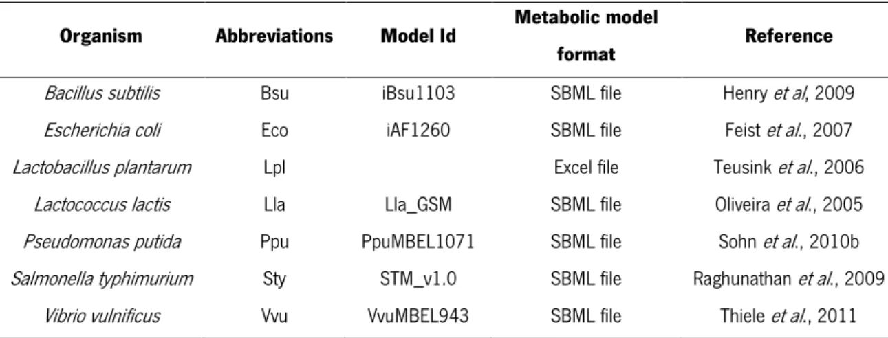
In order to evaluate the impact of the use of different coefficients in the biomass equation, in silico simulations were made. For in silico simulations, the Optflux 3.06 software tool (Rocha et al., 2010) was used. For that, 7 out of the 10 genome-scale metabolic models from bacteria that have experimentally determined biomass compositions were simulated using Optflux (Table 1). For the simulations, the parcimonious Flux Balance Analysis method was used using biomass maximization as the objective function. All simulations performed were “wild-type” as no genetic modification was introduced in the model in any simulation.

The genome-scale metabolic models used were provided in the Systems Biology Markup Language (SBML) format and in an Excel format that included a sheet with all metabolites of the model and a sheet with all reactions of the model. It was not possible to simulate the genome-scale metabolic models from Clostridium acetobutylicum, Corynebacterium glutaminicum and Mannheimia succiniciproducens using Optflux. These 3 models were published in excel files and their format was not compatible with any version of Optflux (or any other known simulation tool), not allowing their simulation.

Table 1. Organisms with metabolic models used in in silico simulations

Organism Abbreviations Model Id Metabolic model

format Reference

Bacillus subtilis Bsu iBsu1103 SBML file Henry et al, 2009

Escherichia coli Eco iAF1260 SBML file Feist et al., 2007

Lactobacillus plantarum Lpl Excel file Teusink et al., 2006

Lactococcus lactis Lla Lla_GSM SBML file Oliveira et al., 2005

Pseudomonas putida Ppu PpuMBEL1071 SBML file Sohn et al., 2010b

Salmonella typhimurium Sty STM_v1.0 SBML file Raghunathan et al., 2009

Vibrio vulnificus Vvu VvuMBEL943 SBML file Thiele et al., 2011

Some modifications were made to the model of Pseudomonas putida regarding amino acids composition. It was verified that the units used were not standardized and so they were converted to mmol/gDW.

12 2.2.2.1 Sensitivity analysis

A sensitivity analysis to the coefficients of biomass precursors was made, in order to evaluate the impact of these modifications in specific growth rate and flux distribution predictions. For that, a java tool was built that uses the Optflux 3.06 software to simulate the model once for each perturbation. For a given factor, the tool changes the coefficient of each macromolecule or building block (one at a time) and compensates all other coefficients so that the sum of all coefficients has the same value as the sum of the original values. There are some mandatory inputs: a model in the SBML format, a file with all macromolecular components and percentages, and files with each individual macromolecular constituent and its composition (e. g. a Protein file contains amino acid content, percentage and molecular weight), and one or more sensitivity factors (i.e. coefficient variation). For each sensitivity factor, a wild-type simulation was performed and the calculated specific growth rate and the flux distribution of all reactions retrieved.

2.2.2.2 Effects in the specific growth rate

Wild type simulations were made for each organism in Table 1, except for Escherichia coli, with the experimental and altered biomass compositions. The differences obtained for the specific growth rates using both compositions were expressed in percentage, according to the following expression:

(| |

)

Where Exp represents the specific growth rate obtained using the biomass composition determined experimentally and X represents the specific growth rate calculated from the biomass composition that was altered.

13 2.2.2.3 Flux distribution analysis

Wild type simulations were made for each organism in Table 1 with the experimental and altered biomass compositions. The flux values for each reaction were obtained for all cases.

The differences between the flux values obtained using experimental and altered biomass compositions were evaluated using the distance measure sum of squared differences (SSD), according to the following expression:

∑

Where x represents the flux value of a given reaction, i, in the simulation performed with experimental biomass composition and y represents the flux value of the same reaction for the altered biomass reaction. IN represents the total number of metabolic fluxes.

The flux difference was also evaluated by computing the jaccard distance that evaluates which reactions change from having zero flux to a greater than zero flux from one condition to the other, according with the following expression:

Where p represents the number of reactions with a flux in both simulations performed using the experimental and altered biomass composition models, q represents the number of reactions with flux in the experimental biomass composition model and with no flux in altered biomass compositions models and d represents the number of reactions with no flux in the experimental biomass composition model and with flux in altered biomass compositions models.

14

3 RESULTS AND DISCUSSION

3.1 Biomass Composition in existing models

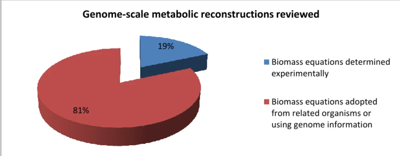
A study of 81 curated genome-scale metabolic reconstructions (Schellenberger et al, 2010) was made in order to understand how the biomass composition is currently obtained. This study focused only in the macromolecular content (protein, DNA and RNA), amino acids, dNTPs and NTPs compositions. From the analysis of the biomass equation of each model, it was verified that only 19% of the biomass equations had been, to some extent, experimentally determined while the remaining 81% were adopted from other related organisms or determined using genome information (Figure 2).

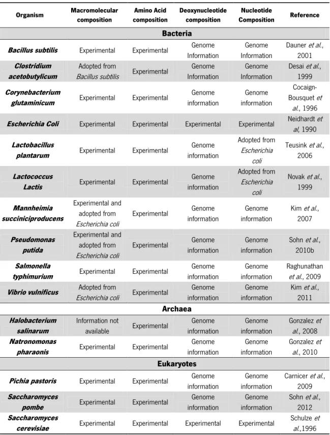
However, even for those 19% that had experimental measurements, in the vast majority (exception made for Saccharomyces cerevisiae) not all of the biomass components were experimentally determined. Some of the components are assumed to be equal to other related organisms and others were obtained using genome information (Table 2).

For 50 % of the genome-scale metabolic reconstructions of prokaryotic organisms available, even though with clear genomic, metabolic and phenotypic differences, the biomass composition adopted is the one from Escherichia coli. It should however be emphasized that the biomass composition from Escherichia coli was determined experimentally by Neidhardt (Neidhardt et al, 1996) and that, since these studies, no significant experimental data have been published for this organism. Most of the times, data from Escherichia coli is used because it has been reported that the use of a generic biomass formation reaction in FBA simulations was previously tried and led to successful predictions (Kim et al., 2010 and Ates et al., 2011). However, other authors have reported that the use of Escherichia coli’s biomass composition produce predictions that have some major differences due mainly to differences in fatty acids

19%

81%

Genome-scale metabolic reconstructions reviewed

Biomass equations determined experimentally

Biomass equations adopted from related organisms or using genome information

Figure 2. Chart indicating the origin of the data incorporated in the biomass equations in the genome-scale metabolic reconstructions reviewed.

15 and amino acid composition (Raghunathan et al., 2009). Thus, the development of an accurate biomass equation for a given organism is of huge importance in in silico simulations.

Table 2. Table summarizing the origin of the biomass composition data in genome-scale metabolic reconstructions for which at least part of the composition has been experimentally determined.

Organism Macromolecular composition Amino Acid composition Deoxynucleotide composition Nucleotide Composition Reference Bacteria

Bacillus subtilis Experimental Experimental Genome

Information Genome Information Dauner et al., 2001 Clostridium acetobutylicum Adopted from

Bacillus subtilis Experimental

Genome Information Genome Information Desai et al., 1999 Corynebacterium

glutaminicum Experimental Experimental

Genome information Genome information Cocaign-Bousquet et al., 1996

Escherichia Coli Experimental Experimental Experimental Experimental Neidhardt et

al, 1990 Lactobacillus

plantarum Experimental Experimental

Genome information Adopted from Escherichia coli Teusink et al., 2006 Lactococcus

Lactis Experimental Experimental

Genome information Adopted from Escherichia coli Novak et al., 1999 Mannheimia succiniciproducens Experimental and adopted from Escherichia coli Experimental Genome information Genome information Kim et al., 2007 Pseudomonas putida Experimental and adopted from Escherichia coli Experimental Genome information Genome information Sohn et al., 2010b Salmonella

typhimurium Experimental Experimental

Genome information Genome information Raghunathan et al., 2009

Vibrio vulnificus Adopted from

Escherichia coli Experimental

Genome information Genome information Kim et al., 2011 Archaea Halobacterium salinarum Information not available Experimental Genome information Genome information Gonzalez et al., 2008 Natronomonas

pharaonis Experimental Experimental

Genome information Genome information Gonzalez et al., 2010 Eukaryotes

Pichia pastoris Experimental Experimental Genome

information Genome information Carnicer et al., 2009 Saccharomyces

pombe Experimental Experimental

Genome information Genome information Sohn et al., 2012 Saccharomyces

cerevisiae Experimental Experimental Experimental Experimental

Schulze et al.,1996

16

3.2 Experimental Biomass determination

3.2.1 Macromolecular composition

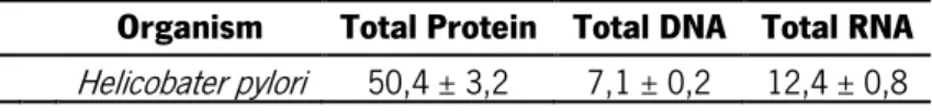
The experimental methodology to calculate the macromolecular composition of biomass (protein, DNA and RNA) was implemented in this work and the macromolecular composition was experimentally determined for Helicobacter pylori. The macromolecular composition was obtained determining the mean of 3 experimental replicas and the respective standard deviation value. The results are in Table 3.

Table 3. Experimental values of the macromolecular components Protein, DNA and RNA.

Organism Total Protein Total DNA Total RNA

Helicobater pylori 50,4 ± 3,2 7,1 ± 0,2 12,4 ± 0,8

The values obtained experimentally are significantly different from the values adopted from Escherichia coli determined by Neidhardt (Neidhardt et al, 1996) and used in the metabolic model iIT341 GSM/GPR from Helicobater pylori (Thiele et al., 2005). The differences are more substantial in DNA (129%) and RNA (40%). This result corroborates that the macromolecular composition of related organisms (in this case gram-negative organisms) can be significantly disimilar.

3.3 In silico Biomass coefficients estimation

The estimation of the amino acids, dNTPs and NTPs coefficients for the biomass equation was performed using a java tool that uses FASTA files with the sequences of interest of each organism, following the protocol published by Thiele and Palsson (Thiele et al, 2010) and described in the methods section. To estimate amino acid, dNTPs and NTPs coefficients, the macromolecular content for protein, DNA and RNA for each organism is needed. All the experimental data used in this work was found in the references in Table 2

Only bacteria were used in this study due to the lack of information for the other organisms in databases. All of the experimental and estimated coefficients for each organism are represented in the Table A 1 in annexes.

Analyzing the data from Table A 1 in annex, it can be seen that not all of the organisms have experimental data for macromolecular compositions. For C. acetobutylicum and V. vulnificus the macromolecular composition was adopted from similar organisms, B. subtilis and E. coli, respectively. In

17 general, it is assumed that the biomass composition is very similar among negative and gram-positive organisms (Neidhardt et al, 1996). For that reason, in some cases, biomass compositions from related organisms are adopted (Henry et al, 2010). However, when we analysed the macromolecular compositions that were experimentally determined, significant differences between organisms could be seen. To quantify the differences among related organisms, the difference between macromolecule compositions of each gram-negative organism and the E. coli composition (Table 4), and between gram-positive organisms and B. subtilis were calculated in percentages (Table 5).

Table 4. Differences between macromolecular composition of gram-negative organisms and E. coli.

Differences (%) _{succiniciproducens} M. _putida P. _typhimurium S. _vulnificus V. Macromolecular composition

Protein 8,00 9,09 0,09 0,00*

DNA 9,68 9,68 14,63 0,00*

RNA 2,44 2,44 9,21 0,00*

*Macromolecular composition adopted from E. coli.

Table 5. Differences between macromolecular composition of gram-positive organisms and B. subtilis.

Differences (%) _{acetobutylicum} C. _glutamicum C. _plantarum L. _lactis L. Macromolecular composition

Protein 0,00* 1,59 43,41 12,94

DNA 0,00* 61,54 26,92 11,54

RNA 0,00* 23,66 37,40 63,36

*Macromolecular composition adopted from B. subtilis.

For gram-negative organisms, the average of differences between the macromolecular composition is about 7%, but for gram-positive organisms the differences are around 30%.

Table A 1 in annex has also experimental and in silico data for amino acids, dNTPs and NTPs coefficients. Some differences can be noticed between experimental (in vivo) and in silico data. In vivo and in silico data for amino acids, dNTPs and NTPs were compared and an average, the maximum and the minimum of the percentage of differences between in vivo and in silico data were calculated, and are shown in Table 6.

18 Table 6. Average, maximum and minimum differences, between in vivo and in silico data, for amino acids, deoxynucleotides and nucleotides.

Differences

vivo/silico (%) Bsu Cac Cgl Eco Lpl Lla Msu Ppu Sty Vvu Amino Acids Average 24,0 105,1 440,2 18,1 33,0 28,4 189,5 1078,0 85,4 23,8 Maximum 70,7 390,8 3417,9 43,9 127,0 94,0 3049,4 20544,8 310,9 83,7 Minimum 0,8 12,7 2,5 0,1 3,0 0,9 1,9 7,6 0,02 0,2 Deoxyucleotides Average 4,11 0,19 0,24 0,08 0,95 0,38 0,56 0,42 0,03 0,56 Maximum 6,90 0,50 0,48 0,13 1,27 0,82 1,03 0,74 0,04 0,88 Minimum 0,36 0,02 0,02 0,03 0,72 0,02 0,23 0,03 0,01 0,30 Nucleotides Average 13,07 18,82 10,49 22,15 20,59 28,05 25,61 16,72 16,36 7,34 Maximum 30,81 31,79 16,36 34,20 61,85 43,02 42,37 21,72 28,44 13,26 Minimum 1,61 4,63 4,38 16,61 0,69 14,84 15,93 9,87 4,30 3,24

Analyzing the amino acid composition, it can be seen that the average differences are substantial. This was expected since in silico estimation presumes that all proteins are being expressed at the same time and in the same amount, a fact that is known to be false.

The amino acids with major differences to experimental data are glutamate, glutamine, cysteine and tryptophan. This fact can also be explained by some difficulties in identifying amino acids with experimental methods after protein hydrolysis. The acid hydrolysis in commonly used as the experimental method prior to amino acid determination (Fountoulakis et al, 1998) and this method converts glutamine into glutamate and the determination of the two amino acids is lumped in glutamate (Joergensen et al, 1995). The amount of glutamate is then divided in equal parts for estimating glutamate and glutamine percentages. It is thus assumed that glutamate and glutamine are in the same proportions in the protein, a fact that is known to be false.

During acid hydrolysis, tryptophan is also destroyed and cysteine cannot be detected directly from hydrolyzed samples. There are some protective reagents, such as thiaglycolic acid, phenol and 3,3-dithiodipropionic acid (DTDPA), that are added to samples before hydrolysis to protect these amino acids (Tuan et al, 1997). However, these reagents do not assure the total recovery of tryptophan and cysteine, leading to inaccurate percentage values in protein.

It was not expected that the differences for dNTPs and NTPs compositions were so significant. Even for organisms for which dNTPs and NTPs compositions were reported to be estimated from genome information, using the organism sequences in databases, there are differences. Nevertheless, major differences are seen for NTPs composition. This fact can be explained by the use of different methods to calculate the NTPs composition. Some authors estimate NTPs composition accounting only with open

19 reading frames sequences (Raghunathan et al., 2009). Other authors use genomic DNA sequences to calculate the percentage of messenger RNA (mRNA) (Kjeldsen et al., 2009 and Sohn et al., 2010b).

Small differences can also be justified by the use of different databases to retrieve the sequences of each organism and the existence of differences between these sequences. It has been also noticed that, in some cases, the percentage of dNTPs and NTPs is not calculated from all sequences of an organism but from fragments or samples of the total sequences (642 nucleotides for DNA and RNA) (Sohn et al, 2010a).

3.4 In silico Simulations

As it could be noticed in Table 4, Table 5, and Table 6, there are some differences between macromolecular and building blocks compositions between organisms and between in vivo and in silico data. In order to verify if these differences have impact in specific growth rate predictions and in flux distribution values, in silico simulations were performed using the Optflux 3.06 software tool.

3.4.1 Sensitivity analysis

In a first step, a sensitivity analysis of model predictions to the biomass coefficients was performed. For that purpose, the SBML version of the iAF1260 model of Escherichia coli (Feist et al, 2007) was used. This sensitivity analysis was performed using a developed java tool, by varying each coefficient (macromolecule or building block) with a factor of 5%, 7.5%, 10% and 50% (plus and minus). The values used have taken into account the differences previously obtained and shown in Table 4, Table 5 and Table 6. For each factor modification, a wild-type simulation was performed and the specific growth rate and the flux values of all reactions were obtained (see Table A 2 in annex and in excel file in supplementary material respectively).

To analyze the differences between the values obtained for each coefficient variation and the experimental value, the percentage of the difference of the specific growth rate was calculated, together with the average flux difference.

In Table A 2 it can be seen that, for the sensitivity factors of 5% and 7.5%, the overall impact is low. However, some differences can be observed for specific building blocks components and for higher variations. The data sensitivity analysis for the most relevant components is thus summarized in Table 7 and Table 8.

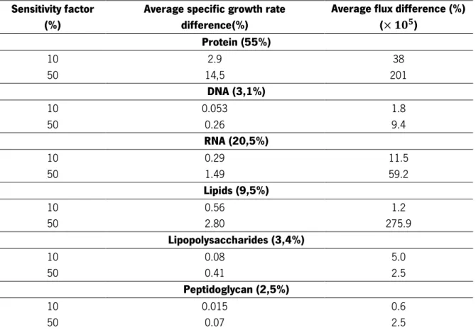
20 Table 7. Sensitivity analysis of macromolecular coefficients variation for sensitivity factors of 10% and 50%. Nominal composition is given in parentheses.

Sensitivity factor (%)

Average specific growth rate difference(%)

Average flux difference (%) ( ) Protein (55%) 10 2.9 38 50 14,5 201 DNA (3,1%) 10 0.053 1.8 50 0.26 9.4 RNA (20,5%) 10 0.29 11.5 50 1.49 59.2 Lipids (9,5%) 10 0.56 1.2 50 2.80 275.9 Lipopolysaccharides (3,4%) 10 0.08 5.0 50 0.41 2.5 Peptidoglycan (2,5%) 10 0.015 0.6 50 0.07 2.5

In Table 7 it can be seen, as expected, that the differences for macromolecular coefficients are more significant for the sensitivity factor of 50%. The differences are bigger for protein and smaller for peptidoglycan. However, this fact is due to the fact that protein is the macromolecule that has a highest percentage in biomass composition (55%) while peptidoglycan is the macromolecule that has the smallest percentage in biomass composition (2.5%). The most revealing fact in these results is that the lipid composition has a significant impact in the flux distributions, when comparing to its original percentage in total biomass composition.

21 Table 8. Sensitivity analysis of the building blocks coefficients variation (top 20) for a sensitivity factor of 50%.

Building block Differences to growth rate

Experimental value (%)

Average flux distribution differences (%) ( ) gly 0.596 20.3 leu-L 0.583 27.6 ile-L 0.564 1.33 phe-L 0.512 7.75 asp-L 0.501 8.49 asn-L 0.451 5.80 glu-L 0.397 16.5 met-L 0.387 17.9 gln-L 0.342 4.48 ala-L 0.300 8.75 ser-L 0.297 3.91 lys-L 0.296 4.27 val-L 0.279 20.3 arg-L 0.276 16.5 tyr-L 0.241 3.86 pro-L 0.171 5.97 trp-L 0.160 2.91 atp 0.124 11.7 thr-L 0.085 573 utp 0.066 11.6

In Table 8, the top 20 building blocks are represented that showed the greater impact in predicting the specific growth rate. It can be verified that 18 out of the 20 building blocks are amino acids. This can be explained by the fact that the amino acid composition in biomass is affected by the percentage of total protein and that protein is the major component in biomass. It can thus be concluded that, of all the building blocks, amino acids are the ones that have the greatest influence in specific growth rate predictions for E. coli. However, as it was noticed for the macromolecular composition, the differences for the specific growth rates do not depend only on the original percentage of each amino acid in the protein composition. For example, the amino acid phenylalanine does not have a high percentage in the total protein (3.46%) but is one of the amino acids that has a major impact in growth rate predictions (see Table A 1 for amino acid percentage in E. coli). The same conclusion can be made when analyzing

22 the average flux differences. In this case, the amino acid that originates the greatest differences in flux distribution is threonine, that has a percentage in total protein of 4.76%.

3.4.2 Impact of Biomass composition in specific growth rate predictions

In order to analyze the impact of the use of in silico, E. coli and B. subtilis biomass compositions, in silico simulations were performed using Optflux 3.06 , and the specific growth rate of each simulation was compared with the specific growth rate obtained using the experimental biomass composition included in the model. The models that were used are those in Table 1. For each model, the coefficients of the biomass equation for macromolecular composition and building blocks were altered (replaced by the compositions from E. coli, B. subtilis and in silico computed), and the specific growth rate was obtained. All the simulation results and the specific growth rates obtained are in Table A 3 in annex. To compare the specific growth rates, the percentage of the difference between each specific growth rate determined with altered biomass equations and with the experimentally determined ones were calculated. These differences are summarized in Table A 4 in annex.

The bar plots in Figure 3 represent, for each organism, the differences on the specific growth rates obtained using the in silico and the experimental coefficients (see Table A 1 in annex for further details). It should be noticed that, for these comparisons, the macromolecular composition was kept, as those values cannot be predicted in silico.

Analyzing the bar plots of Figure 3 it can be seen that for all organisms (exception made for V. vulnificus) the specific growth rates obtained using the in silico biomass compositions are very similar to the specific growth rates obtained using the experimental composition (differences of less than 1,5%). For all organisms, the specific growth rate obtained for in silico dNTPs composition is almost equal to the specific growth rate obtained using experimental values. The major differences to the experimental specific growth rate are found in nucleotide compositions. The revealing fact in these results is the big differences observed in specific growth rates for altered nucleotide compositions for V. vulnificus (near 20%). However, the coefficients used in the model (experimentally determined) are not very different from the in silico coefficients (see Table A 1 in annex for the in silico percentages for nucleotides composition of V. vulnificus). This fact can be interpreted by the hypothesis that one or more of the nucleotides have an important role in the V. vulnificus’ metabolic network.

23 Figure 3. Differences for growth rate predictions between using experimental and in silico biomass composition for each organism studied, represented in percentage. AA represents amino acids coefficients, dNTPs represents deoxynucleotides coefficients, NTPs represents nucleotides coefficients and All represents simultaneous changes in amino acids, deoxynucleotides and nucleotides coefficients.

The bar plots in Figure 4 again represent, for each organism, the differences on the specific growth rate predictions between using the experimental values and the in silico coefficients, and also using macromolecular coefficients coming from E. coli and B. subtilis (see Table A 4 in annex).

AA dNTPs NTPs ALL 0 5 10 15 20 Bacillus subtilis AA dNTPs NTPs ALL 0 10 20 Lactobacillus plantarum AA dNTPs NTPs ALL 0 5 10 15 20 D if fe re n c e s t o E x p e ri m e n ta l D a ta ( % ) Lactococcus lactis AA dNTPs NTPs ALL 0 5 10 15 20 D if fe re n c e s t o E x p e ri m e n ta l D a ta ( % ) Pseudomonas putida AA dNTPs NTPs ALL 0 5 10 15 20 Biomass Composition Salmonella typhimurium AA dNTPs NTPs ALL 0 5 10 15 20 Biomass Composition Vibrio vulnificus

24 Figure 4. Differences for the specific growth rates predictions between experimentally determined biomass composition and three other setups: using in silico building blocks composition together with experimental macromolecular composition for the studied organism (IS), original (experimental)building blocks composition and E. coli macromolecular composition (E. coli) and original (Experimental)building blocks composition and B. subtilis macromolecular composition (B. subtlis).

Analyzing the bar plot of Figure 4 it can be seen that, for all organisms (exception made for V. vulnificus) the specific growth rates obtained using the in silico compositions are very close to the specific growth rate obtained using the experimental composition. These values are closer than when other macromolecular compositions are used (even keeping experimentally determined building blocks composition), again indicating that, with the exception of V. vulnificus, in silico building block composition could be used if the macromolecular composition is known. In the case of V. vulnificus, the differences to the results obtained using E. coli macromolecular composition is null because the macromolecular composition of V. vulnificus was adopted from E. coli. For gram-positive organisms, when the macromolecular composition of single macromolecules (protein or DNA or RNA) is replaced by B. subtilis’ composition, the differences obtained are smaller than when the data comes from E. coli (data shown in

IS E. coli B. subtilis 0 20 40 60 Bacillus subtilis IS E. coli B. subtilis 0 20 40 60 Lactobacillus plantarum IS E. coli B. subtilis 0 20 40 60 D if fe re n c e s t o E x p e ri m e n ta l D a ta ( % ) Lactococcus lactis IS E. coli B. subtilis 0 20 40 60 D if fe re n c e s t o E x p e ri m e n ta l D a ta ( % ) Pseudomonas putida IS E. coli B. subtilis 0 20 40 60 Biomass Composition Salmonella typhimurium IS E. coli B. subtilis 0 20 40 60 Biomass Composition Vibrio vulnificus

25 Table A 4 in annex). However, the same trend in not always valid when all the macromolecules are changed, as it can be seen in Figure 4.

For gram-negative organisms, as expected, when the macromolecular compositions of single macromolecules (protein or DNA or RNA) or when all the macromolecular composition is replaced by E. coli composition, the differences on the specific growth rate are smaller than the differences obtained when B. subtilis data are used.

The bar plots in Figure 5 represent, for each organism, the differences on the specific growth rate between original predictions and three setups: the use of in silico building block coefficients (with original macromolecular compositions), macromolecular and building blocks coefficients from E. coli, and from B. subtilis (see Table A 4 in annex).

Figure 5. Differences for the specific growth rates predictions between experimentally determined biomass composition and three other setups: using in silico building blocks composition together with experimental macromolecular composition for the studied organism (IS), building blocks and macromolecular composition from E. coli (E. coli) and building blocks and macromolecular composition from B. subtilis (B. subtlis)

In the bar plots in Figure 5 it can be seen that in all of the cases (exception made for V. vulnificus) the smallest difference to the experimental data is obtained with the coefficients estimated from

IS E. coli B. subtilis 0 50 100 Bacillus subtilis IS E. coli B. subtilis 0 50 100 Lactobacillus plantarum IS E. coli B. subtilis 0 50 100 D if fe re n c e s t o E x p e ri m e n ta l D a ta ( % ) Lactococcus lactis IS E. coli B. subtilis 0 50 100 D if fe re n c e s t o E x p e ri m e n ta l D a ta ( % ) Pseudomonas putida IS E. coli B. subtilis 0 50 100 Biomass Composition Salmonella typhimurium IS E. coli B. subtilis 0 50 100 Biomass Composition Vibrio vulnificus