Universidade do Minho
Escola de Engenharia
Pedro Emanuel Pereira Soares
Computer vision component to environment
scanning
Universidade do Minho
Escola de Engenharia
Pedro Emanuel Pereira Soares
Computer vision component to environment
scanning
Dissertação de Mestrado
Área de Especialização Informática
Trabalho efectuado sob a orientação do
Professor Doutor Manuel João Ferreira
Computer vision component to environment
scanning
Pedro Emanuel Pereira Soares
Computer vision is usually used as the perception channel of robotic platforms. These platforms must be able of visually scanning the environment to detect specific targets and obstacles. Part of detecting obstacles is knowing their relative distance to robot. In this work different ways of detecting the distance of an object are analyzed and implemented. Extracting this depth perception from a scene involves three different steps: finding features in an image, finding those same features in another image and calculate the features’ distance. For capturing the images two approaches were considered: single cameras, where we capture an image, move the camera and capture another, or stereo cameras, where images are taken from both cameras at the same time. Starting by SUSAN, then SIFT and SURF, these three feature extraction algorithms will be presented as well as their matching procedure. An important part of computer vision systems is the camera. For that reason, the procedure of calibrating a camera will be explained. Epipolar geometry and the fundamental matrix are two important concepts regarding 3D reconstruction which will also be analyzed and explained. In the final part of the work all concepts and ideas were implemented and, for each approach, tests were made and results analyzed. For controlled environments the relative distance of the objects is correctly extracted but with more complex environment such results are harder to obtain.
Keywords: Computer Vision; 3D reconstruction;
Resumo
A visão por computador é, normalmente, usada como o canal de percepção do mundo em plataformas robóticas. Estas plataformas têm de ser capazes de rastrear, visualmente, o ambiente para detectar objectivos e obstáculos específicos. Parte da detecção de obstáculos envolve saber da sua distância relativa ao robot. Neste trabalho, são analisadas e implemen-tadas diferentes formas de extrair a distância de um objecto.
A extracção desta noção de profundidade de uma cena envolve três passos diferentes: encontrar características numa imagem, encontrar estas mesmas características numa im-agem diferente e calcular as suas distâncias. Para a captura de imagens foram considerados dois métodos: uma única câmara, onde é tirada uma imagem, a câmara é movida e é tirada a segunda imagem; e câmaras estéreo onde as imagens são tiradas de ambas as câmaras ao mesmo tempo. Começando pelo SUSAN, depois o SIFT e SURF, estes três algoritmos de ex-tracção de características são apresentados, assim como os seus métodos de emparelhamento de características.
Uma parte importante dos sistemas de visão por computador é a câmara, por este motivo, o procedimento de calibrar uma câmara é explicado. Geometria Epipolar e matriz funda-mental são dois conceitos importantes no que refere a reconstrução 3D que também serão analisados e explicados. Na parte final do trabalho, todos os conceitos e ideias são imple-mentados e, para cada método, são realizados testes e os seus resultados são analisados. Para ambientes controlados, a distância relativa é correctamente extraída mas, para ambientes mais complexos, os mesmos resultados são obtidos com mais dificuldade.
Palavras chave : Visão por computador; reconstrução 3D;
1 Introduction 1
1.1 Motivation. . . 1
1.2 Objectives . . . 2
1.3 Structure of Report . . . 2
2 Image Processing - point extraction 3 2.1 Introduction . . . 3
2.2 SIFT-features Algorithm . . . 4
2.2.1 Steps . . . 5
2.3 SURF-features Algorithm . . . 7
2.3.1 Interest point detection . . . 7
2.3.2 Interest point description and matching . . . 10
2.4 SUSAN Algorithm with Kirsch . . . 13
2.4.1 SUSAN Corners . . . 13
2.4.2 Kirsch Edge Detector . . . 16
2.4.3 All together . . . 17 3 3D Reconstruction 18 3.1 Introduction . . . 18 3.2 Camera calibration . . . 18 3.2.1 Camera Matrix . . . 19 3.2.2 Methods . . . 22 3.2.3 Stereo Cameras . . . 26 3.3 Reconstruction . . . 29 3.3.1 Epipolar Geometry . . . 29 3.3.2 Fundamental matrix . . . 30 3.3.3 Reconstruction . . . 32 4 Development process 35 4.1 Introduction . . . 35 iii
4.2 Common work . . . 36 4.3 Point extraction . . . 37 4.3.1 SIFT Algorithm . . . 38 4.3.2 SURF Algorithm . . . 41 4.3.3 SUSAN Algorithm . . . 45 4.4 3D Reconstruction . . . 48
4.4.1 Single Camera Approach . . . 49
4.4.2 Stereo Cameras Approach . . . 55
5 Conclusion 62
Bibliography
2.1 Same object from two different perspectives . . . 4
2.2 Integral Image sum of intensitiesP= I(A) + I(D) − I(B) − I(C) . . . . 8 2.3 Non-maxima Suppression. . . 10
2.4 Haar Wavelets. . . 11
2.5 Wavelets Sum. In this case the assigned orientation would be the one in last image. . . 11
2.6 USAN area . . . 13
2.7 Corner USAN area . . . 16
3.1 Pinhole geometry. Note that the image plane is in front of the camera . . . . 19
3.2 Planar Homography . . . 23
3.3 Stereo Calibration . . . 27
3.4 Stereo Rectification . . . 28
3.5 Rectified Image . . . 29
3.6 Epipolar geometry . . . 30
4.1 Simulated robots in Webots.The grey blocks represent the cameras . . . 36
4.2 Test images . . . 38
4.3 SIFT Image Results . . . 40
4.4 SURF Image Results . . . 44
4.5 SUSAN Image Results . . . 48
4.6 Webots images . . . 52
4.7 3D results from Webots images . . . 53
4.8 Real images . . . 53
4.9 3D results from Real images . . . 53
4.10 Stereo camera images . . . 54
4.11 3D results from Stereo cameras images . . . 54
4.12 SUSAN Image Results with better matching algorithm . . . 58
4.13 Control environment SIFT SURF and SUSAN . . . 59
4.14 Stereo reconstruction with Webots images . . . 60 v
4.15 Stereo reconstruction with real images . . . 60
4.16 Distance plotting in moving object. . . 60
4.17 Distance in detected objects. . . 61
4.1 SIFT results . . . 39
4.2 SURF results . . . 44
4.3 SUSAN results . . . 47
Chapter 1
Introduction
We can say that vision is a very, if not the most, important sense when we are moving in a certain environment. Providing crucial information about the environment, one relies, must of the times, only on vision to guide ourselves in a world full of obstacles. The importance of vision in animals and humans can also be seen in robots. In various robotic platforms, the vision system is the main perception device and robots must be able to rely on it to move and detect objects in the world.
When an image is captured by computer vision systems a lot of information is obtained but despite all that information, the depth of a scene point is not directly accessible. It is easily understood that knowing the 3D localization of an object in space is very important when talking about a moving robot. If there is no 3D information the robot that, for example, finds an obstacle in its path does not know if the obstacle is near and it needs to be avoided or if it is far away and there is no need to avoid it at the moment.
In this work we will discuss and implement different approaches to the problem of ex-tracting 3D information from a scene. Different approaches to the image processing step will be analyzed and the results compared. When extracting 3D information we will test two different approaches, single and dual camera system.
1.1
Motivation
Focusing merely on vision, the capability that the brain has of extracting information from what our eyes see is simply amazing. There are computer vision systems that are faster and have better performance in certain tasks, but generally, we are still faster and better. One area where the human brain exceeds computer vision is the detection of objects and 3D information extraction. By looking at a room we know, for example, which objects are closer to us and when walking, if see an object, in this case an obstacle in our way, we know if have to move around it or if it is still far away. Regarding moving robots, this vision capability
would be a very good thing to have.
In computer vision when an image is obtained from a camera we only have 2D informa-tion, that is, x and y position. With this information we can say that a certain point is more to the left/right or higher/lower but we cannot say if it is closer or further from us. Correctly extracting the third coordinate z, allowing us to extract 3D information from a scene, is the objective of this work. Having correct 3D information from a scene will give the robot better moving abilities.
1.2
Objectives
In order to complete our main objective of extracting 3D information from a scene, three steps must be accomplished.
• Point Extraction - Given images we should be able to extract defining points.
• Point Comparison - We must be able to find the same points in two different images. • 3D Reconstruction - From the information received from previous steps we have to
extract 3D information.
1.3
Structure of Report
In Chapter 2 we will talk about the first step of the 3D reconstruction, image processing. In this chapter we will analyze different approaches to the problem of extracting and comparing points in an image. The process of 3D reconstruction will be explained in chapter 3. Starting by explaining why and how to calibrate a camera following on what is the fundamental matrix and what is it used for, and, finally the triangulation. After explaining the ideas and methods used, we will show how this methods were implemented and tested and the results obtained in each method in chapter 4. We will finish this work with a conclusion, explaining the results obtained and the problems encountered.
Chapter 2
Image Processing - point extraction
2.1
Introduction
As mentioned before an image can only give us 2D information. When we look at a photo, for example, we can tell which objects are closer or further away, but, this perception is not only based in the information of the photo, one needs extra information to accurately perceive the distances. One of that extra information is the common size of the object or, by other words, what we think that the size should be. Let us consider the following situation: an oversized beer can and a small car model, in a proportion that gives them similar sizes. If we place the can and the car next to each other and take a photo what will we see? We will see a can and a car with the same size and the brain will assume that the can is closer to the camera (since we know that a can should be smaller than a car).
So, how can we extract 3D information from images (without knowing the size of ob-jects)? We need at least two images of the same scene from different perspectives. This can be done in two ways: with two cameras (stereo correspondence) or with one moving camera (structure from motion). Usually the more cameras being used the better: this project will use two cameras. Even humans need two images to extract 3D information. If we close one eye, after a while, we will lose the 3D perspective, unless we move therefore obtaining images from different perspectives.
The basic idea of 3D extraction from images is matching them and computing the differ-ences. Image matching is a very important step in many computer vision problems such as solving 3D structure from multiple images an stereo correspondence. Matching two images is usually done by finding distinctive points (features) in one and finding the same points in the other. When talking about image matching for 3D reconstruction, especially in moving environments, it must be taken into account that the camera will move and lighting condi-tions will probably change as well. For that, the image matching algorithm must be prepared to find and match features even in those conditions. In image matching finding the features is
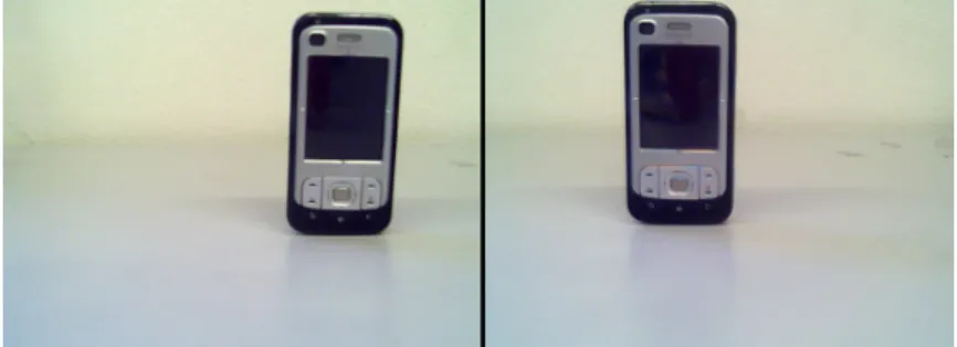
Figure 2.1: Same object from two different perspectives
not a simple procedure. One can have lots of features but if finding them again in the second image is impossible, we will not be able to match both images. An algorithm must provide us a way of differentiating a feature from another (i.e. a descriptor) so we can know if the point we find is the same that we found before.
When classifying an feature detection algorithm for image matching there are some cri-teria for determining its quality:
• Quality of detection
When finding features in an image the algorithm should produce very few false posi-tives, usually originated from noise.
• Consistence
If an image is tested several times the same feature points should be detected. • Speed of detection
As for most types of algorithms, the time it takes to produce results should be mini-mum.
• Quality of descriptor
As mentioned before, what use do we have for lots of points if we can’t correctly find and match them in another image.
• Speed of matching
In image matching algorithms a relatively big portion of time is spent in comparing and matching points.
2.2
SIFT-features Algorithm
Scale-invariant feature transform (SIFT) algorithm proposed by Lowe in [22, 23] is a com-monly used algorithm used in computer vision to detect local features in images.
2.2. SIFT-FEATURES ALGORITHM 5
Scale-invariant feature transform, as the name suggests, focus on features that are in-variant to scaling and rotation and also partially inin-variant to change in illumination and 3D camera viewpoint. SIFT algorithm also performs rather well when occlusion, clutter, or noise occur in an image.
Fortunately, SFIT found features are also very distinctive making them relatively easy to match in other images. Large numbers of distinctive features can be efficiently extracted from images and then matched with SIFT making it very useful in image matching. In the next section we will present the normal use of the SIFT algorithm.
2.2.1
Steps
In order to generate a set of distinctive scale-invariant image features several steps must be taken. We can organize the process in four major steps. In early steps of the process several points are found and if we were to apply the most expensive operations of the algorithm to all points the algorithm’s efficiency would be compromised. So in order to increase efficiency, initial tests are made to the points to determine which ones are worth passing to the next stage. By doing so we guarantee that the most expensive operations are applied only to those points that pass initial tests minimizing the cost of the algorithm.
Interest point localization
The first stage of the SIFT’s algorithm is finding scale invariant points, called interest points, so they can be examined in further detail in the next steps. This is done by searching over all scales and image locations and selecting those locations that are stable across all scales. A
difference-of-Gaussianis applied to obtain different scales.
L(x, y, σ)= G(x, y, σ) ∗ I(x, y) (2.1)
Function 2.1 defines a scaled image L(x, y, σ) obtained from applying to an image I(x, y) a scale variable G(x, y, σ). When 2.1 is applied to an input image I we get a different scaled image L.
D(x, y, σ)= L(x, y, kσ) − L(x, y, σ) (2.2)
Function 2.2 defines de difference-of-Gaussian (DoG) between two images where one has a k times bigger scale. After the DoG is applied each point of the image is compared with both neighbors at different scales. Considering a point in a scale k there are 8 neighbors
in the same scale and 9 in the k − 1 and k+ 1 scales making a total of 26 neighbors. If the
Key point localization
In the first, step several interest points were found but, to increase efficiency, the number of points must be reduced. This is done by selecting key points based on their stability. Scale and location is determined to each point and those points that have a low contrast (therefore sensitive to noise) are rejected. First for each interest point, its position is determined by interpolation of nearby data, this is done using the quadratic Taylor expansion of the DoG which gives an offset. If the offset is larger than 0.5 the point is close to another interest point so we will change to that point and an interpolation is performed. If the offset is equal or less than 0.5 it will be added to the interest point being analyzed giving an approximated localization. Using the Taylor expansion again, if the offset is less than 0.03 the interest point is discarded for having a very low contrast. Low contrast points are very sensitive to light alterations and therefore, very unstable. Because DoG function is very sensitive to edges, resulting in a lot of interest points in edge lines, points that have poorly determined location but high edge response must be eliminated. After this step all points are now considered key points.
Orientation assignment
This is the step where rotation invariance will be achieved. To each key point one or more orientations will be assigned based on local image gradient directions. The invariance to rotation is achieved because all future operations will be performed relative to the assigned orientation. To find the correct orientation, an histogram of gradient orientations is created based on the point’s neighbor. The peak orientation of the histogram is assigned to the point.
Key point descriptor
From the previous steps the algorithm was able to achieve scale, rotation and location in-variance. This step aims to achieve illumination and 3D viewpoint invariable. This is done by assigning a highly distinctive descriptor to each key-point. The key point descriptor is created from magnitude and orientation gradients of the area around the key point. This step is performed on the closest scale image.
Key point matching
As we told before, for image matching we need more than scale-invariant features found in an image. If we cannot match the features found in an image to those found in another image, matching is not possible. SIFT gives a highly distinctive descriptor for each key point, making it a reliable method even when large features databases are being used. Normally when features are extracted they are stored in various ways and when a new image is captured
2.3. SURF-FEATURES ALGORITHM 7
and its features extracted, each of the new points must be compared to stored points for a match. [23] shows a good reliability even when large databases are used. Two important determinants of SIFT’s algorithm performance are: how the points are stored and how the search is made. Searches in large databases can sometimes be a bottleneck to algorithms performance. KD-Tree [14] is a normally used data structure that allows for points to be organized in space according to the value. This kind of data structure is used in applications where we have to find the values closest to a given value. As in any tree-organized data structure any search for a given value is much more efficient than regular searches.
2.3
SURF-features Algorithm
Speeded Up Robust Feature (SURF) [1] [2] is another feature extraction and matching algo-rithm also intended to be scale and rotation invariant. Although it is based on SIFT, it is said be faster and have better performance against image transformations. One of the reasons of it’s speed is the use of Integral Images as an aid structure throughout the rest of the process. It is also based in Hessian detectors, as it was done by Lindberg [20], for the extraction of in-terest points, and Haar Wavelet [10] responses as the points descriptors. As for SIFT, SURF as two important stages: interest point detection and point descriptor matching.
2.3.1
Interest point detection
As in many other algorithms, we must start by finding interest points.In SURF this is done in four sub-steps starting by using Integral Images as a helpful way to speed things up. Using a Hessian detector we then find interest points across the image and construct a scale space representation. The final step in interest point detection is to use non-maximum suppression.
Integral Images
Integral Images or Summed Area Table first appeared in [6] and have become very useful in box type convolution filters. When for each pixel we compute something based on a mask, such as circular mask in SUSAN, we have a convolution filter. In order to use integral images, the filter mask must have a box shape because Integral Images use rectangles as the base of calculation. I(x, y)= i0<x X i=0 j≤y X j=0 I(i, j) (2.3)
From 2.3 we can see that for each pixel A= (x, y) it’s integral image result will be the sum
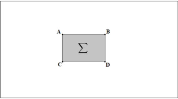
all pixels within a rectangle defined by (0, 0) and (x, y). The reason why Integral Images are so useful is that for any pixel, we can find the sum of intensities of the surrounding area with just three operations and four memory accesses, as showed in figure 2.2. The time in which we can find a result in an Integral image is independent of filter size, this is very important as SURF usually uses big filters
Figure 2.2: Integral Image sum of intensitiesP = I(A) + I(D) − I(B) − I(C)
Moreover Integral Images are relatively easy to compute as we only need one pass over the image.
I(x, y)= i(x, y) + I(x − 1, y) + I(x, y − 1) − I(x − 1, y − 1) (2.4)
The fact that Integral Images are fast to compute and make finding the sum of intensities an easy and fast task, is one of the reasons for SURF speed.
Hessian Detector
The previous step was only to give us a way to speed calculations involving sums of inten-sities. Now we will start the process of finding those points using an Hessian-based detector for every pixel.
H(X, σ)= Lxx(X, σ) Lxy(X, σ) Lxy(X, σ) Lyy(X, σ) (2.5)
In equation 2.5 H(X, σ) defines the Hessian matrix at point X where Lab(X, σ) is the
Gaussian second derivative in the a and b directions. These derivatives are computed for the smoothing scale σ, which has the same meaning as in equation 2.1 in Section 2.2.1. Box filters are used to approximate the results of these second order Gaussian derivatives and can
be evaluated using integral images at low cost. For a real valued Gaussian with σ = 1.2 the
box filter that approximates result will have a size of 9 ∗ 9.
In a Hessian matrix the value of its determinant is used to classify the maxima and min-ima by the second derivative test. In SURF the determinant’s sign is used to classify the point.
2.3. SURF-FEATURES ALGORITHM 9
det(H)= LxxLyy− (wLxy)2 (2.6)
For each pixel we can calculate the determinant and use it to classify the point. We can consider a point as an extremum if its discriminant is positive. We refer to this determinant as the blob response and all responses are stored in a blob response map over different scales. They will later be used to locate interest points.
Scale Space representation
In order for the algorithm to be able to detect the same point over different scaled images, we need to search for interest points across the different image scales. We therefore need a structure that allows us to represent this scale space. In computer vision pyramids are used to implement this scale space. Starting, with the original image at the base level of the pyramid we smooth, using Gaussian, and sub-sample (reduced in size) it to get to the next level of the pyramid. This method of creating an image pyramid is used in SIFT but, with the help of integral images and box filters, this computationally heavy step is improved in SURF. The use of integral images and box filters allows SURF to apply box filters of any size directly on the same image with a constant speed, instead of reapplying the same filter to a previously filtered image. This is a considerably big difference between image pyramids used in SIFT since we upscale the filter size rather than reduce the image size. As mentioned before "normal" image pyramids are computationally heavy, on the other hand, SURF image pyramids are not. This is another reason why the SURF algorithm is faster.
In SURF, this image pyramid is divided into octaves and each octave refers to a series of response maps. These octaves are then subdivided into a constant number of scale levels. For the first level of the pyramid, a 9 ∗ 9 sized filter is used and for subsequent layers the filter is up-scaled. At any iteration the next scale the window has to increase a minimum of 2 pixels, since we always need a center pixel.
Points Location
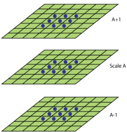
Now that we have the image pyramids constructed for each pixel, we have to find those that are invariant to scale and rotation and therefore points of interest. First we start by using a threshold to eliminate all points that have responses below the predetermined threshold. With this we can control the quantity of points detected and we can choose to increase the threshold and, by this, allowing only the most invariant points to continue. Once all the points are threshold, a non-maximum suppression, as explained in section 2.4.1, is done to find the candidate points. Considering that an image is on a layer of the pyramid and there are two more layers next to it (each one of the scales above and below), we can say that a
pixel has a total of 26 neighbors as illustrated in figure 2.3.
Figure 2.3: Non-maxima Suppression.
Considering point X in figure 2.3, during non-maxima suppression, the point will be considered a maxima if it is greater than his neighbors, represented as blue balls.
After this two steps we have a set of points that are both higher than the threshold and local maxima. From here we interpolate the points using the method purpose by Brown and Lowe in [5] resulting in a set of detected features.
2.3.2
Interest point description and matching
Now that we have a set of points found in an image, we need to find the same points in a different image. Since the same method of finding points will be used in both images, chances are that points found in the first image, will be found again in the second. But there is still the question of knowing if it is the same point or not. As mentioned before we have to find a way of describing the points (i.e. a descriptor). This descriptor describes the content of the area around the pixel in terms of intensity.
Orientation assignment
As said before an image feature should be invariant to image rotation. In SURF, as in SIFT, this is done by identifying an orientation for each interest point. Like explained in section 2.2.1 all future operations will be performed relative to the assigned orientation, therefore achieving orientation invariance. Instead of gradient histograms, as used in SIFT, SURF uses Haar wavelet to find the assigned orientation. One of the uses for the Haar Wavelet is to find gradients, both in x and y directions.
To facilitate the explanation of how an orientation is found, we will divide the process into three steps. For each point we:
2.3. SURF-FEATURES ALGORITHM 11
Figure 2.4: Haar Wavelets.
• Calculate wavelets
To do this, we start by choosing a circular area around the point. This area has the radius size of 6σ, where σ is the scale in which the point was detected. For all points inside the area we calculate the wavelet responses. The wavelets used have a size of 4σ. Once again the integral images came in handy as we only need six operations to compute the response in x or y direction at any scale.
• Map responses
All wavelet responses are weighted with a Gaussian centered in the interest point. Again the scale, in which the point was detected, is taken into account and a deviation of 2.5σ is used. With all responses weighted we map them in a 2D space.
• Sum wavelets
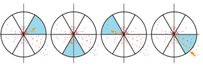
Imagining a circle in the 2D space centered at the origin, we divide this circle in 6 slices. For each slice we sum all responses within, resulting in a response vector. After all 6 vectors are calculated, the longest one is chosen as the interest point orientation.
The size of the slice, in this case Π3 can be altered although caution must be taken.
This process is exemplified in figure 2.5.
Figure 2.5: Wavelets Sum. In this case the assigned orientation would be the one in last image.
Haar wavelets based Descriptors
The process of calculating a descriptor for each point starts by constructing a square region centered in the point along the point’s orientation. This square has a size of 20σ and contains the all pixels which will take part in the calculation of the descriptor vector. The square is then divided into 16 (4 ∗ 4) sub-regions and for each one, we calculate the Haar wavelets (size 2σ), responses obtaining this way a descriptor vector.
Descriptorsubregion = [
X
dx,Xdy,X|dx|,X|dy|] (2.7)
From equation 2.7 we can see that each sub-region will have a sized 4 vector containing
dx dy which are the wavelet responses in x and y respectively and they’re absolute values
|dx||dy|. Note that these directions are defined in relation to the point’s assigned orientation. Therefore we have 4 descriptor values for each sub-region with a total of 16 sub-regions making a total of 64 values. These 64 values are the entries of the point’s descriptor vector. Another version of SURF called SURF-128 doubles the number of descriptors values. It does this by splitting the sum according to their sign, we therefore get two descriptors for each of older ones as we can see in 2.8.
Descriptorsubregion= [P dx < 0, P dy < 0, P |dx < 0|,
P |dy < 0|, P dx ≥ 0, P dy ≥ 0, P |dx ≥ 0|, P |dy ≥ 0|] (2.8)
If we double the descriptor values with the same 16 sub-regions we get 8 × 16 = 128
values. Having a descriptor with twice the number of the values, we get a more distinctive descriptor. This reduces the number of mismatches but, on the down side, even though the computing time is not much slower than normal, the matching stage is much slower.
Indexing for matching
In order to help in the process of indexing and matching, SURF uses the sign of the trace of the Hessian matrix, computed in the detection phase, as a way to differentiate points. The sign of the Laplacian (trace of the Hessian matrix) allows us to distinguish between bright blobs on dark backgrounds and the reverse. This simple and "free"(already computed) infor-mation gives a way of differentiating the points on a high level, if the points have different signs they are not a match. It is easily understood the advantages this gives us, at the index-ing phase we can create 2 areas and when searchindex-ing for a match we only have in one of the areas. Even in more complex indexing systems such as K-d trees we can split the search area therefore improving the matching time.
2.4. SUSAN ALGORITHM WITH KIRSCH 13
2.4
SUSAN Algorithm with Kirsch
In this section we will explain the methods used to attempt the extraction and matching of points. This method starts by finding points using SUSAN’s corners and giving each point a descriptor based on Kirsch Gradient.
2.4.1
SUSAN Corners
Smallest Univalue Segment Assimilating Nucleus (SUSAN),proposed by Stephen M. Smith. [26], is a commonly used algorithm in computer vision to extract features from an image. SUSAN, as many other algorithms, follows the method of applying to each pixel’s neigh-boring area a set of rules and getting a response that defines the pixel. This area, in this case, is a circular window and all pixels inside that area are compared in terms of brightness to the nucleus (center of window). This area of similar pixels is called "Univalue Segment Assimilating Nucleus" (USAN) and is later used to determine if the pixel is a corner. Im-age matching requires that a number of features are extracted from an imIm-age. When using SUSAN corners as the extractor of features, we assume that corners are the most important points. When we say that a point is the most important it means that it is an easily detectable point in a sequence of images or images from different perspectives.
The principle
The basic concept of SUSAN is having, for each pixel, a local area of similar brightness, the USAN. The USAN contains important information about the area surrounding the pixel. Considering the area of the mask window and the area of the USAN we can see in figure 2.6 why we can say that if a pixel is in a corner or edge the area of the USAN it will always be less than half the size of the window.
Figure 2.6: USAN area
In 2.6b we can see that when the nucleus is in a flat area (no corners or edges) the USAN area is at a maximum. If the nucleus lies in an edge the area will be half 2.6c and the sharper the corner the less the area of the USAN will be2.6a. The area of the USAN will decrease
as an edge is approached reaching a minimum at the correct location of the edge. Looking at the relation between the area of the USAN and where the pixel is, we can say that corners will be the minimum responses to the algorithm.
How it works
Now that we understand the principle behind SUSAN algorithm we will describe the work flow of extracting corners from an image. This process can be divided in five steps.
• Place a circular mask in each pixel.
For each pixel we start by centering a circular mask window, in most cases with a size of 37 pixels, and we compare the nucleus brightness with all the pixels inside the mask. Originally the following equation 2.9 was used to determine if a pixel had an acceptable brightness, meaning, if it’s brightness was similar to the nucleus.
c(→−r, −→r0)= 1 i f |I(→−r) − I(→−r0)| ≤ t 0 i f |I(→−r) − I(→−r0)| ≥ t (2.9)
I(→−r) and I(→−r0) are the brightness’s of any pixel and the nucleus respectively, c is the
output comparison and t is the brightness difference threshold. With t we can control the acceptable differences in brightness within the USAN. If we increase t, there-fore allowing greater differences in brightness, the algorithm will consequently give a greater number of responses. We can say, then, that t allows to control the number of responses. In 2.10 we can see later version of 2.9.
c(→−r, −→r0)= e−(I(c( − → r))−I(c(−r0))→ t ) 6 (2.10) With 2.10 we get more stable and sensitive results. While 2.9 gives us binary results, 1 or 0 depending on the threshold, with 2.10 we get continuous results between 0 and 1. Because of this, with 2.10, small variations to a pixel’s brightness will not have major effects on c.
• Define the USAN.
Now that we have a way of defining which pixels belong to the USAN, we have to calculate the number of pixels that belong to the USAN. For that we use:
n(→−r0)=X
− →r
c(→−r, −→r0) (2.11)
2.4. SUSAN ALGORITHM WITH KIRSCH 15
• Geometric threshold.
As mentioned before, we can define a pixel has being in a corner based on the relation between the area of the window and the size of the USAN. The corner response, which defines "the level of corner" that a pixel is in, can be defined as:
R(→−r0)= g − n(→−r0) i f n(→−r0) < g 0 otherwise (2.12)
R(→−r0) being the initial corner response, is determined by comparing the area of the
USAN, n(→−r0), with a geometrical threshold g. We now have two different thresholds,
gand t, while t mostly affects the quantity of responses, g also affects the quantity but
most importantly it also affects the quality of the corners. We can define the quality of a corner as it’s level of sharpness, for lower values in g only sharper corners will be detected. From figure 2.6 we can define certain values for g to get different results.
Let us consider nmaxthe maximum value that n could take, this happens when we are
looking at a flat colored area and n will have the same size as the mask window. If we
consider g = nmaxin 2.10 all points would have positive results, for g = 3nmax/4 only
pixels that are on edges or corners. Since an USAN size includes the nucleus, an edge
will always have n > nmax/2 therefore we can say that for corners, g can be defined
has nmax/2.
• Eliminate false positives.
Before we can declare a point as a corner we have to take into account that false positives will be produce. In images extracted from the real world, this can occur where the boundary limits of the image are blurred. In order to eliminate this problem a simple method was implemented and applied the points found in the previous step. If we find the center of gravity of the USAN and then the distance from it to the nucleus, we can reject those which have the center of gravity near the nucleus. A USAN from a corner will not have it’s center of gravity near the nucleus. Another problem in real images is the noise. To overcome this problem SUSAN implements a contiguity rule which states that all pixel’s, within the mask, in the direction of the center of gravity starting in the nucleus must be part of the USAN. By doing so we ensure that a corner must be part of a bigger part of the image thus eliminating single pixel’s usually created from noise.
• Find corners.
The final step on SUSAN corners algorithm is to find the correct location of the cor-ners. At this step of the algorithm, we have several points in the image which are possible corners. A corner will not have only one response in it’s area, it will have
all the points which were validated in equation 2.12. But which one of these points is
the correct point? As we can see in equation 2.10 the response is 0 if n(→−r0) ≥ g and
g − n(→−r0) otherwise, which means that the smaller the USAN area is, the bigger the
response will be. It is easily understood from figure 2.7 that the closer the nucleus is to the tip of the corner the smaller its USAN area will be and therefore the bigger the response.
Figure 2.7: Corner USAN area
Because of this, we can state that the corner will be a local maximum in the image. Therefore, to find corners we have to find local maximums in the response image. To do so SUSAN uses a non-maximum suppression. Non-maximum suppression is an algorithm that suppresses all image information that is not part of local maxima, this is done using the gradient direction and will result in a set of corner points.
2.4.2
Kirsch Edge Detector
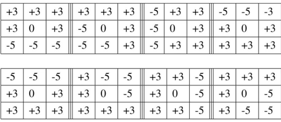
The Kirsch algorithm [18] is used to detect edges in an image using eight compass filters. Each filter is the gradient of the neighboring area of the pixel in a determined direction. For each direction, 8 in total, we apply the filter to the image and the one which has the highest response is considered as the pixel’s orientation. We then can use this maximum response to create a final image that will represent the edges of the contours.
The algorithm uses 3*3 windows for each pixel one for each direction:
+3 +3 +3 +3 +3 +3 -5 +3 +3 -5 -5 -3 +3 0 +3 -5 0 +3 -5 0 +3 +3 0 +3 -5 -5 -5 -5 -5 +3 -5 +3 +3 +3 +3 +3 -5 -5 -5 +3 -5 -5 +3 +3 -5 +3 +3 +3 +3 0 +3 +3 0 -5 +3 0 -5 +3 0 -5 +3 +3 +3 +3 +3 +3 +3 +3 -5 +3 -5 -5
2.4. SUSAN ALGORITHM WITH KIRSCH 17
When allying these filters to an image, if the pixel has a strong response it means that the pixel is in an edge. Considering grayscale images, we can say that a pixel belongs to an edge if there is another pixel next to it that has a very different level of color. If we apply the gradient to an area with the same color, not an edge, the window response will always be 0, since the sum of multipliers in the window is also 0 (ex: for the first window
3+ 3 + 3 + 3 + 0 + 3 − 5 − 5 − 5 = 0) and 0 ∗ X = 0. In the other hand, if we consider an edge
where there is an area where the pixel’s color is very different, the window response will be as high as that difference in color. Apart from giving the edges, Kirsch algorithm can also be used as a descriptor for a pixel. We can say that the descriptor for the pixel is an list of the 8 responses to the filters. When comparing the same world point in two different images chances are that pixel will have the same response to the filters.
2.4.3
All together
As mentioned before, in order to extract 3D information from a scene the first step is image matching, and for that we need points in both images and a way to match them. With SUSAN corners providing us with points we can use the Kirsch gradient as a way to give each point a descriptor to compare and match them. When find a match for the point we have to search all the other image points for the one that has a list of Kirsch values closer to the point.
3D Reconstruction
3.1
Introduction
In this work, when referring to 3D reconstruction, we mean the process of extracting 3D information from scene and interpreting it. We do not really reconstruct a scene based on images since that is not the objective of the work. The objective is to know where, relatively to us, the object is. As mentioned before the depth of a scene point is not directly accessible in 2D images. With at least two 2D images, on the other hand, triangulation can be used to measure the depth of the scene. In order to capture two images from the scene there are two different approaches in robotics, stereo and motion analysis systems. Stereo systems, as the name suggest have two different cameras, normally placed side-by-side with different angles(this way increasing the common viewing area in closer distances). As for motion analysis systems there is only one camera which means that both images needed for trian-gulation must be obtained with the camera in different positions. This process is normally called structure from motion.For this section the most important references are [8] and [11].
3.2
Camera calibration
Cameras are obviously one of the most important parts of computer vision systems and have a big influence in the system’s performance. In order to, correctly determine the 3D information of a scene, one must know exactly how an object in 3D space is viewed in the image. We can say that the camera maps 3D world points to 2D image points and knowing how the mapping is done is the objective of camera calibration.
Every camera has it’s own parameters therefore, pre-determining and using them with every camera is not a valid solution. As we will show in this section, we can determine these parameters with some mathematics and known patterns.
3.2. CAMERA CALIBRATION 19
3.2.1
Camera Matrix
Before we introduce the concept of camera matrix let us start by explaining how an object is viewed by a camera. How 3D points are mapped in the image is determined by the camera model. The simplest and most commonly used in computer vision, is the pinhole camera model [9] also known as projective camera. In this model we consider the central projection of 3D space points onto an image plane. This geometry is represented by figure 3.1(a).
(a) 3D view
(b) 2D view
Figure 3.1: Pinhole geometry. Note that the image plane is in front of the camera
camera model, Z = f and the plane that this defines is called the image plane or focal plane. The line from C perpendicular to the image plane defines the principal axis and it’s intersection with the image plane defines the principal point p. The intersection between the line that joins C to A and the image plane is where A is mapped, in this case represented by a.
From figure 3.1(b) we can determine that the point (X, Y, Z)T is mapped to ( f X/Z, f Y/Z, f )T
in the image plane. Considering only the coordinates in the image plane, we have
(X, Y, Z)T → ( f X/Z, f Y/Z)T (3.1)
Equation 3.1 describes the mapping from 3D to 2D coordinates. We can also express this mapping using matrices:
X Y Z 1 → f X f Y Z = f 0 f 0 1 0 X Y Z 1 (3.2)
We can now introduce the concept of camera matrix. The mapping between 3D and 2D is usually represented by a 3 ∗ 4 matrix called camera matrix or camera projection matrix. Where x represents the point in the image and X the point in the world.
x= PX (3.3)
From this point on, we will refer to the camera matrix as P, X will be the homogeneous
vector (X, Y, Z, 1)1that represents a point in the real 3D world and x the representation of the
image point.
Equation 3.1 assumes that the center of the image plane is at the principal point. On the bad side we cannot assume this in practice and it must be taken into account when defining P. But, on the good side, this offset between the principal point and image plane is easily introduced in equation 3.1:
(X, Y, Z)T → ( f X/Z+ px, f Y/Z + py)T (3.4)
and, using matrices: X Y Z 1 → f X+ px f Y+ py Z = f px 0 f py 0 1 0 X Y Z 1 (3.5)
3.2. CAMERA CALIBRATION 21 Considering K = f px 0 f py 0 1 0 (3.6)
we can say that K represents the camera’s intrinsic parameters.
In theory, K, as described in equation 3.6, is sufficient to correctly describe the mapping. But, once again, in practice we have other factors to take into account. In real cameras there is the possibility of non-square pixels. We are not talking about cameras that purposely don’t have square pixels, such as those that use hexagonal pixels. We are talking of errors that make the pixel’s have a bigger width/height than height/width. If we measure coordinates in
pixels we have different scales in the axes. Considering mx and my as the number of pixels
per unit of distance in image coordinates, αx = f mxand αy = f my represent the focal length
in terms of pixels in the x and y direction. We can then define K like:
K = αx x0 0 αy y0 0 1 0 (3.7)
where x0 = mxpxand y0= mypy. Even though this rarely happens, we must also introduce
the possibility of non-perpendicular image axis. This is done by adding another variable (γ) to K that represents the skew of the image. We can finally define K as:
K = αx γ x0 0 αy y0 0 1 0 (3.8)
We now have the intrinsic parameters of the camera but, P cannot be defined using only K, we also need the extrinsic parameters. Extrinsic parameters are the ones that define where the camera is in the world i.e. its rotation and translation. R is the rotation matrix and defines
the camera’s rotation in each angle R= Rx(Ψ), Ry(φ), Rz(θ) where:
Rx(ψ)= 1 0 0 0 cosψ sinψ 0 −sinψ cosψ Ry(φ)= cosφ 0 −sinφ 0 1 0 sinφ 0 cosφ Rz(θ)= cosθ sinθ 0 −sinθ cosθ 0 0 0 1 (3.9)
t = (x, y, z) is the translation vector and represents the offset between the origin of both
coordinate systems. T = originob ject− origincamera.
P= K[R|t] (3.10) which means that
x= K[R|t]X (3.11)
3.2.2
Methods
Now that we understand what a camera matrix is, we will talk about methods for estimation
Ptherefore, calibrating the camera. There are several algorithms to do this and they do it by
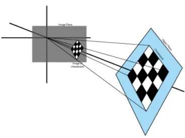
corresponding 3Dspace and image points. The idea is that, given enough correspondences X → x, P may be determined. The usually used method to calibrate a camera, it’s to obtain several images of a known structure in different positions and rotations. A common struc-ture used in camera calibration is the chessboard plan. Basically we move and rotate the chessboard while the camera is taking images. Some other methods use 3D objects (usu-ally covered in markers) with the same purpose without the need to move the object. These methods tend to be harder to work on. Considering the chessboard as the calibration object, from observing a 2D image of it, and knowing that all squares have the same size, we can determine it’s rotation and relative position. This means that we can match x and X and, up to a certain level, know the third coordinate Z in X.
Since we know both x and X, from equation 3.3, x = PX we can determine P. A
rotation matrix can be defined by three angles 3.9 and the translation vector has another three variables giving us six unknown variables. As seen in 3.6, there are four other variables in the intrinsic parameters therefore, making a total of ten values that we have to find so we can define P. At least two images are needed to calibrate a camera, usually, the more you use the better results you get. There are several methods available to find this unknown values. We will analyze the method used in openCV based on Zhang [29, 30] and Borwn[4]. In order to facilitate the comprehension we will, once again, organize the algorithm in steps.
1. Acquire images 2. Chessboard Corners 3. Homography
4. Constraints
5. Closed-form Solution 6. Getting the values
3.2. CAMERA CALIBRATION 23
7. Distortion
The first obvious step of the algorithm is to acquire images to work. These images must be of a chessboard pattern printed in a planar structure and we need at least two. Between frames, we can either move the pattern or the camera. This movement does not need to be known. From each image of the pattern we then extract the chessboard corners.
The following steps will be explained individually in the following sections.
Homography
Figure 3.2: Planar Homography
In computer vision the term homography refers to mapping between points on two image planes. When we haev points in a plane surface and we map them to the image plane we have a homography, hence the need to use a planar surface for the pattern. Again using the notation of X and x, we can express the action of homography as:
x= sHX (3.12)
The importance of using H is that it not only includes the physical transformation but the projection, which includes the camera intrinsic matrix, as well. We can express this by splitting H. Let us define W = [R t] and M = fx 0 cx 0 fy cy 0 0 1 (3.13)
x= sMWX (3.14)
To simplify H we will define Z = 0 therefore allowing us to ignore one column of
R= [r1, r2, r3]. We can now describe the homography by:
H = sM[r1 r2 t] (3.15)
To find H, OpenCv uses multiple images of the same planar pattern. From the previous section we know that for each view there are six unknowns (three angles for rotation and three values for translation). Since we get eight equations from detecting the chessboard we have eight new equations and six unknowns for each view which will allow us to compute H (both intrinsic and extrinsic parameters).
Constraints
From the previous step we collect a homography H for each view. If we write H as column
vectors, H = [h1, h2, h3] we can rewrite equation 3.15 as:
H = [h1 h2h3]= sM[r1r2 t] (3.16) And, considering λ= 1/s: h1 = sMr1 or r1 = λM−1h1 h2 = sMr2 or r2 = λM−1h2 h3= sMt or t = λM−1h 3 (3.17)
Knowing that r1and r2are orthonormal, therefore rT1r2 = 0, we get to our first constraint:
hT1M−TM−1h2= 0 (3.18)
We also know that the rotation vectors have equal magnitude kr1k= kr2k or rT1r1 = rT2r2,
yielding our second constraint:
hT1M−TM−1h1 = hT2M−TM−1h2 (3.19)
We now have two constraints on the intrinsic parameters.
Closed-form solution
In order to make things easier to read and understand we will define B as B = M−TM−1
3.2. CAMERA CALIBRATION 25 B= M−TM−1= B11 B12 B13 B12 B22 B23 B13 B23 B33 (3.20)
Considering the closed-form solution of B we get:
B= 1 fx2 − γ fx2fy cyγ−cxfy fx2fy − γ f2 xfy γ2 f2 xfy2 + 1 f2 y −γ(cyγ−cxfy) f2 xfy2 − cy f2 y cyγ−cxfy f2 xfy −γ(cyγ−cxfy) f2 xfy2 − cy f2 y (cyγ−cxfy)2 f2 xfy2 + c2y f2 y + 1 (3.21)
As mentioned before γ, the skew of the image is almost always equal to 0. Therefore, if we add this new constraint to equation 3.21 we can simplify it’s writing and get:
B= 1 f2 x 0 −cx f2 x 0 f12 y −cy f2 y −cx f2 x − cy f2 y c2x f2 x + c2 y f2 y + 1 (3.22)
From equations 3.20 we can see that B is symmetric, which means we can define it as a
6D vector b= [B11, B12, B22, B13, B23, B33]T. Going back to H, let us define the ithcolumn of
Has hi = [hi1, hi2, hi3] and with this we have:
hTi Bhj = vTi jb (3.23)
Using this definition for vTi j, the two constraints previously defined (equation 3.18 and
3.19) can be rewritten as:
vT 12 (v11− v22)T b= 0 (3.24)
For n images we collect n of these equation which can be stacked in a 2n ∗ 6 matrix V
getting Vb= 0.
Getting the values
Once we have V, from the previous step, we can solve the equation (Vb= 0) for b.
Remem-bering now that b= [B11, B12, B22, B13, B23, B33]Tthe camera intrinsic parameters are directly
calculated from the closed-form solution of B.
fx = pλ/B11 (3.25)
fy =
q
cx = −B13fx2/λ (3.27)
cy = (B12B13− B11B23)/(B11B22− B212) (3.28)
γ = −B12fx2fy/λ (3.29)
λ = B33− (B213+ cy(B12B13− B11B23))/B11 (3.30)
As for the extrinsic values, we compute them from the equation that we read off from the homography condition.
r1 = λM−1h1r2= λM−1h2r3= r1× r2t= λM−1h3 (3.31)
To get an exact rotation matrix, we can not simply join together the r-vectors to form
R = [r1 r2 r3]. If we do this, when using real data, the condition RtR = RRT = 1 will not
hold. To solve this problem we use the SVD of R instead of the original R.
Distortion
We now have all the intrinsic and extrinsic parameters, but no work concerning distortion has yet been done. Cameras have distortion, in more correct words, camera’s lens cause distortion in the image. Distortion makes us "perceive" points on the image in the wrong
place. If we consider (xp, yp), the coordinates of a point, where ’p’ stands for perfect as if
the camera had no distortion, we can also consider (xd, yd) as the point’s distorted location.
With this we can state that:
xp yp = fxXW/ZW + cx fyXW/ZW + cy (3.32)
Using the results of the calibration without distortion: xp yp = (1 + k1 r2+ k2r4+ k3r6) xd yd + 2p1xdyd+ p2(r2+ 2x2d) p1(r2+ 2y2d)+ 2 + p2xdyd (3.33)
To get the distortion parameters a large list of these equations are collected and solved. Once we get the distortion parameters the extrinsic parameters must be re-estimated.
3.2.3
Stereo Cameras
As mentioned before, one way of extracting 3D information from a scene is using stereo cameras. Along with the information about the camera’s intrinsic and extrinsic parameters, we also need to know how to relate the two (more cameras can be used) cameras in the system. Stereo Calibration figure 3.3 is the process of finding a rotation and translation
3.2. CAMERA CALIBRATION 27
matrix that defines the geometrical relationship between the two cameras. In this section we will also talk about Stereo Rectification figure 3.4, which is the process of "making" the cameras optical axes appear parallel. With this, images appear as if they had been taken by cameras with aligned image planes. For these processes the same method of "showing" a calibration is used. Each camera takes, at the same time, an image of the chessboard.
Stereo Calibration
Figure 3.3: Stereo Calibration
So, the objective of stereo calibration is to geometrically relate the cameras but, how can
we do this? We need two matrices, R, the rotation and T the translation. Let us denote TlRl
and TrRr as the rotation and translation matrices, obtained using single-camera calibration,
of the left an right camera respectively. Being P a point in space, in camera coordinates we
get Pl = RlP+ Tl and Pr = RrP+ Tr. Keeping in mind the meaning of R and T in stereo
calibration:
Pl = RT(Pr− T ) (3.34)
If we solve this for R and T :
R= Rr(Rl)TT = Tr− RTl (3.35)
For stereo calibration we use the method described in section 3.2 to get the translation and rotation values of the chessboard and use them in the previous equation. This is done for every view and at each one: errors are introduced due to noise and rounding. To get minimum error values, a Levenberg-Marquardt [19, 25, 21] (LMA) algorithm is used. Starting with a
median of the values of R and F as an initial approximation, the algorithm then finds the minimum of the reprojection error, returning the solution for R and T .
Bouguet’s Algorithm for Stereo Rectification
Figure 3.4: Stereo Rectification
As we will see in the development part of the report, it is easier to work with rectified images. In image 3.4 we can see the objective of image rectification. In OpenCv, two
algorithms are used for image rectification. Hartley’s [12] and Bouguet’s algorithm 1. For
Hartley’s algorithm we simply need to observe points in an image but there is no sense of image scale, furthermore it tends to produce more distorted images. For these reasons and because we can use calibration patterns, we will choose Bouguet’s algorithm.
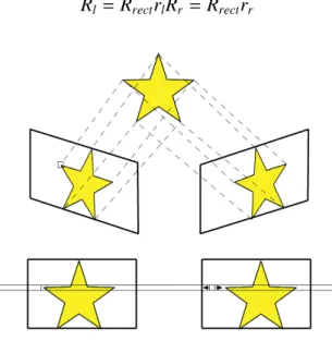
Bouguet’s algorithm works by attempting to minimize of image retro-projection distortion while, at the same time, maximizes common viewing area between the two images. Part of Stereo Rectification is aligning the optical axes. Knowing that we have R that relates
both cameras, if in each camera we apply half a rotation (rrrl for the right and left camera
respectively) we achieve coplanar alignment. To achieve row alignment we need to define
Rrect, we start by defining three vectors:
e1 = T ||T || e2 = [−TyTx0]T q T2 x + Ty2 e3= e1× e2 (3.36)
1Jean-Yves Bouguet never published this algorithm. The algorithm is based in the method presented by
3.3. RECONSTRUCTION 29
Where e2 is orthogonal to e1 and e3 is orthogonal to both e1 and e2. Rrect can now be
defined: Rrect = (e1)T (e2)T (e3)T (3.37)
Rrect will make the epipolar lines horizontal and locates the epipoles at infinity. The
concept of epipolar lines and epipoles will be explained in section 3.3.1. To achieve row alignment, for each camera we have:
Rl = RrectrlRr = Rrectrr (3.38)
Figure 3.5: Rectified Image
Stereo rectification allows us to find the rectification maps which, when applied to im-ages, aligns them. When we say that the images are aligned we mean that the rows of pixels between the two cameras are aligned as we can see in figure 3.5. It is easily understood the advantages that this brings. Having to find the same point in two images we can restrict the search to a row of pixels instead of searching in the entire image. With this we can increase efficiency and, by restricting the points that are possible matches, we also increase reliability.
3.3
Reconstruction
3.3.1
Epipolar Geometry
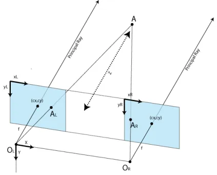
When a scene is viewed from two different cameras every point of the scene will have dif-ferent projections in each image plane. In fig3.6 we have two cameras with their respective
Figure 3.6: Epipolar geometry
planes is denoted xL and xR. The line connecting both focal points is called baseline and
its intersection with the images planes creates eL and eR which are the epipoles. The plane
defined by the baseline and point X is called the epipolar plane. The line that contains a projection and an epipolar point on the same image is called an epipolar line. The epipolar geometry of a scene can be defined by a matrix called Fundamental Matrix (F). This matrix depends only on the relative position of the cameras.
x0TF x= 0 (3.39)
Eq3.39 defines the relation between the two cameras and the projected points. If the equation
is confirmed, the point xLbelongs to the left view epipolar line that corresponds to projection
point xR. Note that a null result is not enough to say that xLand xR are projections from the
same point in the scene. As we can see from Fig3.6 three example points (X1,X2 and X3) will all have a null result in Eq3.39 even though they are different points in the scene.
3.3.2
Fundamental matrix
The fundamental matrix [24] [11] is a 3 × 3 matrix with rank 2 and 7 degrees of freedom.
Even though there are 9 elements, scaling is not significant and DetF = 0 removing one
degree of freedom. There are two different ways of finding the Fundamental Matrix, we can either find it from known camera matrices or compute it from point correspondences. In single camera systems we will be using only one camera which can be calibrated. However, even if we calibrate the camera we can only use the intrinsic parameters. A camera matrix is composed of intrinsic and extrinsic parameters, using a moving camera makes the use of the same extrinsic parameters throughout the process impossible. For this reason we will rely on
3.3. RECONSTRUCTION 31
extracting the camera matrices from the fundamental matrix, which in turn will be extracted from point correspondences. To extract the fundamental matrix from camera matrices we use the following:
F = [e0]xP0P+ (3.40)
Equation Eq3.40 will give the fundamental matrix from two known camera matrices where
e0 is the epipole of camera P0, [e0]x is the skew-simetric correspondence of e0 and P+ is the
pseudoinverseof P.
If camera matrices are not known we can compute F from point correspondences between the images. If there is only one camera this is the most effective way to extract 3D information from a scene. We can also predict where the camera is after a certain movement and define it as the second camera. Predicting where the camera will be after a certain movement is not accurate for various reasons such as unpredicted variations on the floor. The procedure of estimating the intrinsic parameters of two unknown cameras from point correspondence is known as structure from motion [11, ?]. Starting with eq 3.39 for any pair of corresponding
points xiand Xi0in the two images we get:
x0x f11+ x0y f12+ x0f13+ y0x f21+ y0y f22+ y0f23+ x f31+ y f32+ f33 = 0 (3.41)
For n pairs of points we have:
A f = x0 1x1 x 0 1y1 x 0 1 y 0 1x1 y 0 1 x1 y1 1 ... ... ... ... ... ... ... ... x0nxn x0nyn x0n y 0 1xn y0n xn yn 1 f = 0 (3.42)
Because F has only 7 degrees of freedom only 7 pairs of points are needed to find a
solution however 8 pairs are usually used. Solving the equation system A f = 0 we can get
F. Most of the times more than 8 points are used and each extra point originates an extra line in matrix A. If we have more points than variables in an equation system, the system is said to be over-determined. In most of the cases there is no single solution and for that we must find the one which minimizes the error. The most commonly used methods of solving such equation systems are the RANSAC algorithm [7] and the SVD method [28].
The Ransac (RANdom SAmple Consensus) algorithm is a method to estimate parame-ters of a mathematical model designed to cope with a large proportion of outliers in the input data, which normally happens when extracting 3D information from a scene. RANSAC is an iterative method choosing in each iteration a random minimum number of points required to solve the model. After solving the model with the chosen points it will determine how
many of the remaining points are consistent with the model. If the number of consistent points is enough (determined with a given tolerance) the model will be re-estimated using all consistent points and terminates. If the number isn’t enough a new sample of points will be randomly chosen and following steps repeated.
The SVD (Singular Value Decomposition) method is a commonly used method for
solv-ing matrix equations of the type Ax= 0. The method starts by separating the original matrix
Ain three matrices A= UDVT. D is a diagonal matrix containing the singular values of A.
U and V are orthogonal matrices where V contains the singular vectors of the correspondent
to the singular values of D. When the method is applied to A, the last column of resulting V will correspond to a minimizing solution of f . With f the matrix F can then be built.
3.3.3
Reconstruction
Triangulation, sometimes also referred as reconstruction, is the method of finding a point in a 3D space given at least two projections of the same point in images. The work-flow of 3D reconstruction is the following:
1. Find points 2. Match points
3. Fundamental matrix F
4. From F compute PA and PB
5. Compute X in the world for each x and x0matching pair.
Up to this point, steps 1, 2 and 3 were already explained and, in the previous section we, explained that the camera matrices can be either extracted from the fundamental matrix or built from known camera parameters. Now we will show how to extract camera matrices from the F as well as how to triangulate a point.
Camera matrices
The fundamental matrix encodes information of both the intrinsic and extrinsic parameters
of the cameras. Let us start by defining PA and PB as the camera’s projection matrices and
remembering the basic form of a camera matrix:
3.3. RECONSTRUCTION 33
Now let us consider that PA is in the origin of the world coordinates, meaning that t =
[0, 0, 0]T, and that P
A’s focal length= 1. With this we can write 3.43 for PA as:
P= [I|0] (3.44)
Then, because:
x0TF x= XTPPFPAX (3.45)
and:
PTBFPA = [S F|e0]TF[I|0] (3.46)
Where e0 is the epipole and S a skew-symmetric matrix, we can say that:
PB = [S F|e0] (3.47)
A good choice for S is S = [e0], which means that we can once again rewrite P
Bas
PB= [[e0]F|e0] (3.48)
All we need now is to find the epipoles from F. Two of the properties of F is that Fe1= 0
and eT
2F = 0. Using SVD we can easily calculate the epipoles.
Triangulation
In image fig3.6 we can see that point X is the intersection of the lines that start in OL and
OR and pass through XL and XR respectively. These lines are called projection lines. This
intersection along with both focal points creates a triangle which is the base for triangulation. In theory these lines should always intersect however for various reasons such as camera dis-tortion this intersection can never happen. If the lines did intersect, finding an intersection in space between two lines is a trivial procedure.However an intersection, in most cases, won’t be found. Different triangulation methods deal with this problem differently [13].
The common method to deal with the problem of non-intersecting lines is the Mid-Point method [3], which as the name suggests will choose the middle point of the smallest line connecting both projection lines. This method will not give the best results since a lot of approximations are made. Other methods [13, 15] are based in moving the corresponding pixels of the point’s projection point so that the projection lines intersect. Such methods are called optimal correction methods. The main goal of these methods is to minimize 3.39. For an optimal solution the movement of the pixels must be the minimum needed i.e. min-imizing the error given by the squared sum of the movements. While in [13] the error is minimized by solving a grade 6 polynomial, [16] chooses a different approach that can be