Modeling and mapping basal area of Pinus taeda L. plantation using airborne LiDAR data

Printed version ISSN 0001-3765 / Online version ISSN 1678-2690 http://dx.doi.org/10.1590/0001-3765201720160324

www.scielo.br/aabc | www.fb.com/aabcjournal

Modeling and mapping basal area of

Pinus taeda

_{L. plantation using airborne LiDAR data}

CARLOS A. SILVA1, 2

, CARINE KLAUBERG2

, ANDREW T. HUDAK2

, LEE A. VIERLING1, SCOTT J. FENNEMA3 and ANA PAULA D. CORTE4

1

Department of Natural Resources and Society, College of Natural Resources, University of Idaho/UI, 875 Perimeter Drive, Moscow, 83843 Idaho, USA

2

USDA Forest Service, Rocky Mountain Research Station, RMRS, 1221 South Main Street, Moscow, 83843 Idaho, USA 3

Water Resources Program, College of Agriculture and Life Sciences, University of Idaho, Moscow, 83844 Idaho, USA 4

Departamento de Engenharia Florestal, Universidade Federal do Paraná, Avenida Prefeito Lothário Meissner, 900, Jardim Botânico, 80210-170 Curitiba, PR, Brazil

Manuscript received on June 1, 2016; accepted for publication on April 25, 2017

ABSTRACT

Basal area (BA) is a good predictor of timber stand volume and forest growth. This study developed predictive models using field and airborne LiDAR (Light Detection and Ranging) data for estimation of basal area in Pinus taeda plantation in south Brazil. In the field, BA was collected from conventional forest inventory plots. Multiple linear regression models for predicting BA from LiDAR-derived metrics were developed and evaluated for predictive power and parsimony. The best model to predict BA from a family of six models was selected based on corrected Akaike Information Criterion (AICc) and assessed by the adjusted coefficient of determination (adj. R²) and root mean square error (RMSE). The best model revealed an adj. R²=0.93 and RMSE=7.74%. Leave one out cross-validation of the best regression model was also computed, and revealed an adj. R² and RMSE of 0.92 and 8.31%, respectively. This study showed that LiDAR-derived metrics can be used to predict BA in Pinus taeda plantations in south Brazil with high precision. We conclude that there is good potential to monitor growth in this type of plantations using airborne LiDAR. We hope that the promising results for BA modeling presented herein will stimulate to operate this technology in Brazil.

Key words: Forest Inventory, LiDAR metrics, Multiple Linear Regression, Remote Sensing.

Correspondence to: Carlos Alberto Silva

E-mail: carlos_engflorestal@outlook.com

INTRODUCTION

In Brazil, pine plantations cover 1.59 million

hectares, and are the most important long fiber

source for pulp and paper production—accounting for approximately 20.54% of the country’s total reforested area (Ibá 2015). Most of the pine

plantations are concentrated in south Brazil, with 34.1 and 42.4% of the total reforested area located in Paraná and Santa Catarina states (Ibá 2015). Pinus

taeda L., whose common name is loblolly pine, is

extremely valuable since it is the most planted tree species in the region (Kohler et al. 2014).

conditions during initial growth stages, and determine optimal harvest time. Inventories measure tree diameter and basal area. Basal area describes the state of the stand and it aids directly the thinning decisions (Reukema 1975, Emmingham and Green 2003). Diameter and basal area distributions are therefore used in many forest management planning packages for predicting stand volume and growth (Gobakken and Næsset 2004). The most accurate method of estimating basal area in loblolly pine plantations is to physically sample it in the field. However, field measurements of forest attributes over large areas are limited by budgets and time, making them impractical (Hummel et al. 2011, Silva et al. 2014).

Light Detection and Ranging (LiDAR), is a powerful and well-suited technology for mapping many forest attributes, including basal area. LiDAR is very useful for providing high resolution, three-dimensional information of vertical and horizontal forest structures and the underlying topography (Silva et al. 2016a). In forestry, key LiDAR applications include high accuracy retrieval of tree density, stem volume, above ground carbon, leaf area index and basal area (e.g. Næsset and Bjerknes 2001, Andersen et al. 2005, Hudak et al. 2006, Silva et al. 2014). LiDAR has been widely used to quantify and map forest attributes in conifer and deciduous forests types (e.g., Næsset 1997, Næsset and Bjerknes 2001, Popescu et al. 2003, Popescu 2007). However, in Brazil LiDAR has not been widely used to predict forest attributes in pine plantations as it has been used to predict and map forest attributes in Eucalyptusplantations (e.g., Silva et al. 2014, 2016a, 2017, Carvalho et al. 2015).

In many countries, LiDAR has already moved from the research arena to operational reality in the area of forest resource inventory. In Brazil, the use of LiDAR for predicting forest inventory is still really new and therefore requires more research to test and validate this technology in Brazilians

pine forest plantations. Thus far only Zandoná et al. (2008) and Müller et al. (2014) have used airborne LiDAR data for forest inventory purposes in loblolly pine plantations in south Brazil.

This study was designed to test the accuracy of LiDAR-based approach to quantify BA in P. taeda plantation, in southern Brazil. The specific

aims were to: i) determine which LiDAR-derived metrics are most useful to predict BA; ii) derive, test and select the best model for predicting BA; and iii) apply the best model across the landscape to map the spatial distribution of BA at the stand-level.

MATERIALS AND METHODS

STUDY AREA DESCRIPTION

The study area consisted of four P. taeda plantations located within the Telêmaco Borba municipality in the state of Paraná, Southern Region of Brazil (Fig. 1). The climate of the region is characterized as warm and temperate (Cfa) (Köppen and Geiger 1928), with mean annual precipitation of 1378 mm and the mean annual temperature of 18.4º C. The regions topography is complex, ranging from 618 m to 905 m. The plantations are managed by Klabin Celulose S/A, a pulp company, and all the trees were planted evenly along a 2.5 x 2.5 m or 3.0 x 2.0 m grid configuration, resulting in a mean tree density of 1,600 and 1,667 trees per ha, respectively.

FIELD DATA COLLECTION

total basal area (BA; m2 ha-1) was then calculated for each sample plot using the following the equation:

BA_n (m2 ha-1)

2 i

ð*DBH

40000 *10000 PA

=

∑

Where: BA_n is basal area in m2 ha-1 for the plot n; DBH is the diameter at breast height (1.30 m) in cm for tree i; PA is plot area in m2_{. Summary statistics} of BA per stand ages are presented in Table I.

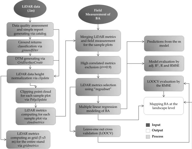
LIDAR DATA ACQUISITION AND PROCESSING LiDAR data were obtained using a Harrier 68i sensor mounted on a CESSNA 206 aircraft. Table II describes the characteristics and precision of the LiDAR data. LiDAR data processing consisted of several steps that ingested the LiDAR point cloud data and provided two major outputs: the digital terrain model (DTM), and the

LiDAR-derived canopy structure metrics. All of the LiDAR processing was performed using the US Forest Service FUSION/LDV 3.42 software toolkit (McGaughey 2015).

measured sample plots, and the CloudMetrics tool was applied to compute the LiDAR-derived metrics using all the available returns of the point cloud. Finally, the GridMetrics function was used to generate the same LiDAR metrics as computed with CloudMetrics, but now within grid cells of 25 m spatial resolution across the landscape. The list of the LiDAR metrics computed in this are presented in the Table III.

MODELING DEVELOPMENT AND ASSESSMENT Pearson’s correlation (r) was used to identify highly correlated predictor variables (r>0.9); redundant predictors were subsequently excluded to help guard against overfitting the predictive model. We determined the best LiDAR metrics using the regsubsets function in the Leaps package in R (R Development Core Team 2015), which selects the best subset of predictor variables using the Mallows Cp statistic (Mallows 1973). We then used the Lm linear model function in R to define the prospective

linear regression models. To measure the quality of each model, the corrected Akaike information criterion (AICc) (Akaike 1973, 1974) was calculated and ranked accordingly by minimum AIC. Model ranking was done using AICc since we had small sample size (n/p < 40, where n is number of samples and p is number of parameters of the model) (Hurvich and Tsai 1989). Residuals from all prospective models were analyzed graphically and tested for normality using the Shapiro-Wilk test (Shapiro and Wilk 1965) and for heteroscedasticity using the Breusch-Pagan test (Breusch and Pagan 1979).

BA was positively skewed, causing poor model fits at the tails of a distribution because ordinary least squares (OLS) regression assumes a normal distribution in the response variable. Therefore, natural logarithm (ln) transforms were applied to the response variable before modeling. The final BA prediction on the natural scale was obtained by multiplying the output prediction by the correction factor of exp (0.5 x MSE), were MSE is the mean square error of the residuals. The precision of the model predictions were then evaluated in terms of Person’s correlation (r; eq.2), adjusted coefficient of determination (adj.R²; eq.3 and 4), and Root Mean Square Error (RMSE; eq.5 and 6), both absolute (m2 ha-1) and relative (%):

(

)(

)

(

)

(

)

n

i i

i 1

n 2 n 2

i i

i 1 i 1

x x y y r

x x y y

=

= =

− −

=

− −

∑

∑

∑

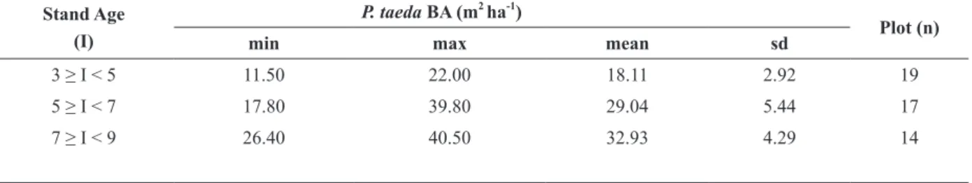
TABLE I

Characteristics of the study plots. Basal Area (BA) values are based on in-situ measured sample plots (n=50). Stand Age

(I)

P. taeda _{BA (m}2 ha-1

)

Plot (n)

min max mean sd

3 ≥ I < 5 11.50 22.00 18.11 2.92 19

5 ≥ I < 7 17.80 39.80 29.04 5.44 17

7 ≥ I < 9 26.40 40.50 32.93 4.29 14

TABLE II

LiDAR flight characteristics.

Parameter Value

Scan angle (°) off nadir 30º

Footprint (m) 0.33m

Flight speed (km/h) 234 km/h

Horizontal accuracy 10cm

Elevation accuracy 15cm

Operating altitude 666 m

Scan frequency 300 kHz

(

)

n ₂

i

2 i 1

n ₂ n 2 i 1 i

i i 1

y

R

1

y

y

x

n

−

= −

−

∑

∑

∑

(

)

2 2

n 1

adj.R

1

1

n

p 1

R



−



= − −

_

_

− −





(

)

(

)

n

− ₌

∑

( )

(

)

n 2

i i

i 1 x y

n

RMSE % *100

x

= −

=

∑

(6)

Where n is the number of plots, is the observed value for plot i, and is the predicted value for plot i, and are the mean of the observed and predicted BA values, p is the number of independent variables. Statistical equivalence tests were employed (Robinson 2015) to assess whether the predicted BA is statistically similar (i.e., equivalent) to the field-based, observed BA. We defined an acceptable accuracy as a relative RMSE below 15%. Based on the AICc values, the best model was selected and evaluated by means of a leave-one-out cross-validation – LOOCV strategy. We used the yaImpute package in R (Crookston and Finley 2008) to apply the best model across the landscape to map the spatial distribution of BA of P. taeda at the stand level. An overview of the methodology is outlined in Fig. 2.

RESULTS

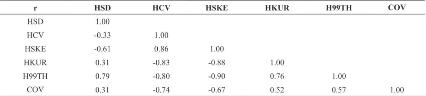
According to Pearson’s correlation (r), 24 (80%) of the LiDAR-derived metrics were highly correlated (r>0.9). The remaining six metrics not highly correlated were HSD, HCV, HSKE, HKUR, H99TH and COV. Even though the number of metrics was greatly reduced, these metrics still represented the canopy height (e.g., H99TH), cover (COV) and

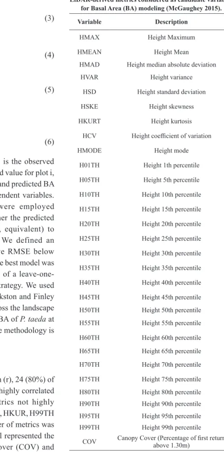
TABLE III

LiDAR-derived metrics considered as candidate variables for Basal Area (BA) modeling (McGaughey 2015).

Variable Description

HMAX Height Maximum

HMEAN Height Mean

HMAD Height median absolute deviation

HVAR Height variance

HSD Height standard deviation

HSKE Height skewness

HKURT Height kurtosis

HCV Height coefficient of variation

HMODE Height mode

H01TH Height 1th percentile

H05TH Height 5th percentile

H10TH Height 10th percentile

H15TH Height 15th percentile H20TH Height 20th percentile

H25TH Height 25th percentile

H30TH Height 30th percentile

H35TH Height 35th percentile H40TH Height 40th percentile

H45TH Height 45th percentile H50TH Height 50th percentile H55TH Height 55th percentile

H60TH Height 60th percentile H65TH Height 65th percentile H70TH Height 70th percentile

H75TH Height 75th percentile H80TH Height 80th percentile H90TH Height 90th percentile H95TH Height 95th percentile H99TH Height 99th percentile

variation (HCV). Table IV summarizes the Pearson statistics.

The best metrics ranked according to the regsubset for predicting BA were H99TH, HCV, COV, HSKE, HKUR. Table V shows the competing models and diagnostic statistics for predicting plot-level BA from LiDAR-derived metrics. Six best subset models were developed, and for these models the adj.R² ranged from 0.84 to 0.97. The AICc ranged from -108.67 to -67.30, absolute RMSE ranged from 1.96 to 3.04 m2 _ha-1_{, and} relative RMSE ranged from 7.54 to 11.71%.

We observed that the inclusion of more than three metrics did not improve the model fit significantly. Therefore, the best model according

Breusch-Pagan tests were 0.98 (p =0.45) and 0.08 (p =0.78), respectively.

The MSE (0.005) for best BA model was substituted in the correction factor equation and the predicited BA was multiplied by the computed

correction factor of 1.002 to converted the predicions from natural-logarithm-transformed

scale to natural scale. Thus , the predicted BA of P. taeda for the 50 sample plots in this study ranged

from 13.43 to 39.13 m2 ha-1 (Fig. 4). Moreover, the

selected best model was applied across the extent of the study area to map the BA at the landscape

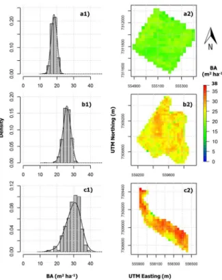
level. Fig. 5 shows the spatial distribution of the predicted BA for three stands with ages ranging

from 4 to 8 years old. Predicted BA (m2 ha-1) on

natural scale per hectare for stands A, B and C

were approximately 17.59 (± 2.37); 24.87 (± 3.59); 28.48 (± 5.68) m2 ha-1, respectively.

DISCUSSION

LiDAR is an important forest inventory data

source when combined with appropriately designed sample plots in the field and with appropriate modeling tools (Hudak et al. 2006), and even though LiDAR data have been used widely for forest inventory (Næsset 1997, Maltamo et al. 2004, Hudak et al. 2006, 2014, Silva et al. 2016b), this is the first time that airborne LiDARhas been applied to predict and map basal area at plot- and landscape-levels pine plantations of south Brazil.

LiDAR is increasingly being used as a means

for obtaining forest structural measurements over TABLE IV

Pearson’s correlation matrix among LiDAR metrics selected.

r HSD HCV HSKE HKUR H99TH COV

HSD 1.00

HCV -0.33 1.00

HSKE -0.61 0.86 1.00

HKUR 0.31 -0.83 -0.88 1.00

H99TH 0.79 -0.80 -0.90 0.76 1.00

COV 0.31 -0.74 -0.67 0.52 0.57 1.00

TABLE V

LiDAR-derived models for predicting BA (natural-logarithm transformed) in P. taeda _{plantations. Pearson’s correlation}

(r), Adjusted coefficients of determination (adj.R²), root mean square error (RMSE) and corrected Akaike information

criterion (AICc). Bold values represent the best model.

Model LiDAR derived metrics r Adj.R² RMSE AIC

m2

ha-1 _%

1 2.04 + 0.12* H99TH 0.84 0.92 3.04 11.71 -67.30

2 2.97 + 0.08* H99TH - 2.21 HCV 0.96 0.92 2.12 8.18 -97.13

Figure 4 - Observed versus predicted BA (natural scale) from the best model and LOOCV

across plantation ages for the sample plots (n=50).

Figure 3 - a) Observed versus predicted BA (natural scale) from the adjusted model; b) Observed versus predicted BA from

LOOCV; (n=50). The grey polygon represents the ± 25% region of equivalence for the intercept, and the black vertical bar represents a 95% of confidence interval for the intercept. The predicted BA from model and LOOCV are equivalents to the

field-based BA for the intercept if the black vertical bar is completely within the grey polygon. If the grey polygon is lower than the black vertical bar, the predicted BA is biased low; and if it is higher than the black vertical bar, the predicted BA is biased high.

The grey dashed line represents the ± 25% region of equivalence for the slope, and if the solid black line is contained completely within the grey dashed line, the pairwise measurements are equal. A bar that is wider than the region outlined by the grey dashed lines indicates highly variable predictions. The white dots are the pairwise measurements, and the solid black line is a best-fit linear

large areas, and many LiDAR metrics can be used as candidates for predicting forest structure attributes (Hyyppa et al. 2008, Wulder et al. 2008, Van Leeuwen and Nieuwenhuis 2012, Treiz et al. 2012, Silva et al. 2014). In the P. taeda plantation environment due the homogeneity of canopy structure, we observed that most of LiDAR-derived metrics have been identified as highly correlated.

In this study, due the high homogeneity of this type of plantation, H99TH, HCV and COV provided accurate predictions of BA. These metrics most efficiently described the canopy structure of the forest, by capturing the majority of canopy structure variation. Although we selected just three variables to assess BA, the most important and number of metrics to include in the LiDAR-derived model will also depend on forest type and the variability of the response variable. For instance, Holmgren (2004) also included other LiDAR-derived metrics, such as H99TH and COV, in a BA predicting model for a mixed forest in south-western Sweden. On the other hand, Hudak et al. (2006) used both LiDAR and image-derived metrics to predict BA in mixed forests located in north-central Idaho, USA.

Although the cost of LiDAR data acquisition was not a central objective in this study, it is nonetheless an important factor to consider. The acquisition cost of LiDAR data is still high, especially in Brazil where the there are few vendors. However,LiDAR offers opportunities for rapidly estimating forest attributes, such as BA, over extensive areas with high accuracy (Hummel et al. 2011), and greatly reduces the amount of time and effort required for field-based measurements. In this study, we predicted and mapped BA at the landscape level at a spatial resolution of 25 m and with RMSE at plot-level lower than the 15% established in the materials and methods. In the Figure 5, we presented some of the basal area maps generated from the best LiDAR-derived model. The spatial distribution and variability of BA at stand level was not evaluated in this study,

however, differences in BA at stand level may be related to topography, age and management practices of forest stands. Moreover, differences in BA may also depend on other factors such as i) type and intensity of land use before the establishment of a forest stand, ii) amount of soil compaction and reduction of soils fertility (Parker et al. 2007), iii) genetic variability (Emhart et al. 2006); iv) plant stress due high stand density (Sharma 2013), which could be described as competition index (Rivas et al. 2005, Uzoh and Oliver 2008) and v) site index.

CONCLUSIONS

This study presented a simplified framework for predicting and mapping BA of P. taeda plantations

using airborne LiDAR data. The most useful LiDAR metrics for assessing BA were H99TH, HCV and COV. The best model showed high accuracy for predicting BA with overall RMSE less than 10%. High spatial resolution maps of BA were created from the LiDAR data once a robust model was developed. We conclude that this LiDAR-based approach is capable of providing suitably accuracy estimates of BA at plot and stand-levels for operational use in inventories of south pine plantations in southern Brazil. We hope that the promising results for forest inventory modeling presented herein will stimulate to operational use of this technology in Brazil.

ACKNOWLEDGMENTS

This research was funded through a Ph.D scholarship from the Conselho Nacional de Desenvolvimento Científico e Tecnológico (CNPq) via the Brazilian Science without Borders program (249802/2013-9). The authors are very grateful for the LiDAR and field inventory data collections funded by Klabin S.A, a Brazilian pulp and paper company. We thank Luiz Gastão Bernett, Clewerson Frederico Scheraiber and Emerson Roberto Schoeninger for their helpful contribution on field data collection. Finally, we thank the anonymous reviewers for the helpful suggestions on an earlier draft of the manuscript.

REFERENCES

ANDERSEN H, MCGAUGHEY RJ AND REUTEBUCH

SE. 2005 Estimating forest canopy fuel parameters using LIDAR data. Remote Sensing Environ 94: 441-449.

AKAIKE H. 1973. Information theory and an extension of the

maximum likelihood principle. In: Proceedings of the 2nd International Symposium on Information Theory. Petrov BN and Csake F (Eds) Akademiai Kiado, p. 267-281.

AKAIKE H. 1974. A new look at the statistical model

identification. IEEE Trans Autom Control 19: 716-723.

BREUSCH TS AND PAGAN AR. 1979. A simple test for

heteroscedasticity and random coefficient variation. Econometrica 47: 1287-1294.

CARVALHO SPC, RODRIGUEZ LCE, SILVA LD, CARVALHO LMT, CALEGARIO N, LIMA MP, SILVA

CA, MENDONÇA AR AND NICOLETTI MF. 2015. Predição do volume de árvores integrando LiDAR e Geoestatística. Scien For 43: 627-637.

CROOKSTON NL AND FINLEY AO. 2008. YaImpute: An R Package for kNN Imputation. J Stat Soft 23: 1-16.

EMHART IV, MARTIN TA, WHITE TL AND HUBER DA.

2006. Genetic variation in basal area increment phenology and its correlation with growth rate in loblolly and slash pine families and clones. Can J For Res 36: 961-971.

EMMINGHAM WH AND GREEN D. 2003. The Woodland

Workbook. In: Thinning systems for western Oregon Douglas-fir stands EC1132. Corvallis, OR, USA: Oregon State University.

GOBAKKEN T AND NÆSSET E. 2004. Estimation of diameter and basal area distributions in coniferous forest by means of airborne laser scanner data. Scand J For Res 19: 529-542

HOLMGREN J. 2004. Prediction of Tree Height, Basal Area

and Stem Volume in Forest Stands Using Airborne Laser Scanning. Scand J For Res 19: 543-553.

HUDAK AT, CROOKSTON NL, EVANS JS, FALKOWSKI MJ, SMITH AMS AND GESSLER PE. 2006. Regression

modeling and mapping of coniferous forest basal area and tree density from discrete-return LiDAR and multispectral satellite data. Can J Remote Sens 32: 126-138.

HUMMEL S, HUDAK AT, UEBLER EH, FALKOWSKI MJ

AND MEGOWN KA. 2011. A comparison of accuracy and cost of LiDAR versus stand exam data for landscape management on the Malheur National Forest. J For 109: 267-273.

HURVICH CM AND TSAI CL. 1989. Regression and time

series model selection in small samples. Biometrika 76: 297-307.

HYYPPA J, HYYPPA H, LECKIE D, GOUGEON F, YU X

AND MALTAMO M. 2008 Review of methods of small-footprint airbone laser scanning for extracting forest inventory data in boreal forests. Int J Remote Sens 29: 1339-1366.

IBÁ. 2015. Brazilian Tree Industry. Brasilia: IBÁ, 80 p. http:// www.iba.org/images/shar ed/iba_2015.pdf/

KOHLER SV, WOLFF N I, FILHO AF AND ARCE JE. 2014.

Dinâmica do sortimento de plantios de Pinus taeda L. em diferentes classes de sítio no Sul do Brasil. Scien For 42: 403-410.

KÖPPEN W AND GEIGER R. 1928. Klimate der Erde. Gotha: Verlag Justus Perthes. Wall-map 150cm×200cm.

KRAUS K AND PFEIFER N. 1998. Determination of terrain models in wooded areas with airborne laser scanner data. ISPRS J Photogramm Remote Sens 53: 3193-3203. MALLOWS CL. 1973. Some comments on Cp. Technometrics,

MALTAMO M, EERIKÄINEN K, PITKÄNEN J, HYYPPÄ J AND VEHMAS M. 2004. Estimation of timber volume

and stem density based on scanning laser altimetry and expected tree size distribution functions. Remote Sens Environ 90: 319-330.

MCGAUGHEY RJ. 2015. FUSION/LDV: software for LiDAR

Data Analysis and Visualization [Computer program]. Washington: USDA, Forest Service Pacific Northwest Research Station, http://http://forsys.cfr.washington.edu/ fusion/ FUSION_manual. pdf/

MÜLLER M, KERSTING APB, NAKAJIMA NY,

HOSOKAWA RT AND ROSOT NC. 2014. Influence

of flight configuration used for LiDAR data collection on individual trees data extraction in forest plantations. Floresta, Curitiba, PR 44: 279-290.

NÆSSET E. 1997. Determination of mean tree height of forest stands using airborne laser scanner data. ISPRS J Photogramm. Remote Sens 52: 49-56.

NÆSSET E AND BJERKNES KO. 2001. Estimating tree heights and number of stems in young forest stands using airborne laser scanner data. Remote Sens Environ 78: 328-340.

PARKER RT, MAGUIRE DA, MARSHALL DD AND COCHRAN P. 2007. Ponderosa Pine Growth Response to

Soil Strength in the Volcanic Ash Soils of Central Oregon. West J Appl For 22: 134-141.

POPESCU SC. 2007. Estimating biomass of individual pine trees using airborne LiDAR. Biomass and Bioenergy 31: 646-655.

POPESCU SC, WYNNE RH AND NELSON RF. 2003.

Measuring individual tree crown diameter with LiDAR and assessing its influence on estimating forest volume and biomass. Can J Remote Sens 29: 564-577.

R DEVELOPMENT CORE TEAM. 2015. R: A language and environment for statistical computing. Vienna: R Foundation for Statistical Computing. http://www.r-project.org/

REUKEMA DL. 1975. USDA Forest Service General Technical Report PNW. In Guidelines for precommercial thinning of Douglas-fir. Volume 30. Portland, OR, USA: United States Department of Agriculture.

RIVAS JJC, GONZALEZ JGA, AGUIRRE O AND

HERNANDEZ F. 2005. The effect of competition on

individual tree basal area growth in mature stands of Pinus cooperi Blanco in Durango (Mexico). European Journal of Forest Research 124: 133-142.

ROBINSON A. 2015. Equivalence: Provides Tests and Graphics for Assessing Tests of Equivalence, Version 0.7.2. https://cran.r-project.org/web/packages/equivalence/.

SHARMA RP. 2013. Modelling height, height growth and

site index from national forest inventory data in Norway. Norwegian University of Life Sciences, Norway, 172 p.

SILVA CA, HUDAK AT, KLAUBERG C, VIERLING LA, GONZALEZ-BENECKE C, CARVALHO SPC,

RODRIGUEZ LCE, AND CARDIL A. 2017. Combined effect of pulse density and grid cell size on predicting and mapping aboveground carbon in fast-growing Eucalyptus forest plantation using airborne LiDAR data. Carbon Balance and Management 12: 1-16.

SILVA CA, HUDAK AT, VIERLING LA, LOUDERMILK EL, O’BRIEN JJ, HIERS K, JACK SB, GONZALEZ-BENECKE C, LEE H, FALKOWSKI MJ AND KHOSRAVIPOUR A. 2016b. Imputation of individual

Longleaf Pine (Pinus palustris Mill.) Tree attributes from field and LiDAR data. In: Canadian Journal of Remote Sensing 42: 554-573.

SILVA CA, KLAUBERG C, CARVALHO SPC, HUDAK AT

AND RODRIGUEZ LCE. 2014. Mapping aboveground carbon stocks using LiDAR data in Eucalyptus spp. plantations in the state of São Paulo, Brazil. Scien For 42: 591-604.

SILVA CA, KLAUBERG C, HUDAK AT, VIERLING LA, LIESENBERG V, CARVALHO SPC AND RODRIGUEZ

LCE. 2016a. A principal component approach for predicting the stem volume in Eucalyptus plantations in Brazil using airborne LiDAR data. Forestry 2016 84: 422-433.

SHAPIRO SS AND WILK MB. 1965. An analysis of variance

test for normality (complete samples). Biometrika 52: 591-611.

TREIZ P, LIM K, WOODS M, PITT D, NESBITT D AND

ETHERIDGE D. 2012. LiDAR Sampling Density for

Forest Resource Inventories in Ontario, Canada. Remote Sens 4: 830-848.

UZOH FCC AND OLIVER WW. 2006. Individual tree

height increment model for managed even-aged stands of ponderosa pine throughout the western United States using linear mixed effects models. For Eco and Man 221: 147-154.

VAN LEEUWEN M AND NIEUWENHUIS M. 2012.

Retrieval of forest structural parameters using LiDAR remote sensing. Eur J For Res 129: 749-770.

WULDER MA, BATER CW, COOPS NC, HILKER T AND WHITE JC. 2008. The role of LiDAR in sustainable forest

management. Forest Chron 84: 807-826.