Vol.49, Special : pp. 87-95, January 2006
ISSN 1516-8913 Printed in Brazil BRAZILIAN ARCHIVES OF
BIOLOGY AND TECHNOLOGY
A N I N T E R N A T I O N A L J O U R N A L
Uncertainty of the Density of Moist Air: Gum x Monte Carlo
Moacyr Canaves Junior∗ and Pedro José Pompéia
Instituto de Fomento e Coordenação Industrial (IFI); Centro Técnico Aeroespacial (CTA); pedro.pompeia@ifi.cta.br; moacyr.canavesjr@ifi.cta.br; Praça Marechal do Ar Eduardo Gomes, 50; 12.228-904; São José dos Campos - SP - Brasil
ABSTRACT
In this study two methods of evaluation of uncertainty, the law of propagation of uncertainties (as recommended by GUM) and the method of Monte Carlo, are compared. As a particular case the determination of the density of moist air was considered The results show that there are some differences between both methods.
Key words: Density of moist air, propagation of uncertainties, Monte Carlo
∗
INTRODUCTION
As it is well known by metrologists, “a complete expression of the result of a measurement includes
information about the uncertainty of
measurement.” (Inmetro, 1995). It is also true that, “ with the aim to establish criterions and general rules, as to harmonize methods and procedures related to the expression of uncertainties associated with the processes of measurements”, the Guide to the Expression of Uncertainty of Measurement (GUM, 2003) was published and it contains the recommendations for a correct evaluation of uncertainty in measurement.
This reference has really played its role and has been widely used in most laboratories with metrological aims. In GUM (2003), the method to evaluate the uncertainty of measurement makes use of the “law of propagation of uncertainties”. However, as every method that is intended to solve a problem, GUM also has its limitations.
An alternative way to evaluate the uncertainty in measurement has been recently studied (Moscati et
al.,2004) and successfully applied in some cases
(Reis et al., 2004) and makes use of computational simulations with the method of Monte Carlo. With this method, in which the probability distributions are propagated, some limitations of the method of the GUM are avoided. This has motivated the elaboration of a supplement to GUM, that is still in discussion among a restricted group of specialists (Moscati et al., 2004).
EVALUATION OF UNCERTAINTY ACCORDING TO GUM AND THE DENSITY OF MOIST AIR
Recommendations of GUM
According to GUM, when one cannot realize a
direct measurement of a measurand Y, a
mathematical model must be searched, which allows one to determine this measurand from other
quantities X1,X2,,...,Xn , which in general can be
measured directly:
(
X
X
X
n)
f
Y
=
1,
2,...,
. (2.1.1)In this expression Y is called output quantity, while
X1, X2,,...,Xn are called input quantities. When it is possible to establish an explicit form for the
function f, one can proceed to the calculation of
the combined uncertainty of Y according to the law
of propagation of uncertainty. Two cases are usually considered. In the first one the input
quantities are independent and the use of the
expression below is recommended:
( )
∑
( )
= = ∂ ∂ = n i i x X ic u x
X f y u i i 1 2 2
2 . (2.1.2)
In this expression y and x1, x2,,...,xn are the
estimates of Y and X1, X2,,...,Xn, respectively, u(xi)
is the uncertainty associated to the estimate xi with
a known distribution, and the coefficient i x f ∂ ∂ is
called sensitivity coefficient. In the second case the
input quantities are correlated, and one should
use:
( )
( )
(
)
( )
( )
∑ ∑
∑
− = =+ = = = = ∂ ∂ ∂ ∂ + + ∂ ∂ = 1 1 1 1 2 2 2 , 2 n i n i j j i j i x X j x X i n i i x X i c x u x u x x r X f X f x u X f y u j j i i i i , (2.1.3)where r(xi,xj) is the correlation coefficient. Notice
that when r(xi,xj)=0 for any i, j, the expression
(2.1.3) is reduced to the expression (2.1.2). It is
important to observe that to obtain both formulae (2.1.2 and 2.1.3) some hypothesis are necessary.(Moscati,2004: Vuolo, 1996). One
assumes that the function Y=f(X1,...,Xn ) changes
slowly, (this guarantees that an expansion in a Taylor series exists, and that only the first order terms have a significant contribution), and that the probability distributions of the input quantities are symmetric (gaussian, according to Moscati (2004)).
Therefore, to use the law of propagation of uncertainty one must be very judicious and verify if the case under consideration is consistent with the above hypothesis.
The density of moist air
The density of air has a significant influence in some metrological processes and tests. Due to the effect of air buoyance, a complete evaluation of these processes demands some corrections to be made. Among these processes one can cite mass calibration (Canaves and Pompeia, 2004), and the calibration of load cells (Reis, Lima et al., 2004). Considering that corrections due to air buoyance are made, the density of atmospherical air has to be determined, which, according to literature, can be made in different ways, depending on the level of uncertainty demanded in the process (Canaves and Pompeia, 2004). The choice made in this study is the one introduced in reference of Giacomo (1982), in which density of moist air can be obtained from thermodynamical temperature, atmospherical pressure and humidity of air. In this reference, the density of air has a very complex and non-linear relation with those quantities, which makes the use of the law of propagation of uncertainties unreliable. This is the reason why the expression of Giacomo (1982) was chosen in this study . According to this reference the density of moist air can be obtained from the expression:
ZRT M M x pM a v v a − − = 1 1
ρ , (2.2.1)
where:
- ρ= density of air;
- p = atmospherical pressure;
- Mv = molar mass of water vapour;
- xv = molar fraction of water vapour;
- R = molar gas constant;
- T = thermodynamical temperature in kelvin;
- Z = compressibility factor.
The molar gas constant according to Giacomo
(1982), can be considered as R = 8.31441 J/molK.
The value of the molar mass of dry air, Ma, can be
obtained from the expression:
∑
∑
=
i i i
i i
a
x M x
M , (2.2.2)
where:
- Mi is the molar mass of each of the constituents
of the air (N2, O2, Ar, CO2, Ne, He, CH4, Kr, H2,
N2O, CO, Xe);
- xi is the molar fraction of each one of these
constituents in the composition of dry air.
These values of Mi and xi can be obtained in
reference of Giacomo (1982), and they lead to the
following value of Ma: Ma=28.9635x10⁻³ kg/mol.
The molar mass of the water vapour is adopted as
Mv=48.015x10⁻³ kg/mol.
To obtain the molar fraction of water vapour, xV,
the following expression is used:
xV=h.f(p,t).pSV/p (2.2.3)
where h is the humidity of the air, which can be
directly measured in the laboratory with a
thermohygrograph, or a similar instrument. f(p,t)
can be obtained from:
f(p,t)=α+βp+γt2, (2.2.4)
where:
- t is the temperature in °C;
- α=1.00062;
- β=3.14x10⁻¹⁸ Pa-1;
- γ=5.6x10⁻⁷ K-2 .
The saturation vapour pressure of water, pSV (in
pascal), is given by:
pSV =exp(AT 2
+BT+C+DT-1), (2.2.5)
with:
- A=1.2811805x10⁻⁵ K-2;
- B=-1.9509874x10⁻² K-1;
- C=34.04626034;
- D=-6.3536311x10³ K.
At last the compressibility factor, Z, can be
calculated by the expression:
(
)
[
]
[
2]
22
2 2
1 1
2
1 ( )
1
V
V V
ex d T
p
x t c c x t b b t a t a a T
p Z
o o
o
+ +
+ +
+ +
+ + + −
+ =
(2.2.6)
where:
ao=1.62419x10⁻⁶K.Pa-1;
a1=-2.8969x10⁻⁸Pa-1;
a2=1.0880x10⁻¹⁰ K-1.Pa-1;
bo=5.757x10⁻⁶K.Pa-1;
b1=-2.589x10⁻⁸Pa-1;
co=1.9297x10⁻⁴K.Pa-1;
c1=-2.285x10⁻⁶Pa-1;
d=1.73x10⁻¹¹K2.Pa-2;
e=-1.034x10⁻⁸K2.Pa-2.
The simplest evaluation of uncertainty on air
density, uρ, according to GUM (2003), is made by
the application of the expression (2.1.1) to the expression (2.2.1) (by choosing (2.1.1) instead of
(2.2.2), no correlation coefficient is considered).
As a consequence, it will be considered as input quantities only the thermodinamical temperature, the atmospherical pressure and the humidity of air,
while the constants R, Ma , A, B, etc., will be
considered as exempt of uncertainties, and therefore will not be taken as input variables, but just as parameters. Since the intention is to use the recomendations of GUM (2003), it will be considered that the distributions of the input quantities are gaussian (for full agreement between references of Moscati (2004) and Vuolo (1996)).
Considering
ρ
=ρ
(
p,
T,
xV,
Z)
,(
x p T)
Z
Z = V
,
,
,xV =xV(
p,
T,
h)
, it is possible2 2 , , , , 2 , , , 2 2 , , , , 2 , , , 2 , , , 2 , , 2 2 , , , , 2 , , , 2 , , , 2 , , 2 h T p V T p V x T p T p V Z T p V T h p V T p V x T p p x x T p h p V Z T p V Z x p p h T V T p V x T p T x x T p h T V Z T p V Z x T u h x x Z Z h x x u T x x Z Z T Z Z T x x T u p x x Z Z p Z Z p x x p u V V V V V V V V V ∂ ∂ ∂ ∂ ∂ ∂ + ∂ ∂ ∂ ∂ + + ∂ ∂ ∂ ∂ ∂ ∂ + ∂ ∂ ∂ ∂ + + ∂ ∂ ∂ ∂ + ∂ ∂ + + ∂ ∂ ∂ ∂ ∂ ∂ + ∂ ∂ ∂ ∂ + + ∂ ∂ ∂ ∂ + ∂ ∂ = ρ ρ ρ ρ ρ ρ ρ ρ ρ ρ ρ (2.2.7)
where the index of the partial derivative represents the variable that remains constant.
With the intention of not overloading the notation, none of the above partial derivatives will be shown, but it must be clear that each of these
derivatives is a function of T, p and h. In (2.2.7) it
is clear how hard it is to make use of (2.1.1) when the output function is complex. The results obtained by this expression are presented in section 3, in comparison with the results obtained by method of Monte Carlo.
Method of Monte Carlo
To evaluate the uncertainty of indirectly measured quantities by the method of Monte Carlo (MC), it is also necessary to know the mathematical model given by expression (2.1.1). Besides that, it is
essential that one knows the probability
distributions of each of all input quantities (acknowledging the distribution of each quantity also means acknowledging the uncertainty associated, as well its respective mean value). With these pieces of information one can simulate the distribution of values of the output quantity,
from where one can obtain the associated uncertainty. Hence it is said that the probability distributions of the input quantities are spread to the output quantity.
The following procedure of simulation is used: a value in the base of the distribution of the input quantity (Vuolo, 1996) is randomly chosen, with probability determined by its distribution. This procedure is accomplished for each of the input variables. With these values of the input quantities, one value of the output quantity is calculated. This procedure is repeated many times, in such a way that practically all regions of the bases of the input variables are visited.By doing so, the distribution of the output quantity can be obtained, and with an usual statistical analysis (standard deviation) one can evaluate the uncertainty of the output quantity. One must bear in mind that this method of evaluation of uncertainty avoids the use of some hypothesis about the slow variability of the
function f, about the symmetry of the distributions
of the input variables; this method also does not distinguish between the cases where the variable are independent or correlated.
For the interested reader, the reference of Moscati (1982) introduces a list of steps for the correct use of MC method in evaluation of uncertainties. It is important to say that the Monte Carlo simulations made in this study were performed with a software developed in FORTRAN 77 (F77); this program made use of subroutine of F77 to generate random numbers.
With the intention to compare the Method of MC with the recommendation from GUM (2003), air density distribution was simulated considering
gaussian distributions for the input quantities T, p
and h. As a consequence the distribution of the
1 2 3 4 5 1,110
1,112 1,114 1,116 1,118 1,120 1,122 1,124 1,126
D
e
n
s
ity
o
f
A
ir
(
kg
/m
3 )
Logarithm of Number of Iterations
1,105 1,110 1,115 1,120 1,125 1,130
0 500 1000 1500
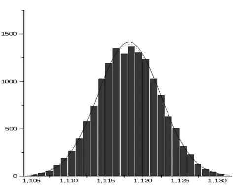
Figure 1 - Distribution of the occurrence frequency for the density of air in a simulation with 15,000 iterations, with temperature of (20.0±1.0)°C, pressure (94,500±6)Pa and humidity (50±5)% (with coverage factor k=1).
Figure 2 - Evaluation of the Number of Iterations: Values of density of air and uncertainty as a function of logarithm of the number of iterations.
14 16 18 20 22 24 26 1,09
1,10 1,11 1,12 1,13
1,14 GUM
MC
D
e
n
s
ity
o
f
a
ir
(
kg
/m
3 )
T (oC)
Knowing the air density distribution (gaussian), it is clear that the uncertainty can be obtained from the standard deviation (or a multiple for an
expanded uncertainty with an associated
confidence level). In what follows, all the results, including those of the input quantities, will be
presented with coverage factor k=1.
One of the main points for using the method of MC is the determination of the number of iterations necessary to obtain a reliable result. A preliminary study was undertaken with the intention to determine the adequate number of iterations. A series of simulations varying the number of iterations were also undertaken , with
temperature ((20.0±1.0)°C), pressure
((94,500±6)Pa) and humidity ((50±5)%) fixed, and
the results are shown in the graph below:
In Fig. 2 one can observe that, about 10,000 iterations (value 4 in axis X), either the density or the uncertainty present a convergence in their
values. Aiming at getting a result with good statistics, it was established that the subsequent would be performed with 70,000 iterations.
Once the number of iterations was established, and the distribution of the density of air was known, several simulations were undertaken. The results
were compared to those obtained with
recommendations of GUM (2003), which can be verified in the next section.
Gum X Monte Carlo
In order to compare both methods two series of results were realized. In the first series the pressure
and humidity were fixed, (94,500±6)Pa and
(50±5)% respectively, while the temperature
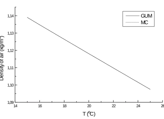
ranged from 15°C to 25°C, with its uncertainty fixed in 1°C in this range. The results of the first series are presented in the following graph:
14 16 18 20 22 24 26 0,0037
0,0038 0,0039 0,0040 0,0041 0,0042
GUM MC
U
n
ce
rt
a
in
ty
D
e
n
s
it
y
(k
g
/m
3 )
T (oC)
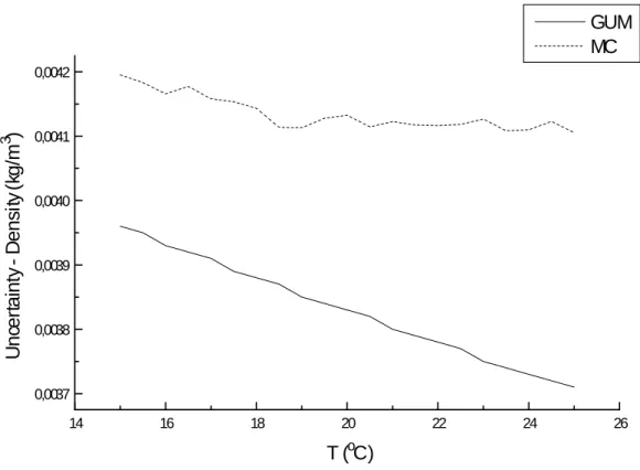
Figure 4 - Values of the uncertainty of the density of air obtained by Monte Carlo and by the recommendations of GUM in the range of temperature from 15°C to 25°C. The solid line represents the results obtained by GUM, while the dot line represents the results of MC.
In Fig. 3 it is clear that both methods, MC and GUM, give identical values of density of air in the range of temperature considered, showing that the density of air decreases as the temperature increases. This seems to be a very obvious result, but it shows explicitly the consistency between both methods (if these curves were not superposed, it would show that the method of Monte Carlo does not converge to the mean value of density, what would make questionable its validity).
The same cannot be said about the uncertainties. As one can see in Fig. 4, the uncertainty obtained by the method of MC has a little decrease and then becomes almost constant with values oscilating
around 0.0041kg/m3, while the uncertainty
obtained by GUM decreases as the temperature
raises along all the range (a decreasing
approximately linear), varying from 0.0040kg/m3
at 15°C to 0.0037kg/m3 at 25°C. It can also be
observed that the uncertainties obtained by GUM (2003) are approximately 5% to 11% smaller than those obtained by MC.
In the second series of results, the temperature and
the humidity were fixed, (20.0±1.0)°C and
(50±5)% respectively, while the pressure were
Figure 5 - Values of the density of air obtained by Monte Carlo and by the recommendations of GUM in the range of pressure from 89,000 Pa to 104,000 Pa. The solid line represents the results obtained by GUM, while the dot line represents the results of MC.
Figure 6 - Values of the uncertainty of the density of air obtained by Monte Carlo and by the recommendations of GUM in the range of pressure from 89,000Pa to 104,000 Pa. The solid line represents the results obtained by GUM, while the dot line represents the results of MC.
88000 90000 92000 94000 96000 98000 100000 102000 104000 106000 1,05
1,10 1,15 1,20 1,25
GUM MC
D
e
n
s
ity
o
f A
ir
(k
g
/m
3 )
P (Pa)
88000 90000 92000 94000 96000 98000 100000 102000 104000 106000 0,0036
0,0038 0,0040 0,0042 0,0044 0,0046
GUM MC
U
n
ce
rt
a
in
ty
D
e
n
s
ity
(k
g
/m
3 )
As before the superposition of the curves in Fig. 5 just shows the consistency of the results obtained by both methods. Regarding uncertainties, one can observe in Fig. 6 that both results increase with the raising of pressure. However, once again one can state that the uncertainties evaluated by GUM
(which varies from 0.0036kg/m3 to 0.0042kg/m3)
are systematically smaller than those obtained MC
(which varies from 0.0039kg/m3 to 0.0045kg/m3).
One can verify that, in this range of pressure under consideration, the uncertainty obtained by GUM is about 10% smaller than that obtained by Monte Carlo. From these results obtained in the two series of simulations, it is clear that the simplest evaluation of uncertainty obtained by the recommendations of GUM (law of propagation of uncertainty for independent quatities) underestimate
the values of uρ, when they are compared with those
obtained Monte Carlo simulations.
FINAL REMARKS
As it can be verified in this study, considering the specific problem of evaluation of uncertainty of the density of moist air by two distincts methods (GUM and MC) and taking into account identical distributions for all input quantities in both
methods, the evaluation of uncertainty via law of
propagation presented values systematically
smaller than those obtained by Monte Carlo simulations, at least in the ranges of temperature and pressure .
These differences can be an indication that, in order to use the law of propagation of uncertainties for the density of moist air, one must consider other terms involving correlation coefficients and/or higher order terms in the Taylor expansion. This case is presently under study by the authors and this is hard task, given the complexity of the expression (2.2.1).
Since the results obtained by the method of MC show no restrictions regarding the behaviour of the output function, the values of uncertainty obtained here seem to be reliable. Therefore, the results obtained by MC could be used to validate a new
evaluation of uncertainty via law of propagation
with higher order terms.
However, when using the simulations of MC, one must be careful because this method, like any other method to evaluate uncertainty, also has its limitations and restrictions, and its use must as
well be very judicious. As such , it is expected that the Supplement to GUM that is in process of elaboration is clear regarding the advantages and limitations of the method.
ACKNOWLEDGEMENTS
The authors would like to thank the staff at CTA for incentive and support.
RESUMO
Neste trabalho são comparados dois métodos de avaliação de incertezas, quais sejam a lei de propagação de incertezas (recomendações do GUM) e o método de Monte Carlo. Como estudo de caso foi utilizada a determinação da densidade do ar úmido. Os resultados mostram que há diferenças entre os dois métodos.
REFERENCES
Canaves Jr., M. and Pompéia, P. J. (2004), Influência da densidade atmosférica na incerteza de medição de massas padrão. [S.l.: s. n.].
Giacomo, P. (1996), Equation for the determination of the density of moist air. Metrologia,18, 33-40. GUM (2003), Guia para a expressão da incerteza de
medição. 3. ed. [S.l.]: INMETRO.
INMETRO (2003), Vocabulário internacional de termos fundamentais e gerais de metrologia - VIM. Portaria Inmetro 029 de 1995. 3. ed. [S.l.]: INMETRO.
Moscati, G.; Mezzalira, L. G. and Santos, F. D. (2004), Incerteza de medição pelo método de Monte Carlo no contexto do “Suplemento 1” do GUM.
Reis, M. L. C. C.; Vieira, W. J.; Barbosa, I.; Mello, O. A. F. and Santos, L. A. (2004), Validation of an external six-component wind tunnel balance calibration. In: Aerodynamic Measurement Technology and Ground Testing Conference, 24., AIAA. Proceedings… AIAA.
Reis, M. L. C.; Lima, D. S. A.; Alvim, R. S. and Camargo, J. B. E. (2004), Avaliação de incerteza em calibração de transdutores de força. [S.l.: s. n.]. Vuolo, J. H. [19--], Fundamentos da teoria de erros.
2. ed. [S.l.]: Edgard Blücher.