1
UNIVERSIDADE DO ALGARVE UNIVERSITY OF ALGARVE
FACULDADE DE CIÊNCIAS E TECNOLOGIA FACULTY OF SCIENCES AND TECHNOLOGY
Towards a Hydrodynamic Operational model of the Algarve Coast and St. Vincent Cape.
ERASMUS MUNDUS EUROPEAN JOINT MASTER IN WATER AND COASTAL MANAGEMENT
MESTRADO EM GESTÃO DA ÁGUA E DA COSTA (CURSO EUROPEU)
SURUJ RAKESH BABWAH
i NOME / NAME:
SURUJ RAKESH BABWAH
DEPARTAMENTO / DEPARTMENT: – Química, Bioquímica e Farmácia
Faculdade de Ciências e Tecnologia (FCT) Universidade do Algarve, Portugal
ORIENTADOR / SUPERVISOR: Flávio Martins,
AREA DEPARTAMENTAL DE ENGENHARIA MECÁNICA UNIVERSIDADE DO ALGARVE, PORTUGAL
DATA / DATE: 22nd February 2011
TÍTULO DA TESE / TITLE OF THESIS:
Hydrodynamic Operational model of the Algarve Coast and St. Vincent Cape.
ii
ACKNOWLEDGEMENTS
I would like to convey my deepest and most heartfelt gratitude to the following persons for their assistance and guidance throughout my thesis and also my European experience.
To my supervisor, Dr. Flávio Martins and my unofficial co-supervisor João Janeiro, for their guidance throughout the course of this thesis. To my course coordinator Professor Alice Newton for her continued support regarding all aspects of my European experience, her continued guidance is priceless. To the European Union for sponsoring this master’s study through the Erasmus Mundus External Co-operation Window Lot 10
Scholarship Programme. To Professor Bheshram Ramlal and Professor Micaheal
Sutherland for their support in the preliminary stages after having accepted the scholarship and for guidance throughout my undergraduate studies. To the many others who have assisted me throughout the course of this body of work and those who continue to do so.
To my immediate family and friends for their continued support and assistance, who have always been there despite the thousands of miles between us, the least I can do is say thank you. And, to my friends, newly found family members who I have met on this amazing journey. With whom I have shared many wonderful and amazing experiences. Thank you (Akilah , Angelika , Baravi , Ndui, Sergei, Shine, Solomon (missing but not forgotten) , Stazi , Teferi , Tina, and Vera ) all for opening your lives to me, thank you all for sharing you culture and your experiences with me.
iii
RESUMO
Este estudo pretende implementar um modelo hidrodinâmico operacionais que podem vir a ser utilizada para projetar padrões de dispersão de vazamento de óleo e também a poluição de esgotos, e pode também ser utilizado na previsão das ondas. Um modelo de duas camadas aninhadas foi criado usando MOHID Água, que é oceano poderoso software de modelagem.
A primeira camada (pai) é usado para impor as condições de contorno para a segunda camada (filho). Isso se repetiu por dois diferentes regimes de ventos dominantes, Easterly e ventos Westerly, respectivamente.
Uma comparação qualitativa foi feita entre os dados medidos de maré e do modelo previsto dados de maré. A temperatura de superfície também foi comparada de forma qualitativa os resultados do modelo. Os resultados de ambas as simulações foram analisados e comparados com a literatura histórica. A comparação foi feita na camada superficial, profundidade de 100 metros e 800m de profundidade. Na camada superficial a primeira simulação gerado um evento de ressurgência, perto do Cabo de São Vicente e no Algarve. A segunda simulação gerado um evento não ressurgência no qual o fluxo superficial foi revertida e que a massa de água quente foi ao longo da costa algarvia e no sentido horário à noite girando em torno do Cabo de São Vicente.
Na profundidade de 100 metros para ambas as simulações, os vórtices de velocidade foram observadas perto do Cabo de São Vicente de viagem norte e sul em várias instâncias.
Em profundidade 800metre um forte fluxo oceânico foi observada em direção ao norte oeste ao longo da plataforma continental.
iv
ABSTRACT
This study attempts to implement a hydrodynamic operational model which can ultimately be used for projecting oil spill dispersal patterns and also sewage, pollution and can also be used in wave forecasting. A two layer nested model was created using MOHID Water, which is powerful ocean modelling software. The first layer (father) is used to impose the boundary conditions for the second layer (son). This was repeated for two different wind dominant regimes, Easterly and Westerly winds respectively. A qualitative comparison was done between measured tidal data and the tidal output. Sea surface temperature was also qualitatively compared with the model’s results. The results from both simulations were analysed and compared to historical literature. The comparison was done at the surface layer, 100 metre depth and at 800m depth. In the surface layer the first simulation generated an upwelling event near Cape St. Vincent and within the Algarve. The second simulation generated a non-upwelling event within which the surface was flow reversed and the warm water mass was along the Algarve coastline and evening turning clockwise around Cape St. Vincent.
At the 100 metre depth for both simulations, velocity vortexes were observed near Cape St. Vincent travelling northerly and southerly at various instances.
At 800metre depth a strong oceanic flow was observed moving north westerly along the continental shelf.
Keywords : forecasting , operational model, MOHID, nested, simulation
v Contents
ACKNOWLEDGEMENTS ... ii
RESUMO ... iii
ABSTRACT ... iv
LIST OF FIGURES ... viii
LIST OF EQUATIONS ... xi
LIST OF TABLES ... xii
Chapter 1 ... 1
1.1 Introduction ... 1
1.2 :Project Justification ... 1
1.3 :Operational Models. ... 2
1.3.1 . :State of the art ... 2
1.4.1 :MOTHY MODEL ... 3
1.5.1 :Storm surge prediction in Venice ... 4
Chapter 2 Mohid Modelling ... 6
2.1 :Overview ... 6
2.1.1 . :History ... 6
2.1.3 . :Mohid Program Design ... 7
2.2 MOHID Modules ... 10
2.2.3 . Hydrodynamic Module ... 12
vi
2.2.4.1. Temporal discretization ... 17
2.2.5 Boundary Conditions ... 17
2.2.5.1 Free surface ... 17
2.2.5.2 Bottom boundary ... 18
2.2.5.3 Lateral closed boundaries ... 19
2.2.5.4 Open boundaries ... 20
2.2.5.5 Moving boundaries ... 21
2.2.4 Water Properties Module ... 22
2.2.5 Lagrangean Module ... 24
2.3 Data Assimilation ... 26
2.3.1 Continuous Assimilation ... 27
2.4 Applications ... 29
CHAPTER 3 : SITE DESCRIPTION ... 31
3.1 Iberia ... 31
3.2 Algarve ... 35
3.2.3 Tidal Regime ... 38
3.2.4 Upwelling ... 38
3.3 Cape St. Vincent ... 41
CHAPTER 4: Simulation Implementation ... 44
4.1 . Data Description ... 44
4.1 .1Bathymetry ... 44
vii
4.1.0.3. Wind ... 45
4.2 . Method (Structure of the model and boundary conditions) ... 45
CHAPTER 5 : RESULTS ... 48
5.1 . JUNE ... 48
JULY ... 52
CHAPTER 6: Discussion and Conclusions ... 60
6.1 Tides ... 60 6.2 Surface layer ... 60 6.3 100m Depth ... 62 6.4 800m Depth ... 64 6.5 Satellite Imagery ... 65 6.6 Conclusion ... 66 CHAPTER 7 : Bibliography ... 68 Appendice 1 ... 73 Appendix 2 ... 75 Appendix 3 ... 77
viii
LIST OF FIGURES
Figure 1 Illustrative grid showing the potentialities of the vertical discretization of the
MOHID system adapted from Martins(1999) ... 16
Figure 2: Volume element used in the discretization. Adapted from Martins (1999). ... 17
Figure 3: Random movement caused by an eddy larger than the particle ... 25
Figure 4: Random movement forced by an eddy smaller than the particle ... 26
Figure 5: Geography of the Western Iberian system, showing the main features referred to in the text. The 200 m bathymetric contour, that roughly delimits the continental shelf, is represented. From north to south: CO, Cape Ortegal; CF, Cape Finisterre; OC, Oporto Canyon; AC, Aveiro Canyon; NC, Nazare´ Canyon; CC, Cape Carvoeiro; CR, Cape Roca; CE, Cape Espichel; SB, Setu´bal Bay; CS, Cape Sines; CSV, Cape Sa˜o Vicente; PC, Portima˜o Canyon; CSM, Cape Santa Maria.(Relvas et al. 2007) ... 32
Figure 6: Showing the study area. (source: Google Earth 2010) ... 35
Figure 7 Surface Circulation on The Eastern North Atlantic (Martins et al. 2002) ... 37
Figure 8 : Showing coastal upwelling along the Sagres coastline SW-Portugal ... 40
Figure 9: Graph Comparing Predicted tidal data against Measured tidal data from Lagos station. ... 48
Figure 10 :Hydrodynamics of the Algarve plotted upon the water temperature. ... 49
Figure 11: Depth of appromiately 25m ... 50
Figure 12: approximately 100m depth ... 50
Figure 13: approximately 100m depth ... 51
Figure 14 :800 m ... 52
Figure 15: Tidal data comparison between mohid predicted tide and tide gauge data from Lagos. ... 52
ix
Figure 17: 25m depth ... 54
Figure 18: Depth of 100m ... 54
Figure 19:Depth 100m ... 55
Figure 20: Depth of 800m ... 55
Figure 21: Satellite Image obtained from My Ocean showing sea surface temperature for Portugal, Spain and Morocco. ... 57
Figure 22: Showing extracted portion from previous image. ... 58
Figure 23: Image showing forecasted sea surface temperature. ... 58
Figure 24: Showing the daily average wind speed and Direction for the June simulation period. ... 59
Figure 25: Showing the daily average wind speed and direction for the July simulation period. ... 59 Figure 26 ... 73 Figure 27 ... 73 Figure 28 ... 74 Figure 29 ... 74 Figure 30 ... 75 Figure 31 ... 75 Figure 32 ... 76 Figure 33 ... 76 Figure 34 ... 77 Figure 35 ... 77 Figure 36 ... 78 Figure 37 ... 78 Figure 38 ... 79
x
xi
LIST OF EQUATIONS
Equation 1 ... 12 Equation 2 ... 12 Equation 3 ... 13 Equation 4 ... 13 Equation 5 ... 13 Equation 6 ... 13 Equation 7 ... 13 Equation 8 ... 14 Equation 9 ... 15 Equation 10 ... 15 Equation 11 ... 18 Equation 12 ... 18 Equation 13 ... 18 Equation 14 ... 18 Equation 15 ... 19 Equation 16 ... 19 Equation 17 ... 19 Equation 18 ... 20 Equation 19 ... 20 Equation 20 ... 20 Equation 21 ... 21 Equation 22 ... 22 Equation 23 ... 22 Equation 24 ... 22xii Equation 25 ... 23 Equation 26 ... 25 Equation 27 ... 28 Equation 28 ... 39
LIST OF TABLES
Table 1: The three main programs n MOHID system and their generic use(Braunschweig et al.). ... 8Table 2:Different “Class” levels of MOHID (Braunschweig et al.). ... 9 Table 3: List of the main modules used in MOHID. Reproduced from (Neves 2003) 10
1
Chapter 1
1.1 Introduction
The increase of human occupation in the world coastlines makes disasters that much more devastating than in last 50 years. Many countries depend heavily upon coastal tourism, so any type of coastal disaster, natural or manmade affects the lively hood of many more people than in previous years. Also fisheries are prone to any sort of toxic spill, most notably oil spills.
Initial objectives:
To set up a pre-operational system of nested models which simulate the hydrodynamics of the Algarve Coast and St. Vincent Cape.
• Implement a set of Grids and bathymetry for the region.
• Identify operational data available and integrate it as boundary conditions for this system.
• Run model simulations for calibration purposes. • Identify available data for model calibration.
1.2 :Project Justification
As a coastal manager it is necessary to understand the hydrodynamics that occurs within the coastal zone. Knowledge of this nature is vital in understanding pollution dispersal and the general dynamics of the location.
Hence, modelling is a vital part of this equation. Nowadays, modelling is commonly used both as a forecasting and as an investigative tool aiding the decision making process.
The modelling tool that will be developed in this thesis can also be used to implement an early warning system to predict, prevent and mitigate future problems.
2
1.3 :Operational Models.
1.3.1 . :State of the art
Within recent years, the importance of operational oceanography and data assimilation systems has been growing. There are many different systems and these all use varied types of data streams and have varied specific purposes. In general, they all aim to support a range of scientific and operational applications including oil spill monitoring, marine safety, and wave forecasting (Daniel P, 2005). Several European operational oceanography and data assimilation systems have been implemented in the last few years. Some examples are the POSEIDON system (Nittis et al. 2001) generally used for oil spills, the MOTHY model (Daniel P, 2005) created for predicting the drift of pollutants and the SHYFEM model (Bajo et al. 2007) utilized for storm surge prediction in Venice.
The POSEIDON system is based on OCEANOR's Sea-watch system, it was developed and operated by the Hellenic Centre for Marine Research (HCMR)(Hansen et al. 1997). The POSEIDON framework consists of a network comprised of 10 oceanic and 10 wave bouys deployed throughout Greece. These are all equipped with sensors necessary for monitoring the offshore environment.
Properties like wind speed and direction, air pressure and temperature, surface water temperature, sea-surface current speed and direction, wave height and direction, water temperature and salinity, dissolved oxygen, chlorophyll-a and nitrates are measured, quality controlled, stored and pre-processed in an automated way through a computing system and software present in all sensors and are near real-time remotely transmitted to
3 the Operational Centre of HCMR by a two-way telecommunication (http://poseidon.hcmr.gr/listview.php?id=5).
The POSEIDON system is comprised of separate but yet interrelated fractions. HCMR’s Operational Centre controls and handles the surveillance of the system. The POSEIDON’s forecasting ability comes from the Aegean Operational Forecasting System (AOFOS). This system is tailored to suit the Greek sea environment by means of numerical simulations and forecast models. A more detailed description is given in Nittis et al. (2001).The systems skeletal structure is comprised of a weather prediction model, an open sea wave forecast model, a 3D hydrodynamic model, a shallow water wave prediction model and a buoyant pollutant transport model.
The POSEIDON OSM (Oil Spill Model) can be used either in forecasting mode or hindcasting mode. The user is also allowed to input oil spill scenarios providing all the necessary parameters. The final output consists of a series of sequential graphs showing the oil spill dispersion for the requested time period (Soukissina et al. 2000).
1.4.1 :MOTHY MODEL
“The MOTHY model developed by Météo-France is used on an operational basis to predict the drift of pollutants on the ocean surface” (Daniel et al. 2005) .It is based on a hierarchy of nested limited domain ocean models coupled to a pollutant dispersion model. The model is also forced by wind and pressure fields provided atmospheric models. These atmospheric models can be the IFS model (European Centre for Medium Range Weather Forecasts) or the ARPEGE model (Courtier et al. 1991).
This system was specifically created to forecast drift. Currents are computed in such a way so as to represent vertical current shear. This was done by following the work of
4 Poon et al. (1991) a shallow water model coupled with a turbulent viscosity model with a bilinear eddy viscosity profile was utilized.
This approach is well suited for large areas if the major currents in the study area are considered negligible (Daniel 2005) .However if these currents have a profound impact on the dynamics of the study area, a forecaster is needed to review the forecasted data. The oil slick itself is modelled in such a way that it considers the oil droplets to be independent and their movement is influenced by its own buoyancy and oceanic parameters such as currents and turbulence. In general 90%-95% of oil droplets remain on the surface. This is because the buoyancy is dependant upon the size and density of the oil droplets, thus larger droplets stay on the surface and the smaller ones are mixed in the upper surface layer of the water column (Comerma et al. 2002).The model calibration is documented in Daniel (1996). It was based upon several pollution incidents.
1.5.1 :Storm surge prediction in Venice
Although not intended for the management of the flood barriers, forecasting water levels is also important to alert businesses, warehouses and tourist-related activities of flooding events. The SHYFEM model was previously used operationally for numerically predicting storm surges in the northern Adriatic Sea.
5
1.5.2 :Numerical model
The Core of the forecasting system is the SHYFEM Model. It is an open source project developed at CNR-ISMAR in Venice. The code is freely downloadable from the web page: http://www.ve.ismar.cnr.it/shyfem and can be compiled under a variety of Unix and Linux like operating systems. The Shallow-water Hydrodynamic Finite Element Model (SHYFEM), developed at ISMAR-NR of Venice (Bajo et al. 2007) is operational at ICPSM since November 2002 (Canestrelli et al. 2005).
1.5.3 :Meteorological data
The European Centre for Medium-Range Weather Forecasts (ECMWF) provides the wind and atmospheric data used by the model. The Centro Nazionale di Meteorologia e Climatologia Aeronautica (CNMCA, the Aeronautic National Centre of Meteorology and Climatology of the Italian Air Force) distributes in real time the analysis and forecast fields. The centre supplies mean sea level pressure and surface wind fields over the Mediterranean area. On a daily basis a server from the CNMCA in Rome, transfers the meteorological fields to a dedicated server at the ICPSM (Bajo et al. 2007).
1.5.4 :The operational procedure
On a daily basis the procedure begins with a connection to a storage server of the ICPSM centre, upon which a complete data set for meteorological forcing is downloaded. Upon completion of this task, the data is then spatially interpolated to the finite element grid of the Mediterranean Sea.The forcing data is applied and simulation commences. The simulated data produces hourly forecasts with a range of up to 6 days in advance. At the end of the simulation, model results are summed to the computed astronomical tide and a prediction of the total sea level is provided (Bajo et al. 2007).
6
Chapter 2 Mohid Modelling
2.1 :Overview
This chapter describes the three-dimensional (3D) water modelling system MOHID and provides an insight on the modules used in this work. The MOHID model is being developed by a large team from the Instituto Superior Técnico (IST), Portugal, in close cooperation with Hidromod Lda and includes contributions from the permanent research team and from a large number of PhD students on Environmental and Mechanical Engineering from IST master course on Modelling of the Marine Environment. Contributions from other research groups have also been very important for the development of the model (Neves et al. 2003).
2.1.1 . :History
The first version of the MOHID modelling software was created in 1985. With the passing of time, the software matured with continuous updates and improvements to its use in the framework of many research and engineering projects. MOHID was initially a bi-dimensional tidal model (Neves 1985).
As part of the MOHID system other models were created, bi-dimensional euleran and lagrangian transport modules were also included with a Boussinesq model for non-hydrostatic gravity waves (Silva 1992).
Santos (1995) introduced the first three dimensional model. This model utilized a double sigma coordinate system (MOHID 3D). However, the double sigma coordinate system had many limitations. This impressed the need for a model which could use a generic vertical coordinate, allowing the user to have a choice among several coordinates, depending on the main processes in the study area (Neves 2003).
Martins (1999) answered the call for this necessity by introducing the version Mesh 3D with a generic vertical coordinate and formulated infinite volumes. In the Mesh 3D
7 model, a 3D eulerian transport model, a 3D lagrangian transport model and a zero-dimensional water quality model were included. This version of the model revealed that the use of an integrated model based on a generic vertical coordinate is a very powerful tool. However, due to the extended limitations of the FORTRAN 77 language the model was difficult to maintain. A decision was then made to reorganise the model in an object oriented architecture, using FORTRAN 95 potentialities (Neves 2003).
2.1.3 . :Mohid Program Design
Initially MOHID was a bi-dimensional tidal model developed by Neves, (1985) who applied the model in the study of estuaries and coastal areas using a classical finite-difference approach. In 1998 the whole code was submitted to a complete rearrangement with the main objective of producing a more robust and reliable model and to protect its structure against involuntary programming errors. To achieve this goal, object oriented programming using FORTRAN 95 was introduced in the MOHID model. Some of the techniques used are described in Decyk et al. (1997). The new philosophy of the model (Miranda et al. 2000) permits the use of the model in any dimension (one-dimensional, two-dimensional or three-dimensional). The whole model is programmed in ANSI FORTRAN 95, using the objected orientated philosophy.
8 The model was restructured and converted to ANSI FORTRAN 95, profiting from its new features such as the ability to use object oriented programming methods. Source code written according to the F95 standards assures that MOHID Framework applications can run in any operative system that supports a F95 compiler (Leitão 2003).
This migration began in 1998, implementing object oriented features as described by Decyk et al. (1997) with significant changes in code organisation (Miranda et al. 2000) This ultimately led to an object oriented model for surface water bodies which integrates different scales and processes The modular architecture from object-oriented model was the basis for the creation of the current which is a system of several numerical tools There are three main programs: (i) MOHID Water, (ii) MOHID Land and (iii) MOHID Soil.
Table 1: The three main programs n MOHID system and their generic use(Braunschweig et al.).
MOHID Water It is an updated version to simulate processes in free surface water bodies .
MOHID Land It is used to model river basins
MOHID Soil Intended to study processes in ground water porous media(saturated and unsaturated).
Nowadays, Mohid Water Modeling System is robust and reliable system for modelling and integrated water resources management.
The FORTRAN 95 is not primarily an object-oriented language, but can be used for object-oriented programming. The modules generated in FORTRAN can be used as classes(Decyk et al. 1997; Akin et al. 2002).
The architecture of MOHID is based on different programming features. The classes that form the MOHID Framework were designed on a common basis, regarding programming rules and definition concepts in order to establish a straightforward
9 connection of the whole code. “This is reflected in memory organization, public
methods systematisation, possible object states, client/server relations and errors management” (Leitão 2003).
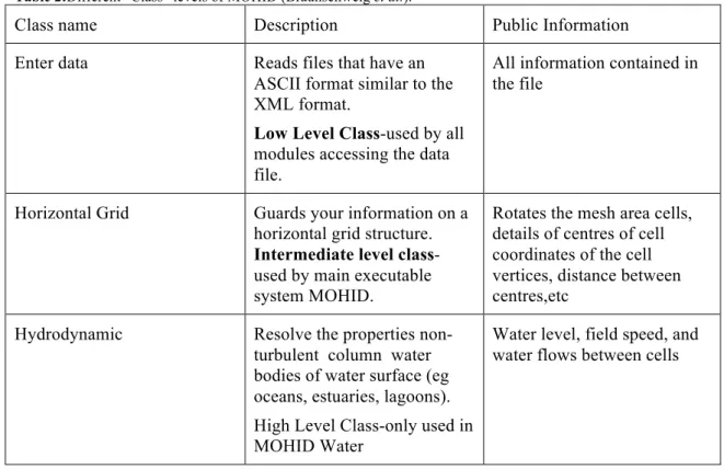
whole model structure is divided into modules, which each respective module to feature a certain class. The table below lists and describes three such examples of different class levels.
Table 2:Different “Class” levels of MOHID (Braunschweig et al.).
Class name Description Public Information Enter data Reads files that have an
ASCII format similar to the XML format.
Low Level Class-used by all
modules accessing the data file.
All information contained in the file
Horizontal Grid Guards your information on a horizontal grid structure.
Intermediate level class-
used by main executable system MOHID.
Rotates the mesh area cells, details of centres of cell coordinates of the cell vertices, distance between centres,etc
Hydrodynamic Resolve the properties non-turbulent column water bodies of water surface (eg oceans, estuaries, lagoons). High Level Class-only used in MOHID Water
Water level, field speed, and water flows between cells
The whole model is programmed in ANSI FORTRAN 95, using the objected orientated philosophy. The subdivision of the program into modules, like the information flux between these modules was object of a study by the Mohid authors.
10
2.2 MOHID Modules
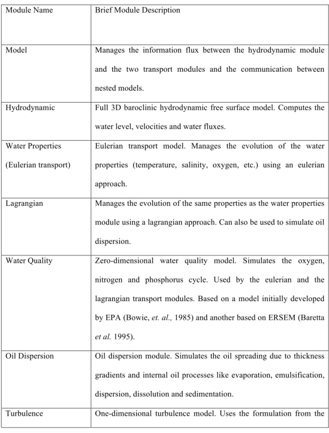
MOHID is composed by over 40 modules which complete over 150 mil code lines. Each module is responsible to manage a certain kind of information. The main modules are the modules listed in the following table.
Table 3: List of the main modules used in MOHID. Reproduced from (Neves 2003) Module Name Brief Module Description
Model Manages the information flux between the hydrodynamic module and the two transport modules and the communication between nested models.
Hydrodynamic Full 3D baroclinic hydrodynamic free surface model. Computes the water level, velocities and water fluxes.
Water Properties (Eulerian transport)
Eulerian transport model. Manages the evolution of the water properties (temperature, salinity, oxygen, etc.) using an eulerian approach.
Lagrangian Manages the evolution of the same properties as the water properties module using a lagrangian approach. Can also be used to simulate oil dispersion.
Water Quality Zero-dimensional water quality model. Simulates the oxygen, nitrogen and phosphorus cycle. Used by the eulerian and the lagrangian transport modules. Based on a model initially developed by EPA (Bowie, et. al., 1985) and another based on ERSEM (Baretta
et al. 1995).
Oil Dispersion Oil dispersion module. Simulates the oil spreading due to thickness gradients and internal oil processes like evaporation, emulsification, dispersion, dissolution and sedimentation.
11 GOTM model.
Geometry Stores and updates the information about the finite volumes.
Boundary Conditions Surface-Boundary conditions at the top of the water column. Bottom-Boundary conditions at the bottom of the water column. Open-Boundary conditions at the frontier with the open sea.
Discharges River or Anthropogenic Water Discharges
12
2.2.3 . Hydrodynamic Module
The hydrodynamic module solves the three-dimensional incompressible primitive equations. Hydrostatic equilibrium and Boussinesq approximation is assumed. The momentum balance equations for mean horizontal flow velocities are, in Cartesian form:
( )
uu( )
uv( )
uw u x y z t =−∂ −∂ −∂ ∂(
)
(
v v u)
(
(
v v)
u)
(
(
v v)
u)
p fv− ∂x +∂x H + ∂x +∂y H + ∂y +∂z t + ∂z + 0 1 ρ Equation 1( )
vu( )
vv( )
vw v x y z t =−∂ −∂ −∂ ∂(
)
(
v v v)
(
(
v v)
v)
(
(
v v)
v)
p fu− ∂y +∂z H + ∂x +∂y H + ∂y +∂z t + ∂z − 0 1 ρ Equation 2Where u, v and w are the Reynolds averaged components of the velocity vector in the x, y and z directions respectively, f the Coriolis parameter, νH and νt the turbulent
viscosities in the horizontal and vertical directions, ν is the molecular kinematic viscosity (equal to 1.3x10⁻⁶ m2 s-1) and p is the pressure. The temporal evolution of
velocities (term on the left hand side) is the balance of advective transports (the first three terms on the right hand side), Coriolis force (forth term), pressure gradient (fifth term) and turbulent diffusion (last three terms).
13 The vertical velocity is calculated from the incompressible continuity equation (mass balance equation): 0 = ∂ + ∂ + ∂xu yv zw Equation 3
by integrating between bottom and the depth z where w is to be calculated:
( )
∫
∫
− − ∂ − −∂ = z h z h y x udz vdz z w Equation 4The free surface equation is obtained by integrating the equation of continuity over the whole water column (between the free surface elevation η(x,y) and the bottom -h):
∫
∫
− − ∂ − −∂ = ∂ η η η h h y x t udz vdz Equation 5The hydrostatic approximation is assumed which reduces the vertical momentum equation to: 0 = + ∂zp g
ρ
Equation 6where g is gravity and ρ is density. If the atmospheric pressure patm is subtracted from p,
and density ρ is divided into a constant reference density ρ0 and a deviation ρ' from that
constant reference density, after integrating from the free surface to the depth z where pressure is calculated :
( )
z p g(
z)
g dz p z atm+ − +∫
ʹ′ = η ρ η ρ0 Equation 714 This relates pressure at any depth with the atmospheric pressure at the sea surface, the sea level and the pressure anomaly integrated between that level and the surface. By using this expression and the Boussinesq approximation, the horizontal pressure gradient in the direction xi can be divided in three contributions:
∫
ʹ′ ∂ − ∂ − ∂ = ∂ η ρ η ρ z x x atm x xip ip g 0 i g i dz Equation 8The total pressure gradient is the sum of the gradients of atmospheric pressure, of sea surface elevation (barotropic pressure gradient) and of the density distribution (baroclinic pressure gradient).
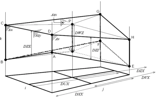
15 2.2.4 SPATIAL DISCRETIZATION
The model uses a finite volume approach (Chippada et al. 1998; Martins et al. 2001) to discretize the equations.
In this approach, the discrete form of the governing equations is applied macroscopically to a cell control volume. A general conservation law for a scalar U, with sources Q in a control volume Ω is written as:
∫
∫
∫
Ω Ω Ω = + Ω ∂ S t Ud FdS Qd Equation 9Where F are the fluxes of the scalar through the surface S embedding the volume. After discretizing this expression in a cell control volume j where U is defined, we obtain:
(
)
j j faces j j tU Ω + F⋅S =Q Ω ∂∑
Equation 10In this form, the solution for the equations is independent of cell geometry. The cell is able to take on any shape with very few constraints (Martins 1999) since only fluxes among the cell faces are required. Geometry is achieved from this because of the complete separation of the physical variables (Hirsch 1988).
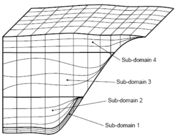
The geometry is continuously updated in every time step because volumes can vary in their course of the calculus. The spatial coordinates are, independent: this means that any vertical geometry can be chosen for the mesh. Cartesian or curvilinear coordinates can be used in the horizontal and a generic vertical coordinate with different sub
16 domains can be used in the vertical direction (Janeiro 2006) (Figure below). This general vertical coordinate allows minimizing the errors of some of the classical vertical coordinates (Cartesian, sigma, isopycnical) as pointed in Martins et al(2001).
.
Figure 1 Illustrative grid showing the potentialities of the vertical discretization of the MOHID system adapted from Martins(1999)
Only a vertical degree of freedom is allowed, and the grid is Cartesian orthogonal in the horizontal. The grid is staggered in the horizontal in an Arakawa C manner, i.e. horizontal velocities are located in the centre of the west (u-velocity) and south (v-velocities) faces, while elevation, turbulent magnitudes and tracers are placed in the centre (Martins 1999).
Also a staggering in the vertical is used, with vertical velocity w, vertically placed in the top and bottom faces and tracers and turbulent magnitudes in the centre of the element (in vertical) (Martins 1999).
17 Figure 2: Volume element used in the discretization. Adapted from Martins (1999).
2.2.4.1. Temporal discretization
The temporal discretization is carried out by means of a semi implicit ADI (Alternate Direction Implicit) algorithm. This algorithm computes alternated one component of horizontal velocity implicitly while the other is calculated explicitly. The resulting equation system is a tridiagonal one, which can be solved by the Thomas algorithm in an efficient and quick way. This allows preserving the stability advantages of implicit methods without the draw-backs of computational expensiveness and associated phase errors. A longer time-step can therefore be used. A full description of the discretization may be found in Martins (1999).
2.2.5 Boundary Conditions
2.2.5.1 Free surface
All advective fluxes across the surface are assumed to be null. This condition is imposed by assuming that the vertical flux of W at the surface is null:
18 Equation 11
Diffusive flux of momentum is imposed explicitly by means of a wind surface stress
Equation 12
Wind stress is calculated according to a quadratic friction law:
Equation 13
where CD is a drag coefficient that is function of the wind speed, ρa is air density and
is the wind speed at a height of 10 m over the sea surface.
Temperature and salinity advective fluxes are imposed null. Other fluxes of heat and freshwater are introduced as source/sink terms in the transport equations (described in Water Properties Module).
2.2.5.2 Bottom boundary
Also at the bottom, advective fluxes are imposed as null and diffusive flux of momentum is estimated by means of a bottom stress that is calculated by a non-slip method with a quadratic law that depends on the near-bottom velocity. So, the diffusive term at the bottom is written as:
19 CD is the bottom drag coefficient that is calculated with the expression:
Equation 15
Herein is the k the Von Karman-constant and the bottom roughness lenth. Default values are κ = 0.4and = 0.0025 m. The bottom stress term is computed implicitly bin MOHID.
2.2.5.3 Lateral closed boundaries
At these boundaries, the domain is limited by land. For the spatial resolution used here this lateral boundary layer is not resolved, for that reason an impermeable, free slip condition is used:
Equation 16
Equation 17
In the finite volume formalism, these conditions are implemented straightforwardly by specifying zero normal water fluxes and zero momentum diffusive fluxes at the cell faces in contact with land.
20 2.2.5.4 Open boundaries
Open boundaries arise from the necessity of confining the domain to the region of study. The values of the variables must be introduced there such that it is guaranteed that information about what is happening outside the domain will enter the domain in a way that the solution inside the domain is not corrupted. Several different open boundary conditions were already introduced in MOHID (Santos 1995; Martins 1999; Montero 1999).
Two methods of open boundary conditions (OBC) can be used in MOHID : radiative methods and nudging (relaxation) method).
The Dirichelet condition (clamped) can be regarded as the simplest form of active boundary condition where the field, Φ, is connected at the boundary to a reference solution, Φ , ext ext Φ = Φ Equation 18
The concept is generalized with the linear boundary operator B, and a general class of simple active boundary condition follow the relation
ext
ΒΦ = ΒΦ Equation 19
The particular case of the clamped condition considers B = id. When only the external water level is known, then the Blumberg method (Blumberg and Kantha, 1985), consisting of a combination between a nudging term and the Sommerfeld condition, may be used: lag ref T n c t η η η η − − = Δ ⋅ + ∂ ∂ Equation 20
21 Where Tlag is the relaxation decay time. For the other variables, where no accurate
estimation of their celerity is available, another class of OBC method is implemented in MOHID: the relaxation method. It consists on a looser approach to the clamped (Dirichelet) conditions on the open boundary Γ of the domain Ω (Blayo et al. 2005)where a relaxation decay time is introduced and an additional domain is created Ωs, close to the boundary where the condition is applied. This approach is commonly regarded as a Flow Relaxation Scheme (FRS) (Martinsen et al. 1987). The relaxation term writes: lag ref T t Φ − Φ − = ∂ Φ ∂ Equation 21
Where Φ is the relaxed variable, Φref is the reference solution and Tlag is the relaxation
decay time. Additionally, in order to smooth out the nudging at Ωs, a sponge layer, consisting of a high viscosity layer, can also be implemented in MOHID.
2.2.5.5 Moving boundaries
Moving boundaries are closed boundaries that change position in time. If there are intertidal zones in the domain, some points can be alternatively covered or uncovered depending on tidal elevation. A stable algorithm is required for modelling these zones and their effect on hydrodynamics of estuaries. A detailed exposition of the algorithms used in MOHID can be found in Martins(1999).
22 2.2.4 Water Properties Module
The water properties module computes the evolution of the water properties in the water column, using an Eularian approach. This includes the transport due to advective and diffusive fluxes, water discharges from rivers or anthropogenic sources, exchange with the bottom (sediment fluxes) and the surface (heat fluxes and oxygen fluxes), sedimentation of particulate matter and the internal sinks and sources (water quality). The model solves transport equations for salinity and temperature:
Equation 22
Equation 23
With v′h and v′t the horizontal and vertical eddy diffusivities of salt and temperature
(considered to be equal), and v′T and v′s the molecular diffusivities of salt and
temperature (1.1x10⁻⁹ and 1.4x10⁻⁷ m2s-1). The temporal evolution of S and T is the
balance of advective transport by the mean flow, turbulent mixing and the contributions of FT and FS, the possible sinks or sources of temperature and salinity.
The transport due advective and diffusive fluxes, of a given property A, is resolved by the following equation:
23 The density ρ is calculated as a function of temperature and salinity by a simplified equation of state (Leendertsee et al. 1978):
Equation 25
That is an approximation for shallow water of the most widely used UNESCO equation (UNESCO 1981).
At present the MOHID model can simulate 24 different water properties: temperature, salinity, phytoplankton, zooplankton, particulate organic phosphorus, refractory dissolved organic phosphorus, non-refractory dissolved organic phosphorus, inorganic phosphorus, particulate organic nitrogen, refractory organic nitrogen, non-refractory organic nitrogen, ammonia, nitrate, nitrite, biological oxygen demand, oxygen, cohesive sediments, ciliate bacteria, particulate arsenic, dissolved arsenic, larvae and fecal coliforms. In the water quality module, the nitrogen, oxygen and phosphorus cycle can simulate the terms of sink and sources.
24 2.2.5 Lagrangean Module
Lagrangean transport models are very useful to simulate localized processes with sharp gradients (submarine outfalls, sediment erosion due to dredging works, hydrodynamic calibration, oil dispersion, etc.).
MOHIDS’s lagrangean module uses the concept of tracer, which varies according to the application of the model. For a physicist a tracer can be a water mass, for a geologist it can be a sediment particle or a group of sediment particles and for a chemist it can be a molecule or a group of molecules. A biologist can spot phytoplankton cells in a tracer (at the bottom of the food chain) as well as a shark (at the top of the food chain), which means that a model of this kind needs to simulate a wide spectrum of processes (Neves 2003).
The tracers are characterized by their spatial coordinates, volume and a list of properties (each with a given concentration). Each tracer has associated a time to perform the random movement. The tracers are “born” at origins. Tracers which belong to the same origin have the same list of properties and use the same parameters for random walk, decay, etc. Origins can differ in the way they emit tracers. There are three different ways to define origins in space:
• A “Point Origin” emits tracers at a given point; • A “Box Origin” emits tracers over a given area;
• An “Accident Origin” emits tracers in a circular form around a point;
There are two different ways in which origins can emit tracers in time:
• A “Continuous Origin” emits tracers during a period of time; • An “Instantaneous Origin” emits tracers at one instant;
25 Origins can be grouped together in Groups. Origins which belong to the same group are grouped together in the output file, so it is easier to analyze the results (Neves 2003). The most important property of a tracer is its position (x,y,z). The major factor responsible for particle movement is generally the mean velocity. The spatial coordinates are given by the definition of velocity:
Equation 26
where u stands for the mean velocity and x for the particle position. Velocity at any point of space is calculated using a linear interpolation between the points of the hydrodynamic model grid. The Lagrangean module permits to divide the calculation of the trajectory of the tracers into sub-steps of the hydrodynamic time step.
Turbulent transport is responsible for dispersion, the effect of eddies over particles depends on the ratio between eddies and particle size. Eddies bigger than the particles make them move at random as explained below
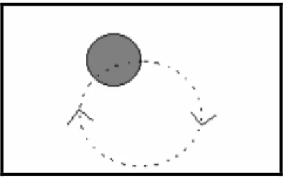
Figure 3: Random movement caused by an eddy larger than the particle
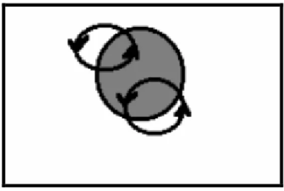
Eddies smaller than the particles cause entrainment of matter into the particle, increasing its volume and its mass according to the environment concentration, seen below.
26 Figure 4: Random movement forced by an eddy smaller than the particle
The random movement is calculated following the procedure of Allen (1982). The random displacement is calculated using the mixing length and the standard deviation of the turbulent velocity component, as given by the turbulence closure scheme of the hydrodynamic model. Particles retain that velocity during the necessary time to perform the random movement, which is dependent on the local turbulent mixing length. The increase in volume is associated with small-scale turbulence and is reasonable to assume it as isotropic. In these conditions, small particles keep their initial shape and increase in volume as a function of its volume. To simulate oil dispersion the Lagrangean module interacts with the oil dispersion module.
2.3 Data Assimilation
“Data assimilation consists of combining the modelled fields with data observed at various points in the domain to produce the best possible estimate of the real state of the ocean over the entire model domain”(Tucker et al. 2004).
Numerical Weather Prediction and Ocean Prediction centres use assimilation techniques. Generally, the data prediction for the present time, is coupled with observed measurements and utilized for the next model forecast. The forecast accuracy depends upon the integrity of the present model state. This occurs because errors propagate
27 throughout the model. Thus, the larger the error in the earlier stages, the less accurate the forecast measurements (Kantha et al. 2000).
2.3.1 Continuous Assimilation
The model is kept continuously operating and data is assimilated as they become available. The fields are continuously updated to produce a nowcast. A similar model running at the same time can then produce a forecast without any data assimilation. A forecast can then be initiated at any point by a similar model running forward free without any data assimilation, but initialized from the sate of the nowcast model. Continuous assimilation has a tendency to reduce the stabilization period in the model system from the assimilation of the data. This factor makes it preferable in most cases. The principle disadvantage is the cost of running the nowcast model, in addition to the forecast model (Kantha et al. 2000).
2.3.2 Direct Insertion
This method is seldom used in meteorology and oceanography because the compounded errors are too great for the precise nature of metrological predictions. This method is utilized for oceanographic data because the tolerance margin for errors is greater. In this method, the model’s predicted values are simply replaced by observed values at key grid points (where observation is available). The basic assumption is that the model data has too many large errors thus the observed data is accurate. A variation of this method is replacing the model generated values at grid intervals with observed data in a continuous assimilation scheme, with each input carrying its own specific weighting factor. It is expected of the model that it will be able to spread the information form observation to more nearby grid points. This method is fairly simple and thus widely utilized (Kantha et al. 2000).
28
2.3.3 Nudgeing
This method is often used in meteorology as well as oceanography. This method actually alters the governing physics and hence must be used with extreme care.
Equation 27
Where the model X is nudged toward a reference value X0 (in this case the observed
value) at a timescale TD. X0 can itself be a function of time. The smaller the value of TD,
the more rapidly it is nudged towards the reference value, since as TD approaches 0 , X
approaches X0 .
2.3.4 Kalman filter
The Kalman filter is very powerful in several aspects. It is a set of mathematical equations used to compute the errors inherent in a system. This filter supports estimations of past, present and future states. The Kalman filter estimates a process by using a form of feedback control: the filter estimates the process state at some time and then obtains feedback in the form of (noisy) measurements. This filter computes the process state at a specific time period and then obtains measurements in the form of feedback (noisy measurements). Because of this, the equations for the Kalman filter fall into two specific categories: time update equations and measurement update equations(Welch et al. 2006).
The time update equations are responsible for present case scenarios and forecasting. It is also responsible for the error covariance estimates used to obtain the a priori estimates for the next time step(Welch et al. 2006).
29 “The measurement update equations are responsible for the feedback”(Welch et al. 2006). This basically means that these equations are responsible for making the necessary corrections to the data. A more detailed explaination of the Kalman filter and the associated formulae can be found in Welch et al. (2006).
2.4 Applications
The MOHID model has been applied to several coastal and estuarine areas and it has showed its ability to simulate complex features of the flows. Several different coastal areas have been modelled with MOHID in the framework of research and consulting projects. Along the Portuguese coast, different environments have been studied, including the main estuaries (Minho, Lima, Douro, Mondego, Tejo, Sado, Mira, Arade and Guadiana) and coastal lagoons (Ria de Aveiro and Ria Formosa), (Martins et al. 2001).
The model has been also implemented in most Galician Rías: Ría de Vigo by Taboada
et al. (1998), Montero, (1999) and Montero et al. (1999), Ría de Pontevedra by Taboada et al. (2000) and Villarreal et al. (2000) and in other Rías by Pérez Villar et al (1999).
Besidesthe Iberian Atlantic coast, some European estuaries have been modelled: the Western Scheldt in the Netherlands, Gironde in France by Cancino and Neves, (1999) and Carlingford, Ireland, by Leitão, (1997) - as well as some estuaries in Brasil (Santos SP , Fortaleza and Lagoa dos Patos). Regarding to open sea, MOHID has been applied to the North-East Atlantic region where some processes including the Portuguese coastal current, Coelho et al. (1994), the slope current along the European Atlantic shelf break, Neves et al. (1998) and the generation of internal tides, Neves et al. (1998) have been studied and also to the Mediterranean Sea to simulate the seasonal cycle, Taboada, (1999) or the circulation in the Alboran Sea, Santos, (1995). More recently MOHID has been applied to the several Portuguese fresh water reservoirs Monte Novo, Roxo and
30 Alqueva, (Braunschweig, 2001), in order to study the flow and water quality (Neves 2003).
31
CHAPTER 3 : SITE DESCRIPTION
3.1 Iberia
The Iberian peninsulas are characterized by their offshore activity. There is a slow broad equatorward gyre wind direction during a substantial part of the year (in some places permanently).The direction of these winds force an offshore Ekman transport in the upper layer and thus a consequent decline of the sea level towards the coast. These factors create a jet stream of water transporting cold and nutrient rich upwelled water in the direction of the equator (Relvas et al. 2007).
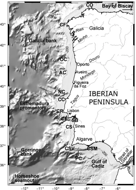
In the case of the North Eastern Atlantic system (Fig. below), the Canary and Iberian regions form two distinct subsystems (Barton 1998). The separation extends beyond geographical characteristics .It is a consequence of the distinctive characteristics of this Northeastern Atlantic region, the discontinuity is imposed by the entrance to the Mediterranean Sea (Relvas et al. 2007).
32 Figure 5: Geography of the Western Iberian system, showing the main features referred to in the text. The 200 m bathymetric contour, that roughly delimits the continental shelf, is represented. From north to south: CO, Cape Ortegal; CF, Cape Finisterre; OC, Oporto Canyon; AC, Aveiro Canyon; NC, Nazare´ Canyon; CC, Cape Carvoeiro; CR, Cape Roca; CE, Cape Espichel; SB, Setu´bal Bay; CS, Cape Sines; CSV, Cape Sa˜o Vicente; PC, Portima˜o Canyon; CSM, Cape Santa Maria.(Relvas et al. 2007)
33 The Azores Current extends eastward separating the oceanic gyre circulation regime into the north (Portugal Current) and the South (Canary Current) (Pollard et al. 1985).It is theorized that the Mediterranean outflow has a dynamic impact in the upper layer of the ocean and may constitute a complimentary mechanism for the formation of the Azores current (Jia 2000).
“The seasonal interplay of the large scale climatology between the Azores high pressure cell, strengthened and displaced northward during the summer, and the Iceland low, weakened at that time, governs the set up of upwelling favourable winds (northerlies) off western Iberia between April and October” (Wooster et al. 1976). There is an association between the separation of the subsystems and the sharp seasonality of the western Iberia system. The author goes on to say that this is also mainly due to the annual cycle of the atmospheric systems.
In the summer months, there is a thermal low over central Iberia, this in turn strengthens the upwelling winds. During the winter periods, the direction of the dominant wind changes and thus poleward flow becomes an outstanding feature at all levels between the surface and the Mediterranean water at approximately 1500 m, along the Iberian shelf edge and slope (Relvas et al. 2007).
The water transported in the surface, poleward flow is relatively warm and saline. This is identifiable in sea surface temperature satellite imagery (Haynes et al. 1990; Peliz et
al. 2005)this extends as far north as the Cantabian coast and the Goban Spur (Pingree
34 The wind regime for this period is reversed, so now it has a southerly component (Frouin et al. 1990),coupled with the meridional density gradient and the continental slope and shelf are attributed to this poleward flow (Peliz et al. 2003).
It is uncertain whether the surface signal of the poleward flow is maintained during the summertime simultaneous with the coastal upwelling jet (Peliz et al. 2005). “The
poleward flow shows a turbulent character, with eddies and smaller scale instabilities typically being generated in the shear regions” (Peliz et al. 2003).
The continental shelf is approximately 610 km wide south of Lisbon, 30–40 km wide off central Portugal and somewhat narrower again off northern Portugal and Galicia (Relvas et al. 2005).According to Relvas et al. (2005) the region is filled with topographic structures such as capes, promontories and submarine canyons with spatial scales from tens to hundreds of kilometres.
The oceanography of this region is largly dominated by medium size structures that represent the “weather” variability of the ocean. The variability of the alongshore windstress is also a major governing factor or coastal circulation (A lvarez-Salgado et
al. 2003) . The oceanographic patterns in the Iberian system reveal a multitude of
structures such as jets, meanders, ubiquitous eddies, upwelling filaments and countercurrents superimposed on the more stable variations at seasonal timescales (Relvas et al. 2005).
35
3.2 Algarve
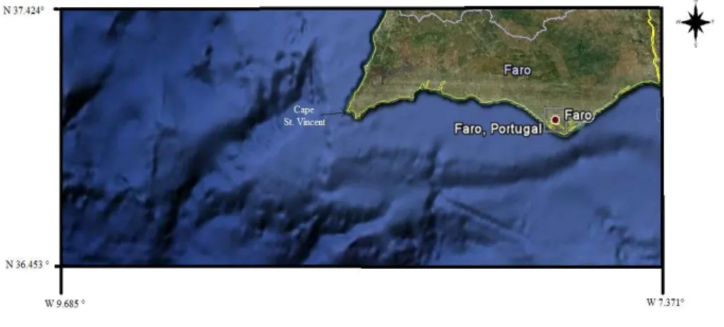
The Algarve is the south-western corner of the Iberian Peninsula. The Algarve Margin is located between 36°–37°N and 7°50–9°25 W. The Algarve coast line stretches about 160 kilometers from the western-most tip to the Spanish border. It is characterized by a rough morphology underlined by the presence of canyons, channels and contourite drifts (Salles et al. 2007).
Figure 6: Showing the study area. (source: Google Earth 2010)
Circulation along the Algarve coast has been the primary subject of several scientific publications. In the last decade these studies have been mainly focuses on surface variability associated with upwelling events (Relvas et al. 2002) also including the Mediterranean Water (MW) Undercurrent(Serra et al. 2005). So far, the actual physical force that generates this counter current has not been identified.
Along the Algarve coast, a coastal counter flow is frequently observed. This is frequently observed in periods of upwelling relaxation, trapped between the coast and a well established upwelling jet (Relvas et al. 2005).The actual physical forcing behind the generation of the counter current is not yet clear. This current is similar to others observed on the California coast and the forcing mechanism may be the spatial
36 variability of upwelling intensity (Harms et al. 1998), wind curl near the coast or a pressure gradient (Ramp et al. 1998) along the coast.
The Portugal Current itself (Martins, 2002; Pérez, 2001) is poorly defined spatially because of the intricate interactions between coastal and offshore currents, bottom topography, and water masses. The system is comprised of the following main currents: The Portugal Current, which is a broad, slow, generally southward-flowing current that extends from about 10°W to about 24°W longitude;
The Portugal Coastal Counter current (PCCC), a southward flowing surface current along the coast during down welling season, mainly over the narrow continental shelf to about 10-11°W longitude and flow from about 41-44°N;
The Portugal Coastal Current (PCC), a generally poleward current that dominates over the PCCC during times of upwelling and like the PCCC, extends to about 10-11°W from shore, also present mainly from 41-44°N, where flow is 13.5 ± 5.7 cm s-1 (Pérez
et al. 2001; Martins et al. 2002). The Portugal current as represented by the Mariano Global Surface Velocity Analysis (MGSVA). The average flow is towards the south and feeds the Canary Current.
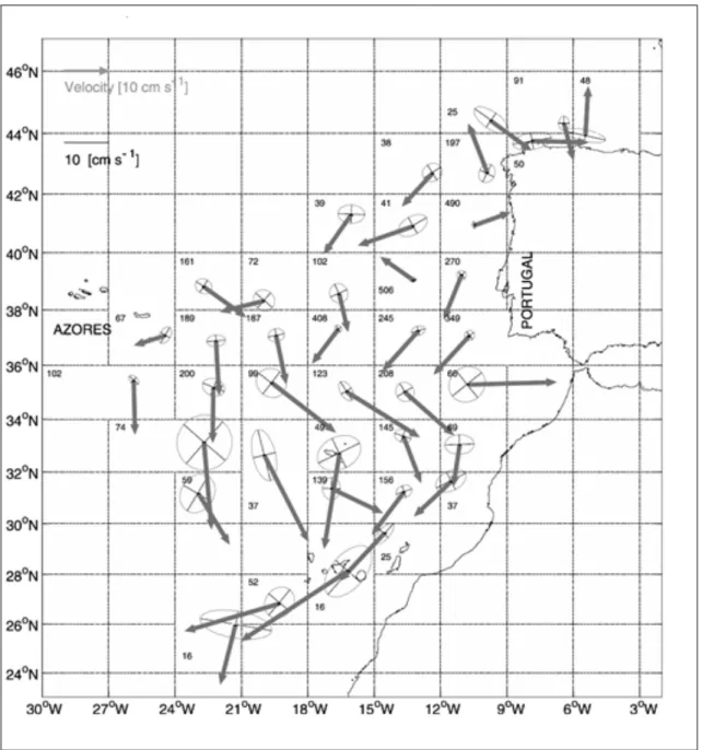
Figure 7 below shows the average velocity field in the northeast Atlantic as derived from near-surface drifters. The arrow’s origin is located at the average drifter positions in each box, and its length is directly proportional to the velocity magnitude. The ellipses indicate the principal directions of variance, and the correspondent axes indicate the errors. The arrow corresponding to a 10 cm s_1 mean velocity and a linear segment of 10 cm s_1 for the error are indicated on top of the figure. The number of drifter days
37 used in the averages is indicated on the upper left corner of each box whose geometry is variable in order to improve statistical reliability(Martins et al. 2002).
Figure 7 Surface Circulation on The Eastern North Atlantic (Martins et al. 2002)
The Portugal currents, has the mean pattern as well as seasonal variation and are well established despite relatively few systematic observations. The Portugal and Canary
38 Generally, the mean flow on the surface is southward, however seasonal winds in the region can result in both northward and southward flows, which were observed with drifters equipped with holey sock drogues centred at about 15 m over a period of 14.4 years (Martins et al. 2002)
3.2.3 Tidal Regime
The tidal regime is semidiurnal and mesotidal with tides ranging from 2.70 to 1.36 m during neap tides and from 3.82 to 0.64 m during spring tides (Vilamoura tide gauge). The mean rate of relative sea-level rise has been estimated as 1.5 ± 0.2 mm/yr according to data from the Lagos tide gauge's series registered between 1908 and 1987 (Dias et al. 1992 ; Moura et al. 2006).
3.2.4 Upwelling
Predominant trade winds from the north, cause wind driven upwelling along the coast of the Iberian Peninsula during the summer months. Cooler water from depths of 100-300 m is upwelled (Smyth et al. 2001; Bischof et al. 2003).These events usually begin around and are particularly intense off of Cape Finisterre and Cabo da Roca, often forming filaments that can reach as far as 100 km westward (Cuehlho et al. 2002; Huthnance et al. 2002; Bischof et al. 2003)and their velocities, tracked by thermal features in satellite images, can reach up to 0.28 m s -1 (Smyth et al. 2001) .
39 Studies of Upwelling in the Portuguese coastline have been done and papers have been published on the same topic by authors such as (Relvas et al. 2002; Sofia et al. 2005; Santos et al. 2001). Upwelling responds quickly to northerly winds, particularly south of capes, appearing first along the coastline and then spreading offshore as the event progresses (Fiúza 1983).
The Portugal Coastal Countercurrent (PCCC) during times of upwelling and like the PCCC, extends to about 10-11°W from shore, also present mainly from 41-44°N, where flow is 13.5 ± 6 5.7 cm s-1 (Pérez et al. 2001; Solignac et al. 2008) . The Portugal Current system is supplied mainly by the intergyre zone in the Atlantic, a region of weak circulation bounded to the north by the North Atlantic Current and to the south by the Azores Current (Pérez et al. 2001). For some part of the year the north-east Trade Winds blow along every part of the subtropical Eastern boundary with a strong alongshore component that produces offshore Ekman transport in the surface layers and therefore upwelling at the coast (Barton 2001).
The strength of upwelling is conventionally expressed in terms of the upwelling (or Bakun) index, which is simply the Ekman transport
Equation 28
where q is the component of wind stress parallel to shore, o is the density of sea water, f is the Coriolis parameter (Barton 2001) refer to figure below.
40 Figure 8 : Showing coastal upwelling along the Sagres coastline SW-Portugal
(Source Microbiology procedure (http://www.microbiologyprocedure.com/microbial-ecology-of-differentecosystems/marine-ecosystem-upwelling.html) accessed07/05/2010
Oceanographers have long sought to verify the theoretical Ekman transport relation, which predicts that a steady wind stress acting together with the Coriolis force will produce a transport of water to the right of the wind (Price et al. 1987).
Off the coast of Portugal, upwelling can be found south of 40º N during summer and autumn; between 40ºN and 43ºN the upwelling period decreases with increasing latitude. The yearly amplitude of differences of sea level pressure normal to the coast which represents the synoptic scale coast parallel wind component and offshore surface temperatures is largest in 38ºN, decreasing to the north. From empirical orthogonal functions it is suggested that off Portugal local winds induce a more intense upwelling than the winds off Northwest Africa (Detlefsen et al. 1980) Local winds, the continental-shelf/upper-slope bathymetry and the coastal morphology largely determines the upwelling patterns off Portugal (Fiúza 1983).
Sousa et al (1992) concluded that upwelling took place seasonally along the west coast of Portugal. Upwelling would reach its maximum in July, August and September. This
41 usually occurs under fairly steady northly winds ands that its intensity presented a strong correlation with the north-south wind stress.
3.3 Cape St. Vincent
The western Iberian Peninsula (IP) is located in the northern limit of the Eastern North Atlantic Upwelling Region. Geographically, the zone is characterized by the presence of Cape St. Vincent, where the western and southern coasts intersect at an almost right angle. This cape is the most south-western point in Portugal .The 25 km wide southern shelf slopes gently down to a sharp edge at 100–130 meters depth, defined by a sudden step down to the 700 m contour. This pronounced feature extends around the southwest tip of Portugal, reaching about 10 km north of Cape St. Vincent. The shelf off the west coast of Algarve is steep and only 10 km wide (Leal 2005).
The oceanographic system off of the south-western Iberian Peninsula is still not very detailed. This system forms part of the northern tip of the Eastern Boundary Current System (EBCS) of West Europe and Northern Africa. The abrupt coastline changes at Cape Finisterre and Cape St. Vincent introduce a source for sharp geographical shifts that have an influence on the oceanographic setting.
At these sites the west coast interacts almost at right angles with the North and South Iberian coasts respectively, which confers a particular meridional symmetry in this region. This meridional symmetry is also observed with the existence of two large bights where vivid recirculation’s occur, namely the Gulf of Cadiz at the south (Sanchez
et al. 2003) and the Bay of Biscay at the north (Pingree et al. 1990; Leal 2005).
Sanchez and Relvas (2003) presented a comprehensive review about the average summer circulation. They noted that during the summer season there is an upwelling of colder subsurface eastern North Atlantic Central Water over the shelf and slope. Their
42 transport analyses observe that at times, the equatorward upwelling jet sometimes had a vigorous interaction with the offshore circulation.
Leal (2005) inferred that there were two man mechanisms: one associated with recirculation of 0.6 Sv (1 Sv=106 m3s−1) with a northern branch of the Azores Current in the vicinity of Cape St. Vincent; the other consists of cross-shelf exchanges effected by persistent upwelling filaments.
Work based on scatterometer winds have evidenced strong similarity of the winds that fall within the vicinity of the most prominent capes along the Iberian Peninsula, Cape Finisterre (Torres et al. 2003) and Cape St. Vincent.
The seasonal alteration of wind driven flows in the upper surface (400m), is a characteristic of the ocean. Sanchez et al(2003) showed proof of the mesoscale nature of flows in the western Iberian Peninsula, in summertime and in winter (Peliz et al. 2005).
The classical view of upwelling circulation is also featured in the climatological features (Sanchez et al. 2003).A cold upwelling jet extending over the upper 100 meter or more of the water column advects 1 Sv of low-salinity water equatorward.
This climatological circulation also revealed interplay between the offshore field and the pure upwelling circulation. The recurrent activity of upwelling filaments are one of the most active mechanisms in the system. Upwelling filaments are cold-water tongues, with source in the upwelling zone. They may reach some 50 km of width and several hundreds of km of length (Leal 2005).