U
NIVERSIDADE DO
A
LGARVE
Faculdade de Ciˆencias e Tecnologia
Real-time path and obstacle
detection for blind persons
Jo˜ao Tiago Pereira Nunes Jos´e
Mestrado em Engenharia Inform´atica
U
NIVERSIDADE DO
A
LGARVE
Faculdade de Ciˆencias e Tecnologia
Real-time path and obstacle
detection for blind persons
Jo˜ao Tiago Pereira Nunes Jos´e
Mestrado em Engenharia Inform´atica
2010
Dissertac¸˜ao orientada por:
Resumo
Nesta dissertac¸˜ao s˜ao apresentados algoritmos de vis˜ao computacional, os quais fazem parte de um prot ´otipo direccionado a ajudar na mobilidade de pessoas com dificuldades visuais. O seu objectivo ´e servir de aux´ılio ao seu utilizador na navegac¸˜ao interior e exterior, ao detectar o caminho dentro do qual este pode “confortavelmente” andar, de forma a evitar que este saia do seu trajecto, como por exemplo em passeios ou corredores, bem como ao detectar obst´aculos que se encontrem no trajecto que este pretende seguir, ao fornecer indicac¸ ˜oes da melhor forma para os evitar. O desenvolvimento deste prot ´otipo encontra-se integrado no projecto SmartVision, financiado pela Fundac¸˜ao para a Ciˆencia e Tecnologia, com a referˆencia PTDC/EIA/73633/2006.
Inicialmente ´e descrito o algoritmo de detecc¸˜ao de caminhos, o qual consiste numa vers˜ao adaptada da transformada de Hough, e cujo intuito ´e o de detectar as bordas que correspondem aos limites do caminho, sendo estas as linhas com maior continuidade na parte inferior da imagem relativamente `a linha do horizonte, ou seja, a metade mais perto do ch˜ao. A linha do horizonte ´e definida como uma linha horizontal, cuja posic¸˜ao: (a) na fase de inicializac¸˜ao se situa no centro da imagem; (b) ap ´os a inicializac¸˜ao corresponde `a intersecc¸˜ao dos limites calculados para as imagens anteriores. Mais concretamente, este algoritmo ´e aplicado sobre o resultado do detector de arestas Canny, o qual nos d´a uma imagem bin´aria relativamente `a presenc¸a de arestas significativas na mesma. Este algoritmo tem uma fase de inicializac¸˜ao, a qual ´e usada para restringir a regi˜ao de procura dos referidos limites no espac¸o de Hough, tendo como benef´ıcios o uso de menos processamento, bem como o de obter limites mais precisos. Isto, tendo em conta que um utilizador caminha normalmente a uma velocidade de 1 m/s, e que os fotogramas s˜ao obtidos a uma taxa de pelo menos 5 fps, o que significa que, no m´ınimo, uma imagem ´e adquirida a cada 20 cm de movimento.
De seguida explicam-se os algoritmos de detecc¸˜ao de obst´aculos, os quais visam verificar se existem obst´aculos presentes `a frente do utilizador, para que o mesmo possa evit´a-los durante o seu percurso.
em que se verificam as derivadas horizontais e verticais para cada linha e coluna respectivamente. Este consiste numa variac¸˜ao do conhecido algoritmo Zero Crossing, em que s˜ao somadas as amplitudes entre os m´aximos e m´ınimos a cada vez que o valor da derivada muda o sinal (positivo ou negativo). Existe um valor limiar, o qual ´e actualizado durante o decorrer da sequˆencia de v´ıdeo.
O segundo algoritmo de detecc¸˜ao de obst´aculos baseia-se, mais uma vez, na detecc¸˜ao de arestas (Canny), no qual se diferenciam as arestas orientadas horizon-talmente das orientadas verticalmente. S˜ao ent˜ao definidos histogramas para as arestas horizontais e verticais, de forma a definir uma regi˜ao de intersecc¸˜ao utilizada para localizar o obst´aculo, atrav´es da multiplicac¸˜ao dos histogramas resultantes. Um histograma resulta da soma coluna a coluna das arestas horizontais, outro da soma linha a linha das arestas verticais. Os valores limiar deste algoritmo s˜ao tamb´em actualizados durante a sequˆencia de v´ıdeo, quando n˜ao existem obst´aculos detectados. Estes valores alteram os habitualmente usados no referido detector de arestas Canny, de forma a ajustar os mesmos `a magnitude m´axima resultante de cada tipo de textura (tipo de revestimento do ch˜ao).
Relativamente ao terceiro algoritmo, est´a relacionado com diferenc¸as de texturas na imagem, tendo como base as m´ascaras de textura de Laws. Uma combinac¸˜ao destas m´ascaras ´e usada para que uma variac¸˜ao significativa na textura, de uma parte da imagem, possa ser considerada como um obst´aculo. S˜ao utilizadas 4 das 25 m´ascaras de Laws, respectivamente E5L5, R5R5, E5S5 e L5S5, as quais resultam em filtragens mais significativas para o fim pretendido, obtendo-se assim uma melhor discriminac¸˜ao entre v´arias texturas sem comprometer o desempenho. Os valores resultantes s˜ao ent˜ao normalizados relativamente ao valor m´ınimo e m´aximo para cada m´ascara, de forma a uniformizar a contribuic¸˜ao resultante de cada filtragem. Como nos restantes algor´ıtmos, existe um valor limiar actualizado durante o movi-mento do utilizador, o qual ´e ajustado ao tipo de textura do pavimovi-mento, para que seja poss´ıvel diferenciar a mesma da textura de obst´aculos, assim contribuindo para a sua detecc¸˜ao.
Estes trˆes algoritmos s˜ao combinados de forma a confirmarem a presenc¸a de um obst´aculo na imagem. O utilizador ´e alertado da existˆencia do mesmo apenas
quando, em pelo menos trˆes imagens consecutivas na sequˆencia de v´ıdeo a regi˜ao de intersecc¸˜ao de pelo menos dois algoritmos de detecc¸˜ao n˜ao ´e vazia. Ao verificar-se o espac¸o dispon´ıvel entre os limites do caminho e o obst´aculo detectado, o utilizador ´e instru´ıdo da melhor forma a permanecer no seu trajecto e contornar o obst´aculo. Esta decis˜ao ´e tomada tendo em conta o maior espac¸o sem obst´aculos dentro do caminho detectado.
Todos os algoritmos apresentados s˜ao extremamente leves computacionalmente, pelo que podem ser utilizados num netbook de baixo custo com uma cˆamara de v´ıdeo Web com uma resoluc¸˜ao VGA (640x480). Testes efectuados demonstram que um netbook de gama m´edia ´e capaz de analisar os fotogramas adquiridos numa sequˆencia de v´ıdeo, a uma taxa superior a 5 fps.
Existe tamb´em a possibilidade de aplicar os referidos algoritmos num software para telem ´ovel/smartphone. O desempenho destes dispositivos, a n´ıvel computa-cional, est´a a crescer largamente, pelo que se torna pouco dispendioso e cada vez mais acess´ıvel adquirir um modelo com poder computacional suficiente para uma aplicac¸˜ao do g´enero. Em relac¸˜ao `a cˆamara, ´e muito habitual neste tipo de dispos-itivos existir uma integrada, em que na grande maioria a resoluc¸˜ao da mesma ´e suficiente para aplicar os referidos algoritmos, pelo que se evita assim a utilizac¸˜ao de um dispositivo adicional. A usabilidade deste tipo de dispositivo ´e tamb´em muito pr´atica, podendo ser utilizado mais frequentemente pendurado ao pescoc¸o `a altura do peito, ou mesmo segurando o dispositivo quando necess´ario para uma utilizac¸˜ao menos frequente. Os alertas podem ser instru´ıdos sonoramente pelo altifalante integrado, bem como atrav´es do uso de apenas um auricular, ou ainda sinalizado pelo modo de vibrac¸˜ao do dispositivo.
Deste trabalho encontram-se publicados, `a data, 2 artigos em revista e 2 em conferˆencia, os quais referenciados em [1], [2], [3] e [4]. Aguarda revis˜ao um 5º artigo submetido para conferˆencia, ao qual se faz referˆencia em [5].
Abstract
In this thesis we present algorithms that can be used to improve the mobility of visually impaired persons. First we propose an algorithm to detect the path where the user can walk. This algorithm is based on an adapted version of the Hough transform, in which we apply a method for gathering the most continuous path borders after an edge detector is applied. After an initialization stage we dynamically restrict the area where we look for path borders. This improves accuracy and performance, assuming that the positions of the borders in successive frames are rather stable: images are gathered at a frame rate of at least 5 fps and the user walks at a speed of at most 1 m/s. Other algorithms serve obstacle detection, such that the user can avoid them when walking inside the detected walkable path. To this purpose an obstacle detection window is created, where we look for possible obstacles. The first algorithm applied is based on the zero crossings of vertical and horizontal derivatives of the image. The second algorithm uses the Canny edge detector, separating vertically and horizontally oriented edges to define a region where an obstacle may be. The third algorithm uses Laws’ texture masks in order to verify differences in the ground’s textures. Dynamic thresholds are applied in all algorithms in order to adapt to different pavements. An obstacle is assumed present if the intersection of the regions detected by at least two of the three algorithms is positive in at least three consecutive frames. The algorithms can be used on a modern “netbook” at a frame rate of at least 5 fps, using a normal webcam with VGA resolution (640x480 pixels).
Declaration of authenticity
No portion of the work referred to in this thesis has been submitted in support of an application for another degree or qualification of this or any other university or other institute of learning. To the best of my knowledge and belief, this thesis contains no material previously published or written by another person, except where due reference has been made.
Acknowledgements
First of all I would like to thank Prof. Dr. Hans du Buf for his inspiring work and knowledge, which lead me to contribute to this project, for all the advices, supervision, comprehension and availability.
For the leisure moments, helping each other, and mainly for the good environ-ment and team spirit I would also like to thank all of my laboratory colleagues. To Jo˜ao Rodrigues, Roberto Lam, Jaime Martins, Miguel Farrajota and to all the non-permanent members that have gone through our lab, I thank them all. A special gratitude goes to Jo˜ao Rodrigues, for all the ideas, time and patience, which he was always willing to share.
To my fianc´ee Inˆes Seruca, for all the love and cherishing, comprehension and patience, and mainly for her encouragement, providing me the home environment needed to work on this thesis.
A special thanks to my parents, Cesaltina Viegas and Rui Jos´e, to my brothers Rui and Diogo Jos´e, without whom I would not be who I am today. Also to my whole family: aunts, uncles, cousins, grandfathers, grandmothers. . . to every one, a special thank you.
Contents
Resumo i Abstract iv Declaration of authenticity v Acknowledgements vi 1 Introduction 11.1 Motivation and scope . . . 1
1.2 Thesis contribution . . . 4
1.3 Thesis overview . . . 5
2 Background 6 3 Path detection 10 3.1 Introduction . . . 10
3.2 Path detection window (PDW) . . . 11
3.3 Pre-processing . . . 13
3.4 Adapted Hough Space (AHS) . . . 14
4 Obstacle detection 24
4.1 Introduction . . . 24
4.2 Obstacle detection window (ODW) . . . 24
4.2.1 Window size . . . 25
4.2.2 Correction of perspective projection . . . 28
4.2.3 Image pre-processing . . . 29
4.3 Zero crossing counting algorithm . . . 30
4.3.1 Horizontal and vertical first derivative . . . 31
4.3.2 Zero crossing counting . . . 31
4.3.3 Thresholding and final region detection . . . 32
4.4 Histograms of binary edges algorithm . . . 34
4.4.1 Horizontal and vertical edges . . . 35
4.4.2 Thresholding and final result . . . 35
4.5 Laws’ texture masks algorithm . . . 37
4.5.1 Laws’ masks feature extraction . . . 37
4.5.2 Thresholding and final result . . . 38
4.6 Obstacle avoidance . . . 39
5 Results 41
6 Conclusions 47
Chapter 1
Introduction
1.1
Motivation and scope
Worldwide there are about 40 million blind people, plus more than 150 million with severe visual impairments1. Most must rely on the white cane for local navigation,
constantly swaying it in front for negotiating walking paths and obstacles in the immediate surround. Technologically it is possible to develop a vision aid which complements the white cane, for alerting the user to looming obstacles beyond the reach of the cane, but also for providing assistance in global navigation when going to a certain destination. However, since more than 80% of potential users of such an aid are from so-called developing countries with low economic level, most are very poor and cannot afford expensive solutions. Even guide-dogs cannot be afforded by most because of their expensive training.
A vision aid should replace a big part of the functionality of a normal visual sys-tem: centering automatically on paths, detecting static and moving obstacles on the fly, and guiding to a destiny like a shop which is already visible. This functionality can nowadays be extended by global navigation, using GPS (Global Positioning System) in combination with a GIS (Geographic Information System). For indoor localisation and navigation, passive and active RFID (Radio Frequency
cation) tags can be used, also “indoor localisation” based on WiFi access points as developed by NOKIA; see [6]. However, active and real-time computer vision algorithms are demanding in terms of CPU power, and the seamless integration with GPS/WiFi/GIS will demand even more CPU power. Luckily, CPU power of portable computers is rapidly increasing, and many devices are already equipped with WiFi and GPS.
The Portuguese project “SmartVision: active vision for the blind”, financed by the Portuguese Foundation for Science and Technology2, combines several
technologies, such as GPS, GIS, Wi-Fi and computer vision, to create a system which assists the visually impaired navigate in- and outdoor [4]. Its goal is to develop a vision and navigation aid which is: (a) not expensive, such that it can be afforded by many blind persons, although at the moment only in “developed” countries; (b) easily portable, not being a hindrence when walking with the cane; (c) complementing the cane but not substituting it; (d) extremely easy to use in terms of intuitive interfacing; and (e) providing assistance in local and global navigation in real-time.
This thesis focuses on the local visual functionality only. For aspects related to GPS, WiFi or GIS, see [4]. The diagram in Fig. 1.1 shows the “local vision module” components. This thesis is only about path detection and static obstacles as shown in red. Frame stabilisation using egomotion and detection of moving obstacles using optical flow is explained in [7]. Stereo disparity is used to estimate the distance of the user to an obstacle. An audio interface for alerting the blind user to incorrect path centering and to static as well as moving obstacles is also being developed. This can be done using sinewave sounds with higher or lower pitch and amplitude, and the intervals between periodic beeps can change according to an obstacle’s distance. Speech synthesis can be used instead of or to complement the previously described sounds. Voice recognition for interacting with the device is also an option. The main objective here is to develop algorithms for path and obstacle detection, like boxes, poles and missing cobblestones. The algorithms described in this thesis are devoted to paths and static obstacles. Moving obstacles are dealt with in another
Figure 1.1: Local vision module scheme of the SmartVision prototype. MSc. thesis [7], but are already integrated in a first prototype of the system.
A previous paper [8] presented an initial detection method for paths with fixed obstacles. The system first detects the path borders, using edge information in combination with a tracking mask, to obtain straight lines with their slopes and the vanishing point. Once the borders are found, a rectangular window is defined within which two obstacle detection methods are applied. The first determines the variation of the maxima and minima of the grey levels of the pixels. The second uses the binary edge image and searches in the vertical and horizontal edge histograms for discrepancies in the number of edge points. Together, these methods allow to detect possible obstacles with their position and size, such that the user can be alerted and informed about the best way to avoid them.
and robust, also dealing better with pavement textures, even detecting obstacles in multi-textured pavements. All algorithms are also faster, thus lowering the usage of computer resources.
1.2
Thesis contribution
This thesis focuses on the feasibility of algorithms to implement a guidance system which improves the mobility of a blind person. These algorithms should use the least computer resources possible in order to run on a lightweight and low-cost device.
Blind people should be able to use this device without interfering it with their “normal” navigation. The device will alert the person to obstacles present on his path, and a way to bypass them. This is enabled by the detection of the walkable path, i.e., where the user can walk safely. After the path borders are detected, the device will be able to guide the person in order to avoid obstacles in front. Also, it should warn the user in case his trajectory will take him off the walkable path he is on.
As many obstacles cannot be detected with the use of the cane, e.g., small obstacles and irregularities on the ground such as loose stones, etc, our system can improve mobility not just by warning in advance of appearing obstacles, but also by detecting obstacles that would not be noticed with the cane.
Independently of the algorithms and regarding usage, easy portability is a priority. In the scope of the SmartVision project a stereo camera and a netbook are used, but it is also possible to use a mobile device such as a smartphone, which nowadays achieves more computing power. Also, most mobile phones include now an integrated camera with more than enough resolution for this kind of application. Using it permanently, hanged from the neck at chest height, and only occasionally grabbed for a telephone call, this is a very portable and off-the-shelf solution. However, in the scope of this thesis we will use the stereo camera and the netbook as stated earlier.
1.3
Thesis overview
The structure of this thesis is roughly based on the chronological development, as follows:
• First an overview of existing approaches is presented in Chapter 2. This covers the context of the SmartVision project and more focused approaches in the context of this thesis;
• Path detection is dealt with in Chapter 3, which explains how the user can stay on the path, avoiding rough terrain and, later, obstacles;
• In Chapter 4 the obstacle detection algorithms are explained: the first one is based on horizontal and vertical first derivatives, the second uses the Canny edge detector, and the third one employs Laws’ masks to extract texture information from the image;
• Experimental results obtained with real video sequences are presented in Chapter 5, with a detailed explanation of each sequence;
• A discussion concludes this thesis in Chapter 6, where the global achievements are explained.
Chapter 2
Background
There are several approaches to developing devices for helping the visually im-paired. Some of these approaches are presented below.
One system for obstacle avoidance is based on a hemispherical ultrasound sensor array [9]. It can detect obstacles in front and unimpeded directions are obtained via range values at consecutive times. The system comprises an ARM9 embedded system, the sensor array, an orientation tracker and a set of pager motors. The KASPA system [10] is also based on ultrasonic sensors. The distance to an obstacle is conveyed to the user by sound codes. Binaural technology can be used to guide users toward environmental landmarks, as used in [11], where GPS data are translated into useful information for a blind user.
Talking Points [12] is an urban orientation system based on electronic tags with spoken (voice) messages. These tags can be attached to many landmarks like entrances of buildings, elevators, but also bus stops and buses. A push-button on a hand-held device is used to activate a tag, after which the spoken message is made audible by the device’s small loudspeaker.
iSONIC [13] is a travel aid complementing the cane. It detects obstacles at head-height and alerts by vibration or sound to dangerous situations, with an algorithm to reduce confusing and unnecessary detections. iSONIC can also give information about an object’s colour and environmental brightness.
The GuideCane [14] is a computerised travel aid for blind pedestrians. It consists of a long handle and a “sensor head” unit that is attached at the distal end of the handle. The sensor head is mounted on a steerable, two-wheeled steering axle. During operation, the user pushes the lightweight GuideCane in front. Ultrasonic sensors mounted on the sensor head detect obstacles and steer the device around them. The user feels the steering as a noticeable physical force through the handle and is able to follow the GuideCane’s path easily and without any conscious effort.
Drishti [15] is an in- and outdoor blind navigation system. Outdoor it uses DGPS as its location system to keep the user as close as possible to the central line of sidewalks; it provides the user with an optimal route by means of its dynamic routing and re-routing ability. The user can switch the system from outdoor to indoor environment with a simple vocal command. An ultrasound positioning system is used to provide precise indoor location measurements. The user can get vocal prompts to avoid possible obstacles and step-by-step walking guidance to move about in an indoor environment.
Cognitive Aid System for Blind People (CASBliP) [16] was a European project with seven partners. It aimed at developing a system capable of interpreting and managing real-world information from different sources to support mobility-assistance to any kind of visually impaired persons. Environmental information from various sensors is acquired and transformed, either into enhanced images for visually impaired people, or into acoustic maps presented by headphones for blind people. Two prototypes have been developed for the validation of the concepts: a) an acoustic prototype, containing a novel time-of-flight CMOS range image sensor and an audio interface for transforming distance data into a spatial sound map; b) a real-time mobility assistance prototype, equipped with several environmental and user interfaces, controlled by a portable PC, to enable users to navigate safely in in-and outdoor environments.
SWAN, System for Wearable Audio Navigation, is a project of the Sonification Lab at Georgia Institute of Technology [17]. The core system is a wearable computer with a variety of location- and orientation-tracking technologies including, among others, GPS, inertial sensors, pedometer, RFID tags, RF sensors, and a compass.
Sophisticated sensor fusion is used to determine the best estimate of the user’s location and which way he or she is facing.
Tyflos-Navigator, a wearable navigation system, deals with the development of a wearable device which consiste of dark glasses with 2 cameras, a portable computer, microphone, ear-speaker, 2D vibration array, etc. It captures images from the surrounding environment, converts them into 3D representations and generates vibrations (on the user chest) associated with the distances of the user’s head to surrounding obstacles, see e.g. [18]. The same authors in [19] presented a detailed discussion of other relevant projects with navigation capabilities.
A multi-sensor strategy based on an IR-multisensor array is presented in [20]. It employs smart signal processing to provide the user with suitable information about the position of objects hindering his or her path. The authors in [21] present an obstacle detection system with multi-sonar sensors which sends vibro-tactile information to the user with the obstacle’s position.
A computer vision system for blind persons in a wheelchair is presented in [22]. The system collects features of nearby terrain from cameras mounted rigidly to the wheelchair. It assists in the detection of hazards such as obstacles and drop-offs ahead of or alongside the chair, as well as detecting veering paths, locating curb cuts, finding a clear path, and maintaining a straight course. The resulting information is intended to be integrated with inputs from other sensors and communicated to the traveler using synthesised speech, audible tones and tactile cues.
More related to computer vision is a method to detect the borders of paths and sidewalks, see e.g. [23]. A different approach, using monocular colour vision, is presented in [24]. Pixels are classified as part of the ground, or if not as being an obstacle that should be avoided. Color histograms can also be used for side-walk following, as shown in [25], using hue and saturation histograms for pixel classification.
Sidewalk or curb detection, but limited to short distances, can be achieved with the use of a laser stripe as described in [26]. Other computer-vision techniques [27, 28] use the Hough Transform to form candidate clusters of lines to detect sidewalks. In [29], a weighted Hough Transform is used for detecting locations
of curb edges. Later, using a commercial stereo vision system combined with brightness information, curbs and stairways are precisely detected [30].
Concerning detection of vanishing points, two methods are presented in [31]: one using a probabilistic model operating in polar space, and a second using a deterministic approach directly in Cartesian space, the latter being computationally lighter and also more reliable. For computing the horizon line, a different approach using a dense optical flow is presented in [32].
Chapter 3
Path detection
3.1
Introduction
In this chapter the path detection algorithm is presented. The goal is to locate the user inside the walkable path, i.e, the area where the user can walk safely. There will be a left and a right border which intersect at a point called the vanishing point (VP); see Section 3.2. The vanishing point is used to select the part of the image which is used for the detection of the borders, i.e., below the VP where the borders should be. After pre-processing using the Canny edge detector (Section. 3.3), an adapted version of the Hough transform is applied to extract the left and right borders from the image as detailed in Section 3.4. In Section 3.5 we show how to get the path window from the original image.
From this point on we will refer to an image as I, to a line as L, to a point as P and to a set of points as S. The width of an image will be refered to as W(I) and the
height as H(I), whereas x(I) and y(I)are coordinates in I.
All used images were captured at Gambelas Campus of the University of the Algarve, using the Bumblebee®2 from Point Grey Research Inc., the same camera
as used in the SmartVision project. This camera is fixed to the chest of the user, pointing forward with the image plane being vertical, at a height of about 1.5 m from the ground (this depends a bit on the height of the user, but it is not relevant to the
system’s performance). Results presented here are obtained by using only the right-side camera, and the system performs equally well using a normal, inexpensive webcam with about the same resolution. Even a mobile phone camera can be used, as nowadays most models integrate a VGA or better camera. The resolution must be sufficient to resolve textures of pavements and potential obstacles like holes with a minimum size of 10 cm at a distance of 2 to 5 meters from the camera.
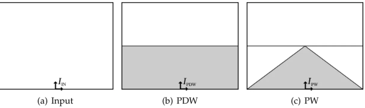
We start by using an input frame to determine the path detection window, or PDW, where we will search for the path borders. This results in the path window (PW), which is the area where the blind can walk safely. These are illustrated in Fig. 3.1.
(a) Input (b) PDW (c) PW
Figure 3.1: Path detection stages with coordinate axes.
3.2
Path detection window (PDW)
The frames of the camera (vertically aligned, thus pointing forward) contain in the lower part the borders of the path which the user is on, i.e., the area that we need to analyse. In this bottom part we define the path-detection window or PDW.
Let IIN(xIN, yIN)denote an input frame with fixed width WINand height HIN. Let
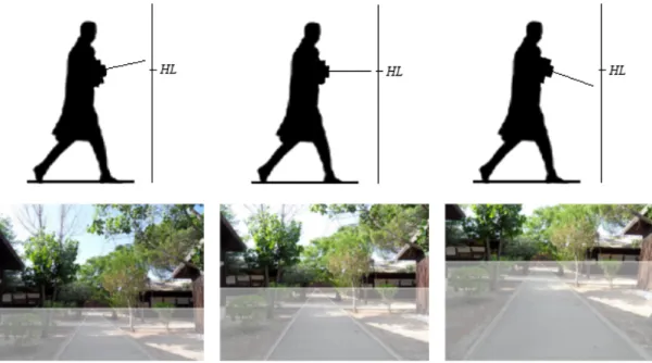
HL denote a horizon line close to the middle of the frame. If the camera is exactly in the vertical position, then yHL = HIN/2. If the camera points lower or higher, HL
will be higher or lower, respectively; see Fig. 3.2.
Figure 3.2: From left to right: camera pointing up, vertically aligned, and pointing down. The corresponding path detection windows are highlighted in the images. straight lines in the lower half of the frame, delimited by HL. The area below HL is where we will look for the path borders, which we call IPDW. Examples of IIN
and IPDWare presented in Fig. 3.2 with the PDW highlighted. Figure 3.3 also shows
the PDW with the HL and detected path borders. The coordinate axes are shown in Fig. 3.1: (a) input image, (b) path detection window, and (c) the resulting path window which will be further processed.
Because of perspective projection, the left and right borders of the path and many other straight structures intersect at the vanishing point VP. Since vertical camera alignment is not fixed but varies over time when the user walks, we use the VP in order to determine the line: yHL = yVP. Consequently, the path detection window is
defined by IPDW(xPDW, yPDW)with xPDW ∈ [−WIN/2, WIN/2−1]and yPDW ∈ [0, yVP],
if the bottom-centre pixel of each frame is the origin of the coordinate system. Different PDWs are illustrated in Figure 3.2.
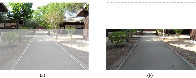
(a) (b)
Figure 3.3: (a) the original image with the path borders, the horizon line, and the PDW area highlighted; (b) the original image reduced to the PDW.
previous five frames: for yVP,i, i.e., frame number i which still must be analysed,
yVP,i = (
Pi−1
j=i−5yVP,j)/5. This cannot be done in the case of the first five frames,
for which we use the bottom half part of the image, or yVP = HIN/2, assuming
approximately vertical camera alignment. This is not a problem because the first five frames are mainly used for system initialisation and a frame rate of 5 fps implies only one second.
3.3
Pre-processing
The Canny edge detector in combination with an adapted version of the Hough transform are applied to IPDW, in order to detect the borders and the vanishing point.
In order to reduce CPU time, only greyscale information is processed after resizing each frame to a width of 300 pixels, using bilinear interpolation, maintaining the aspect ratio. Then two iterations of a 3x3 smoothing filter are applied in order to suppress noise. The Canny edge detector [33] is applied with σ = 1.0, which defines the size of the Gaussian filter, in combination with TL = 0.25and TH = 0.5which
are the low and high thresholds for hysteresis edge tracking. The result is a binary edge image IP(xP, yP), of width WP = 300and height HP= 300 × (HPDW/WPDW),
with xP ∈ [−WP/2, WP/2 − 1]and yP ∈ [0, HP− 1]. Figure 3.4 shows one original
frame together with the greyscale version, then the resized and lowpass-filtered ones, plus detected edges. The last three images are a part of the original image.
(a) Original image (b) Grayscale image
(c) Resized image (d) Smoothed image (e) Canny edge image
Figure 3.4: An input frame (a) is converted to greyscale (b), then cut and resized (c), smoothed (d) before edge detection (e).
3.4
Adapted Hough Space (AHS)
In this section we explain the adapted version of the Hough transform used for detecting the left and right border lines. The AHS is built from the pre-processed image as in Fig. 3.4(e), where we have the edge map. From this we need to extract continuous lines, which are the most probable border candidates. Using sequences of frames, the accuracy of the lines’ locations can be improved. As the Hough space is restricted to a smaller window, this also results in a lower computational cost.
The borders of paths like sidewalks and corridors are usually found in pairs: one to the left and one to the right, assuming that the path is in the camera’s field of view; see e.g. Fig. 3.4(a). The case where one or both borders are not found in the image is
explained later. We use the Hough transform [34], where ρ = x × cos θ + y × sin θ, to search for straight lines in the left and right halves of the binary edge image IPfor
border candidates, also assuming that candidates intersect at the vanishing point.
Figure 3.5: Edge image after pre-processing with the reference system. For finding the left and right borders, the Hough transform is applied to IP,
yield-ing the Adapted Hough Space IAHS(ρ, θ). The values of ∆θ and ∆ρ are explained
below. Figure 3.5 shows the image we will use as an example.
With the purpose of maximising the number of searched lines, and minimising the computation time, we calculate the intervals for θ and ρ in such a way that we do not miss or repeat any lines.
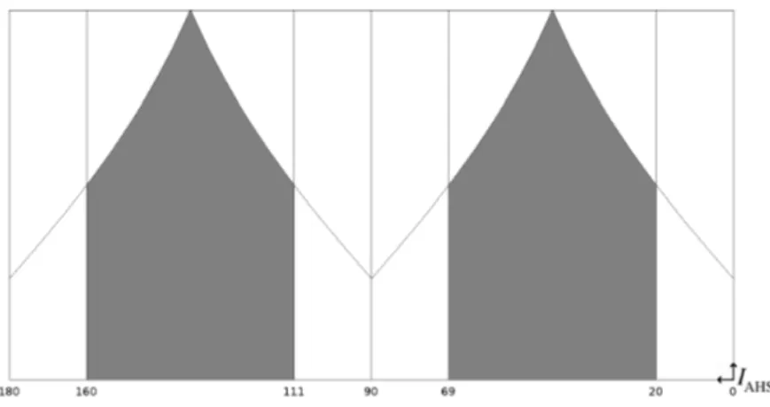
For the interval of θ ∈ [20°, 69°] ∪ [111°, 160°] we use ∆θ = 0.5°, which is enough for the detection and well balanced between the required computations and the quality of the results.
The value of ∆ρ can be defined using simple trigonometry. For θ ∈ [0°, 45°] the cosine function is used, and for θ ∈ [45°, 90°] the sine function.
For lines with θ < 45° we want to increase ρ such that the projected lines intersect the x axis at intervals of 1, and for lines with θ > 45° we increase ρ such that the projected lines increase by 1 in the intersection with the y axis. This is illustrated in Fig. 3.6, where we can see that for θ = 45° we can use either the sine or cosine. We use ∆ρ = cos θ for θ ∈ [0°, 44°] and ∆ρ = sin θ for θ ∈ [45°, 90°]. In this manner we relate the intervals of Cartesian coordinates to the intervals of polar coordinates such that no lines are repeated or missed for each angle θ.
(a) 22.5° (b) 45° (c) 67.5°
Figure 3.6: Optimising the number of lines to search using trigonometry. Each plot shows one value of θ, where ρ is also represented. (a) θ = 22.5°, (b) θ = 45°, (c) θ = 67.5°. Only the right half of the image is shown.
(a) 22.5° (b) 45° (c) 67.5°
Figure 3.7: Plots showing examples of ρmax for: (a) θ = 22.5°; (b) θ = 45° and (c)
θ = 67.5°.
As all the lines that have at least 1 point in the IP image are important, the
highest value of ρ should be the straight line that passes through the opposite corner relative to the central axis in the image, which in the right half means the point where xP= WP/2and yP= HP. Using the polar equation with the previous
point we get ρmax = WP/2 × cos θ + HP× sin θ. This is illustrated in Fig. 3.7 for 3
angles (only the right half of the image is shown).
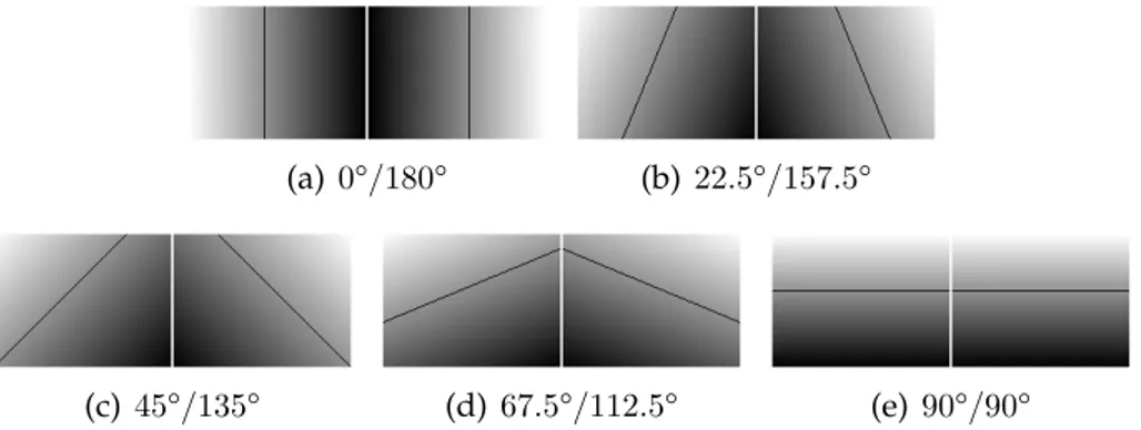
For demonstrating that no lines are skipped, Fig. 3.8 shows the projected lines in IPfor ρ ∈ [0, WP/2 × cos θ + HP× sin θ]. Each value of ρ is represented by a different
level of grey. Starting at ρ = 0, represented by black, the level of grey increases until ρ = WP/2 × cos θ + HP× sin θ represented by white. The line with value 145 (middle
(a) 0°/180° (b) 22.5°/157.5°
(c) 45°/135° (d) 67.5°/112.5° (e) 90°/90°
Figure 3.8: Examples of projected lines in IPDW for the Adapted Hough Space. Each
image represents all ρ values, and for θ: (a) 0°/180°, (b) 22.5°/157.5°, (c) 45°/135°, (d) 67.5°/112.5°, and (e) 90°/90°.
shows that no pixel was left out, as for each particular angle one and only one line was projected in the image. The left and right parts of the image are divided by a white line. Each image represents a different value of θ for the left/right halves. The values for θ in Fig. 3.8 are: (a) θ = 0°/180°; (b) θ = 22.5°/157.5°; (c) θ = 45°/135°; (d) θ = 67.5°/112.5°; (e) θ = 90°/90°.
For searching the maximum number of pixels on each projected line in IP(xP, yP),
we look for all edge pixels: (a) for θ ∈ [0°, 45°], yP= {0, 1, 2, 3, · · · , HP− 1}; (b) for
θ ∈ [45°, 90°], xP = {0, 1, 2, 3, · · · , WP/2 − 1}. This means we increment yP and
calculate xP for θ ∈ [0°, 45°], and increment xPand calculate yP for θ ∈ [45°, 90°].
Each edge pixel will be attributed to the line which has the minimum distance to its centre. This is further explained below. Examples are shown in Fig. 3.9, in which each plot represents one value of θ and several values of ρ. The values of θ represented in the figure only cover the interval θ ∈ [0°, 90°]; the lines projected at the remaining angles [90°, 180°] are symmetrical as explained later.
We restrict the Hough space to θ ∈ [20°, 69°] ∪ [111°, 160°] such that vertical and almost vertical lines in the intervals θ ∈ [0°, 20°] ∪ [160°, 180°] are ignored. The same is done for horizontal and almost horizontal lines in the interval θ ∈ [70°, 110°]. This yields a reduction of the CPU time of about 30%, and border detection is not affected since important lines are not represented in these intervals. Figure 3.10 shows the restricted Hough space. The grey part is where we will look for the
(a) 0° (b) 22.5° (c) 45° (d) 67.5° (e) 90°
Figure 3.9: Examples of line sampling. Each plot represents one value of θ: (a) 0°; (b) 22.5°; (c) 45°; (d) 67.5°; (e) 90°.
projected borders. As ∆ρ is not a static value as explained before, the vertical axis of IAHS is not ρ but ρint in order to accommodate all the values. This is related to
ρas ρint = ρ/cos(θ)for θ ∈ [0°, 44°] and ρint = ρ/sin(θ)for θ ∈ [45°, 90°] (this is for
illustration purposes only). The horizontal axis represents θ.
As we want to further optimise the computations needed to process the Hough transform, and since we have “mirrored” lines (about the y axis) for θ and π − θ for the same values of ρ, we only calculate the lines for θ ∈ [0°, 90°]. The right border we denote by Lρ,θ(xP,r, yP). Similarly, the lines for θ ∈ [91°, 180°] are computed for
the left border, Lρ,π−θ(xP,l, yP), because of the mirrored lines.
For Lρ,θwe use xP,r = (ρ − yPsin θ)/ cos θand yP= (ρ − xP,rcos θ)/ sin θ, and for
Lρ,π−θwe use xP,l = −xP,r− 1 and the same yPbecause of the mirroring. This way
we do not need to calculate all the points again for the left borders; we only need to invert the signal of the x value. This yields a reduction of CPU time of about 50%, as we need a little more than half of all computations.
This means that IAHS(0, 0°) corresponds to a vertical line with yP = [0, HP− 1]
and xP,r = 0, and that IAHS(0, 180°) has the same yP but xP,l = −1. For obtaining
the maximum number of pixels on the projected lines Lρ,θ and Lρ,π−θ, we increment
by 1 the yP and compute the corresponding xP,r and xP,l for θ ∈ [0°, 44°]. For
θ ∈ [45°, 89°] we increment by 1 the xP,r, with xP,l = −xP,r− 1, and calculate the
corresponding yP.
The image IAHS(ρ, θ) has the origin at the bottom-right corner because of the
Figure 3.10: The restricted AHS. The grey areas will be analysed for detecting path borders.
represented on the left and right parts of IAHS.
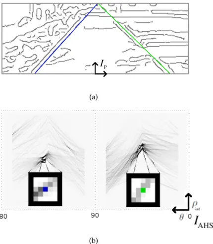
An example of the IAHS, together with the corresponding IP, is shown in Fig. 3.11,
respectively (a) and (b). The left border is marked in blue in both images, as the right border in green.
The IAHSspace is filled by checking the pixels in IPfrom top to bottom:
left-to-right for the left-to-right border (Lρ,θ)and right-to-left for the left border (Lρ,π−θ). As for the
normal Hough space, IAHSis a histogram which is used to count the co-occurrences
of aligned pixels in the binary edge map IP.
However, longer sequences of edge pixels count more than short sequences or not-connected edge-pixels. To this purpose we use a counter P which can be increased or reset. When we check each pixel in IP for a projected line Lρ,θ and
find the 1st ON pixel, P = 1 and the corresponding IAHS(ρ, θ) = 1. If the 2nd pixel
following the first ON pixel is also ON, P will be incremented by 2, and IAHS(ρ, θ)is
incremented by P = 3 so IAHS = 4. For the 3rd connected pixel P = 5, and IAHS= 9,
and so on (the values are only for a first sequence of ON pixels). If a next pixel is OFF, the variable P is reset to 0 and IAHS(ρ, θ)is not changed. In other words, a run
of n connected edge pixels has P values of 1, 3, 5, 7, etc., or Pn = Pn−1+ 2, with
P1 = 1, and the run will contribute n2 to the relevant IAHSbin. For each line, a pixel
is considered ON if the pixel at the calculated position is ON, or if: (a) for lines at θ ∈ [0°, 44°] the pixel to the left or to the right of the calculated position is ON; (b)
(a)
(b)
Figure 3.11: (a) IP with detected borders in colour; (b) Corresponding IAHS with
magnified regions around the detected borders. The left and right borders are marked in both in blue and green, respectively.
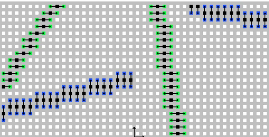
for lines at θ ∈ [45°, 90°] the upper or the lower pixel is ON. Four examples of lines are shown in Fig. 3.12, two for each side, one in green (θ ∈ [0°, 44°]) and one in blue (θ ∈ [45°, 90°]). The calculated lines are shown in black.
The final value of an IAHS(ρ, θ)bin is the sum of the Pnvalue(s) of all sequences
of ON pixel(s): IAHS(ρ, θ) =
Pk
l=1Pn,l with k the number of sequence(s) of ON
pixel(s) and each sequence having at least one ON pixel. Figure 3.11(a) shows an example, with the left and right borders superimposed. The corresponding IAHSis
Figure 3.12: AHS line checking example.
and right borders are marked in blue and green, respectively, also in the edge map IPin Fig. 3.11(a).
Until here we explained the computation of IAHS, but only during the
initiali-sation phase, i.e., the first 5 frames. After the initialiinitiali-sation phase, for optimiinitiali-sation and accuracy purposes, we will not check the entire IAHSspace. Each left and right
border is stored during the initialisation in array Mi(ρ, θ), with i the frame number.
After the fifth frame (i = 6), we already have five pairs of points in M , which define two regions in IAHS. These regions indicate where in IAHS,ithe next border positions
are expected. The regions are limited by the minima ρmin,l/rand θmin,l/r, and by the
maxima ρmax,l/rand θmax,l/r, in the left and the right halves of IAHS. In frames i ≥ 6,
we look for the highest value(s) in IAHS,i(ρ, θ)in the regions between ρmin,l/r− Tρ
and ρmax,l/r+ Tρ, and between θmin,l/r− Tθand θmax,l/r+ Tθ, on the left and on the
right side respectively, with Tρ = 10 × ∆ρ and Tθ = 10 × ∆θ. This procedure is
applied for all i ≥ 6, always considering the borders found in the previous five frames. An example is shown in Fig. 3.13, where the brighter grey area represents the space restriction during initialisation. The darker grey represents an example of the restriction after initialisation, with the white points inside this region being the 5 previously detected borders.
For selecting the path borders we analyse the successive highest values of IAHS
Figure 3.13: An example of the restriction of the Adapted Hough Space during and after the initialisation stage. The dark grey area is where lines are searched after the initialisation, and brighter grey during initialisation. Also marked in white the points that determine the restricted region, respectively the detected borders for each side for the last 5 frames.
intersection point, the VP. If the intersection point of the next left and/or right value(s) has a smaller Euclidian distance to the VP of the previous frame, we still continue checking the next highest value(s) on the corresponding side(s). If this does not yield an intersection point with a smaller Euclidian distance to the VP, the current value is selected. After both values have been selected, their intersection corresponds to the new frame’s VP. In this search, all combinations of left and right border candidates are considered. After the initialisation, if in the left or right regions where the IAHSvalues are checked there is no maximum which corresponds
to at least one sequence of not less than 10 connected ON pixels, IAHSis checked
again but without region restrictions, i.e., the procedure during initialisation, as in Fig. 3.10, is applied. If still no correspondence can be found, the border is considered not found for that side. In this case, the average of the last 5 borders found is used. If after 5 consecutive frames one or both borders are not found, the user is warned. The HL value remains the same, and the scanned window expands to the left-and/or rightmost column according to the missing border(s). Delimited by the detected borders is the walkable path, called the Path Window (PW) as explained next.
3.5
Path window (PW)
As we only want to process the walkable path area for detecting obstacles, i.e., where the user can walk, the next step is to create an image which only contains this area. We call this the Path Window (PW). It comprises the area limited by the left and right borders, below the HL (or VP where the borders intersect).
The new image IPW will have the axes positioned as in the previous IPDW.
It is then defined as IPW(xPW, yPW), and is delimited by the L1L (left limit), L1R
(right limit) and yPW = 0. These borders are shown later in Fig. 4.3. Calculated
previously in Chap. 3.4, we will use these lines to define the PW. However, we have to scale them back, as they are obtained from the re-scaled image IP. Using polar
coordinates, we can use the angle of the previously calculated border in IP, as the
scaling does not affect the angle. So, θPDW = θP. Concerting distance to the centre,
this will be scaled according to the scaling factor S = WPDW/WP= HPDW/HPused
in IP, where ρPDW = ρP× S.
An example is shown in Fig. 3.14. The PW is delimited by a black line, inside the previous size of the original image indicated by a dashed line.
(a) (b)
Figure 3.14: (a) Original image with detected path; (b) The path window PW is the triangular area.
Chapter 4
Obstacle detection
4.1
Introduction
The detection of obstacles is explained in this chapter. Common processing that precedes the detection algorithms is explained first in Section 4.2, with the creation of the obstacle detection window. Section 4.2.1 is about the window size used for obstacle detection, and 4.2.2 is about the method of “squaring” the resulting image for correction perspective projection. In Section 4.2.3 common pre-processing of the obstacle detection window is described. Then, three obstacle detection algorithms are detailed in Sections 4.3, 4.4 and 4.5: Zero crossing counting, Histograms of binary edges, and Laws’ texture masks. Finally, we conclude this chapter with the avoidance of a detected obstacle in Section 4.6.
4.2
Obstacle detection window (ODW)
We start by using the previously detected path window PW, narrow it to the obstacle window OW, and then resize it to the obstacle detection window ODW with correction of the perspective projection. These steps are illustrated in Fig. 4.1.
(a) PW (b) OW (c) ODW
Figure 4.1: Creating the obstacle detection window. Starting with (a) the PW, we then create (b) the OW, and finally (c) the ODW with correction of perspective projection.
4.2.1
Window size
We have to consider a minimum and a maximum distance in front of the user for obstacle detection. The first meter is in reach of the white cane. Even if a user walks at a pace of 1 m/s (more than average), and there is an obstacle at 8 meters distance, he still has approximately 7 seconds until the obstacle is in reach of the white cane. During this time the user can be alerted to the obstacle at a reasonable distance, with at least 5 seconds until reaching it. Distances as measured in the input image depend on the used camera.
With the camera in use, which we previously presented, an image was captured of several lines with 1 meter intervals. The camera was aligned vertically at 1.5 meters from the ground. This image is shown in Fig. 4.2. The bottom line of the image is at a distance of 2.5 meter from the camera. The lines in the image with 1 meter spacing on the ground range from 3 to 8 meters. This means that the examples shown are for obstacle detection approximately in the range of 2.5 to 8 meters distance from the user. The same camera was used to capture the images in Chap. 5, where we show results. Different cameras, and especially different lenses, will have different ranges in depth. Therefore each camera should be calibrated. The only requirement is that the range for detection should be enough such that, after the obstacle is detected, the user can be instructed in time about the best way to avoid it, while at a distance of 3 to 5 meters.
Figure 4.2: Distance calibration for obstacle detection.
At this point we must stress that our system will not detect obstacles at a distance of less than 2 m from the user, because of two reasons: (i) The user has already been alerted to a looming obstacle at a larger distance and advised to adapt path trajectory: (ii) The user will always check a detected obstacle using the white cane at short distance.
The PW previously detected (IPW) may still contain part of the borders of the
sidewalk, so we can ignore a part on each side of the PW. This is done relative to the VP. A line drawn on each side (left/right), defined by the VP and a point on the bottom line of IPW, yields a smaller window IOW, or Obstacle Window (OW), with
coordinates as in IPW.
The point at bottom line of the image and the left border (L1L), we call P1L; that
of the right border (L1R) we call P1R; see Fig. 4.3. We have to stress that P1Lis never
Figure 4.3: PW with reference points and lines marked in blue and green respectively to determine the OW.
and P1R= WIN/2−1. Lines L1Land L1Rmay not correspond to the real path borders,
if the latter intersects the left or right image borders. If this happens, lines L1L and
L1Rwill be used to limit the size and reduce the computations needed.
Points P2Land P2Rare located ×5% of WPWto the right and to the left from the
points P1Land P1R, as shown in Fig. 4.3.
The height of IOW is determined by the VP’s vertical position, as HOW =
(2/3)yVP, and so are the points P3L and P3Rwhich are the intersections between line
y = (2/3)yVP and the lines between points P2L and P2R.
The OW limits will be the lines between points P2Land P3L, for the left limit L2L,
and between P2Rand P3R, for the right limit L2R.
(a) (b)
Figure 4.4: (a) the original image with the reduced OW; (b) the OW image with the limits marked in black. The limits marked in grey are from the PW, and the dashed limits the original image.
4.2.2
Correction of perspective projection
As all detection algorithms are based on an analysis of the lines and columns separately, it is more efficient to convert the trapezoidal window into a rectangular one. Due to perspective projection, the window resulting from path detection has more detail at the bottom than at the top. As we prefer a rectangular image, and to have more homogeneous detail in depth, a correction is applied. The resulting image we will call obstacle detection window (ODW), in which we will look for obstacles.
The correction is based on mapping the trapezoidal window to a rectangular one, as illustrated in Fig. 4.5. The width of the rectangular window corresponds to the width of the reduced OW at y = (2/3)yVP, and the height equals (2/3)yVP.
Hence, the top line of the rectangular window equals the top line of the reduced OW. The other pixels of the rectangular window are computed by (a) drawing projection lines through the VP and the pixels on the top line, and (b) using linear interpolation of the pixels on the non-top lines along the drawn projection lines. As a result, the resolution at the top line will be preserved, but at the bottom line it will be decreased. However, most obstacle will be detected near the top line, where
(a) (b)
Figure 4.5: Correction of perspective projection: (a) the principle, original (top) and corrected (bottom); (b) shows a real example, the original OW (top) and the corrected image (bottom).
image resolution was already lower. After correction, image resolution is more homogeneous.
The previously shown image in Fig. 4.4(b) is used in Fig. 4.5(b) as a real example, before correction (top) and after correction (bottom). One can notice less detail in the lower part.
4.2.3
Image pre-processing
After the ODW has been determined as explained before, a pre-processing is applied to remove image “noise” and to reduce the computation time.
In Fig. 4.6 the image used for demonstrating this pre-processing is shown, in (a) the original grayscale image, and in (b) with the OW highlighted. Figure 4.7(a) shows the ODW to which the pre-processing is applied.
(a) (b)
Figure 4.6: Test image used for obstacle detection: (a) original in grayscale; (b) OW highlighted.
After the correction of perspective projection, the ODW is resized to half the height and width using again bilinear interpolation. We then apply a Gaussian low-pass filter with a 3 × 3 kernel. This results in the pre-processed image to which we still call IODW. This pre-processing is common to all obstacle detection algorithms,
as we use the same input image for each. From now on, IODWrefers to the image
after pre-processing.
An example is shown in Fig. 4.7, with (a) the original ODW image and (b) the ODW after the pre-processing as explained. Although reduced in size, the latter is shown at double size for comparison purpose.
4.3
Zero crossing counting algorithm
This algorithm is based on the idea that obstacles usually have some contrast with the path texture (ground). It is inspired by [8], but with considerable modifications.
First x and y derivatives are applied to the IODW image, as explained in
Sec-tion 4.3.1. Thresholds are applied to the derivatives in order to remove noise resulting from the ground texture, which is shown in Section 4.3.3. The obstacle region can be obtained by computing the histograms of the x and y zero
cross-(a) (b)
Figure 4.7: (a) the ODW image. (b) the ODW image after resizing (shown here at the same size, although the resolution difference can be noticed) and low-pass filtering. ings (Section 4.3.2) and by projecting the histograms into the ODW, where another threshold is used to avoid false obstacles (Section 4.3.3).
4.3.1
Horizontal and vertical first derivative
We will process the x and y derivatives using a large kernel for increasing the differ-ence between regions with similar pixels and regions with very different pixel inten-sities. For the derivatives we use the kernel K = h−1 −1 −1 0 +1 +1 +1i. The x derivative image is called IODW,dxand is shown in Fig. 4.8(a). The y derivative
image is called IODW,dyand shown in Fig. 4.8(b).
4.3.2
Zero crossing counting
After computing the derivatives we sum the amplitudes of the maximum and minimum values near every zero-crossing (ZC). By this we mean that every time the pixel value crosses zero, we search for the minimum and maximum value on
(a) (b)
Figure 4.8: Derivatives applied to the image in Fig. 4.7(b): (a) dx; (b) dy. each side and sum the absolute values. These values are then summed over lines (x derivative) and over columns (y derivative).
For storing the variation over all lines, we use the array SZC,dx(y) for the x
derivative (IODW,dx), where y ∈ [0, HODW,dx− 1] (the number of lines in the image).
Similarly, to check the variation over all columns, we use the array SZC,dy(x)for
the y derivative (IODW,dy), where x ∈ [0, WODW,dy− 1] (the number of columns in the
image).
Array SZC,dxis filled by analysing every line in the image, and SZC,dyby analysing
every column. After this, these arrays are smoothed two times with a 7 × 1 kernel. Figure 4.9(a) shows an example of the x derivative, with the smoothed SZC,dx
values overlaid on the left. Figure 4.9(b) shows the same in case of SZC,dy (y
deriva-tive).
4.3.3
Thresholding and final region detection
The two histogram arrays must be thresholded in order to improve the detection of the region where an obstacle may be present. During system initialisation, the
first 5 frames are supposed to have no obstacle and the two thresholds are updated using the maximum and minimum values of the derivatives. Hence, the thresholds can adapt to the type of the pavement, i.e., we can remove the “noise” caused by the ground texture. After the initial 5 frames, the thresholds are also updated using the maximum and minimum values, but only in the bottom part of the image, the part nearest to the user. While the user walks forward, an obstacle can be present first in the top part of the image, and when the user approaches the obstacle it tends to go to the bottom of the image. We consider the lower half of the ODW image for updating the thresholds.
Let TM ax/M in,dx/dy denote the maximum/minimum thresholds of the x/y
deriva-tives. All derivative values in the interval [TM in,dx/dy, TM ax,dx/dy]will be set to zero in
the derivative images dx/dy. It should be stressed that this is done before counting the zero crossings as explained in Section 4.3.2.
Consider i to be the frame number of the sequence. In the initial 5 frames (1 ≥ i ≥ 5), TM ax,dx/dy are set to the maximum values of IODW,dx/dy(x, y), and
TM in,dx/dy to the minimum values, considering the values in the entire 5 images:
x ∈ [−WODW/2, WODW/2 − 1] and y ∈ [0, HODW − 1]. After initialisation (i ≥ 6)
the thresholds are updated using the bottom half: y ∈ [0, HODW/2 − 1]. If a new
threshold is higher or lower (according to the maximum or the minimum) than the previous one (i − 1), the threshold is set to the new one. If it is lower than the maximum or higher than the minimum, the threshold is updated using the average between the new and the old values, TM ax/M in,i = (max/mini+ max/mini−1)/2.
The above procedures serve to adapt the thresholds of the x and y derivatives before filling the x and y histograms. After filling the histograms for each new frame i, we can detect the obstacles region.
For selecting the region where the obstacle can be we look for the “intersection” of the histograms in SZC,dx(y), with y ∈ [0, HODW − 1] and in SZC,dy(x), with
x ∈ [0, WODW− 1].
Yet another threshold is applied to both SZC,dx/dy: all values below 3 are ignored
to remove noise caused by the ground texture.
(a) (b) (c) (d)
Figure 4.9: The derivatives dx and dy: (a) dx, at the left the ZC histogram; (b) dy, at the bottom the ZC histogram. (c) the multiplication of the thresholded histograms; (d) the detected region overlaid on the obstacle detection window.
of the corresponding histograms SZC,dx and SZC,dy. In words, the histograms are
back-projected into the ODW and their intersection is computed.
Figure 4.9 shows examples of the histograms (a) and (b), the region in (c) and in the original in (d).
4.4
Histograms of binary edges algorithm
The Canny edge detector [33] is applied to the IODW image. This results in the
first derivatives dx and dy, the corresponding edge magnitude represented in IC,mag(x, y) = pdx(x, y)2+ dy(x, y)2, and the corresponding edge orientation in
IC,θ(x, y) = arctan (dy(x, y)/dx(x, y)). The Canny algorithm is applied with σ = 1.0,
which defines the size of the Gaussian filter, in combination with Tl= 0.25which is
the low threshold for hysteresis edge tracking. The value of the high threshold Th
is explained in Section 4.4.2. The final result is a binary edge map ICas shown in
(a) (b) (c) (d)
Figure 4.10: Starting with the orientation division for selecting horizontal, vertical and common edges (a), then the binary edge image (b), which is split into horizontal and vertical edges, respectively IC,Hin (c) and IC,V in (d).
4.4.1
Horizontal and vertical edges
As we want to determine the region where the obstacle is, we split IC according
to the derivatives’ orientations. The orientation angles are divided into 8 inter-vals: for horizontal edges θH ∈ [−3π/8, 3π/8] ∪ [5π/8, −5π/8]; for vertical ones
θV ∈ [π/8, 7π/8] ∪ [−7π/8, −π/8]. Horizontal and vertical edges are stored in
the images IC,H and IC,V. In 4 common intervals (where the previous overlap),
some edges may be both vertical and horizontal, which is normally at corners, so these are preserved in both images. This division is shown in Fig. 4.10(a), with the main intervals indicated by horizontal or vertical lines, and the common intervals hatched.
Figure 4.10 shows the orientation division for selecting horizontal, vertical and common edges in (a), the original Canny edge map in (b), the horizontal edges in (c), and the vertical edges in (d).
4.4.2
Thresholding and final result
To compute dynamically the high threshold Th, we use IODW,mag, the magnitude
(a) (b) (c) (d)
Figure 4.11: Binary edge images with histograms in grey: (a) IC,H; (b) IC,V. The
detected region is shown in (c), also in (d) overlaid in the original.
of the sequence. During initialisation, i ≤ 5, the overall maximum value is used: Th = maxi[IODW,mag]. For i ≥ 6, if the maximum in the bottom half of IODW,mag(x, y),
with x ∈ [−WODW/2, WODW/2 − 1] and y ∈ [0, HODW/2 − 1], is higher than the
threshold of the previous frame (maxi > Th,i−1), then Th,i = maxi; otherwise
Th,i = (maxi+ Th,i−1)/2. As in Section 4.3.3, this allows the algorithm to adapt to
different types of pavements.
For finding the region where the obstacle may be, histograms of lines and columns are calculated using IC,H and IC,V. In IC,H, the columns are summed. The
same is applied to IC,V, where the lines are summed. This is denoted by SC,H(x)for
the IC,H histogram, and SC,V(y)for the IC,Vhistogram, with x ∈ [0, WODW− 1] and
y ∈ [0, HODW− 1].
A threshold is applied to both histograms SC,H and SC,V. All values below 2 are
ignored, because we only consider an obstacle detected if at least 2 entries in the same line/column are found. The image IHC(x, y)is the result of the multiplication
(back-projection) of the SC,H(x)and SC,V(y)histograms. In Fig. 4.11, the thresholded
histograms are shown, in (a) for columns (horizontal edges), and in (b) for lines (vertical edges), as well as the result from histogram multiplication for region finding in (c), and the latter overlaid in the original image in (d).
4.5
Laws’ texture masks algorithm
The third algorithm is based on Laws’ texture energy masks [35] applied to IODW.
The main idea is to detect changes in the image textures. If the frames contain textures before an obstacle enters the ODW, these will not be detected through the use of a threshold value.
Laws’ masks result from the 2D convolution of the kernels for edges (E), smooth-ing (L), spots (S), wave (W) and ripples (R): E5 = [-1 -2 0 2 1]; L5 = [1 4 6 4 1]; S5 = [-1 0 2 0 -1]; W5 = [-1 2 0 -2 1]; R5 = [1 -4 6 -4 1].
As in [35], previous tests showed that the best masks for extracting texture features are E5L5, R5R5, E5S5 and L5S5, which result from the 2D convolution of the 1D kernels listed above. These masks are shown in Fig. 4.12.
-1 -4 -6 -4 -1 -2 -8 -12 -8 -2 0 0 0 0 0 2 8 12 8 2 1 4 6 4 1 (a) E5L5 1 -4 6 -4 1 -4 16 -24 16 -4 6 -24 36 -24 6 -4 16 -24 16 -4 1 -4 6 -4 1 (b) R5R5 -1 0 2 0 -1 -2 0 4 0 -2 0 0 0 0 0 2 0 -4 0 2 1 0 -2 0 1 (c) E5S5 -1 0 2 0 -1 -4 0 8 0 -4 -6 0 12 0 -6 -4 0 8 0 -4 -1 0 2 0 -1 (d) L5S5
Figure 4.12: Laws’ masks: (a) E5L5; (b) R5R5; (c) E5S5; (d) L5S5.
4.5.1
Laws’ masks feature extraction
After filtering with the masks, an energy measure Elm(x, y) =
P5
i,j=−5IODW,lm(x +
i, y + j)2of size 11x11 is applied to the neighbourhood of each point in the IODW,lm
image, where lm represents each of the four Laws’ masks. The four energy images are then normalised using the maximal energy responses that each mask can have,
such that each mask contributes equally to final detection. These maximal energy responses are: (a) E5L5 48C; (b) R5R5 128C; (c) E5S5 12C; and (d) L5S5 32C. The value C corresponds to the maximum level of grey; here we use 256 levels of grey, from 0 to 255.
It can be seen in Fig. 4.13(b) and (c), that masks R5R5 and E5S5 do not respond to this type of pavement/object. This is normal, as the four masks are chosen to distinguish between different textures.
The four normalised energy images are then summed and the result is nor-malised again as shown in Fig. 4.14(a).
(a) E5L5 (b) R5R5 (c) E5S5 (d) L5S5
Figure 4.13: Laws’ masks algorithm results: (a) E5L5; (b) R5R5; (c) E5S5; (d) L5S5. Results in (b) and (c) are zero, which is due to the particular image texture, but these masks can have non-zero responses in case of other images.
4.5.2
Thresholding and final result
All values above 4% of the maximum value are considered to be due to a possible obstacle. The remaining dynamic thesholding process is similar to the one in the zero crossing counting algorithm (Section 4.3.3).
If TM ax,lmdenotes the maximum threshold of each mask, we set all values below
this threshold to zero. If i is the frame number of the sequence, during initiali-sation (1 ≥ i ≥ 5) TM ax,lm will be set to the maximum values in the IODW,lm(x, y),
(a) Sum (b) Region (c) Overlaid
Figure 4.14: The summed result of the Laws’ masks is shown in (a), which results in the region shown in (b), and overlaid in the ODW image in (c).
and they are updated using the maximum values of the entire five ODW images: x ∈ [0, WODW − 1] and y ∈ [0, HODW − 1] in each image. After initialisation
(i ≥ 6) the thresholds are updated using the lower half of the ODW image, where x ∈ [−WODW/2, WODW/2 − 1]and y ∈ [0, HODW/2 − 1]. If the new threshold is
higher than the previous one (i − 1), the threshold is set to the new one. If it is lower, the threshold is updated with the average between the new and the old values, Tmax,i = (maxi+ maxi−1)/2.
Results are shown in Fig. 4.14: (a) summed, (b) thresholded, and (c) the resulting region overlaid in the original.
4.6
Obstacle avoidance
If an obstacle is detected (a) in at least 3 consecutive frames, (b) by at least two of the three algorithms in each frame, and (c) with obstacle regions in the ODW whose intersections are not empty, the user will be alerted. In addition, in order to avoid the obstacle, the user is instructed to turn a bit left or right. This is done by comparing the obstacle’s region with the open spaces to the left and right in the path window. This is shown in Fig. 4.15, where in this case the distances from the
obstacle to the path borders are similar, so the system can choose which side to go.
Figure 4.15: Obstacle avoidance decision
Hence, the user can adapt his route when approaching the obstacle, in the ideal case turning a bit until the obstacle is not any more on his path. It should be stressed again that the user will always use the white cane in order to check the space immediately in front. In addition, the user should check and confirm an obstacle after being alerted, because there may be false positives but also false negatives in obstacle detection. This is subject to further research. Still under development is the interaction between obstacle avoidance and correct centering on the path, such that avoidance does not lead to leaving the path.
Chapter 5
Results
In this chapter we show and discuss results of applying the algorithms, both for path and for obstacle detection. First we present two images with detailed results, and later several sequences in which path detection as well as obstacle detection is shown.
The original image is always shown, overlayed with the path limits and the obstacle detection window, in which obstacles, if they exist, are highlighted. The left and right limits are the ones nearest to the borders of the path, which intersect at a point near the centre of the image. The obstacle detection window is located in the lower part of the image, delimited by the previously described limits. Inside this window, obstacles will be highlighted using two different levels of grey: the lighter means a higher probability of an obstacle being present (detected by all three algorithms), and the darker means a lower probability, although still considered an obstacle (detected by two of the three algorithms).
The first result summarises the previously presented example, where a trash bin is in the centre of a corridor. The top row in Fig. 5.1 shows the original image and the same image with the path detected, and the detected obstacle. The bottom row shows, from left, the obstacle detection window as input for the obstacle detection algorithms; the x derivative with the histogram at the left; the y derivative with the histogram at the bottom; the result from the 1st obstacle detection algorithm (Zero