Faculdade de Ciências e Tecnologia
Universidade do Algarve
Settlement patterns of mussel recruits at different
temporal scales in the Peniche-Berlengas area
(Southwest Portugal).
Joana Pimentel Santos da Conceição
Dissertation for Master’s degree in Marine Biology
Supervisors: Doutora Laura Peteiro, University of Aveiro
Prof. Doutora Alexandra Chícharo
,
University of Algarve.2 Settlement patterns of mussel recruits at different temporal scales in the Peniche-Berlengas area (Southeast Portugal).
Declaração de autoria do trabalho:
Declaro ser a autora deste trabalho, que é original e inédito. Autores e trabalhos consultados estão devidamente citados no texto e constam da listagem de referências incluída.
____________________________________________________
Copyright
A Universidade do Algarve tem o direito, perpétuo e sem limites geográficos, de arquivar e publicitar este trabalho através de exemplares impressos reproduzidos em papel ou de forma digital, ou por qualquer outro meio conhecido ou que venha a ser inventado, de o divulgar através de repositórios científicos e de admitir a sua cópia e distribuição com objetivos educacionais ou de investigação, não comerciais, desde que seja dado crédito ao autor e editor.
3
Institutions
This master thesis is inserted in the project “LarvalSources – Assessing the ecological performance of marine protected area (MPA) networks” funded by the FCT (PTDC/BIA-BIC/120483/2010). All the lab and writing work will be performed in Department of Biology at University of Aveiro, while the field work will be carried out in Berlengas Natural Reserve, Peniche and neighborhood, with the necessary help and support of ICNF (Instituto da Conservação da Natureza e das Florestas) and Escola Superior de Turismo e Tecnologia do Mar de Peniche (ESTM-IPL, Peniche).
4
Acknowledgments
To all my laboratory colleagues I would like to thank, especially to Laura, Inês and Rui who tirelessly accompanied me and helped throughout the fieldwork. I would like to leave a special thanks to Laura for being by my side during the entire work. To Professor Henrique Queiroga for giving me the opportunity to undertake this study. To all my MSc’ classmates that even with its own ongoing projects were always concerned with each other’s. And finally, to my fabulous parents, and to Allan who were always willing to help.
“Façam o favor de ser felizes..!”
5
Table of
Contents
Resumo ... 10 Abstract ... 11 Theme Choice ... 12 Literature review ... 14Marine Protected Areas ... 14
Mytilus galloprovincialis, as a model species. ... 15
Objectives ... 22
Methodology ... 23
Surveys and sampling sites ... 23
Data analysis ... 25
Results ... 29
Environmental parameters ... 29
Settlement time series (monthly sampling)... 40
Settlement time series (spring sampling – every other day) ... 46
Histograms, cohort analysis and growth rate ... 51
Discussion and Conclusions ... 61
6
Figures Index
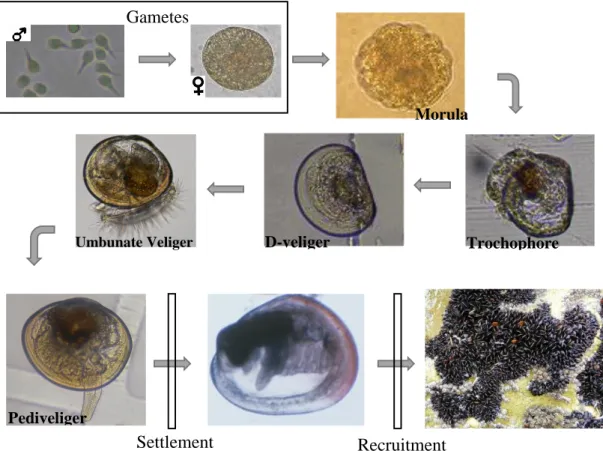
Figure 1 - Mytilus galloprovincialis life cycle. Photographs by Cristina Rodríguez. 16 Figure 2 - Processes influencing dynamics population of coastal species with
planktonic larval stages. Adapted from Pineda (2000). ... 17
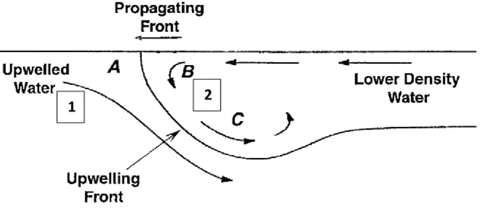
Figure 3 – Illustration of the water movements within an upwelling front
propagating shoreward. A, B and C are larval concentration points depending on their initial position and migration capacities. Strong swimmers larvae with near-surface preferences can overcome the flow and become concentrated in A or B depending on their origin. In the other hand, if the larvae have weak swimming capabilities or slow behavioural response, they will be carried down with the flow before going up again and concentrate at C. Adapted from (Shanks et al. 2000). ... 19
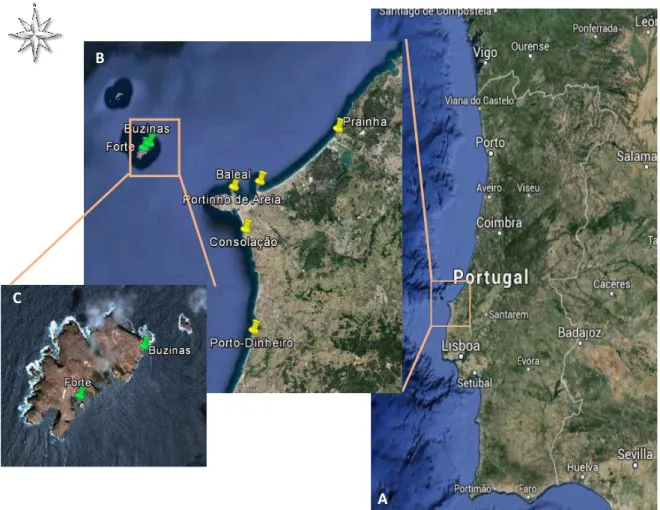
Figure 4 - Sampling sites in area of Peniche. (C) Berlengas Natural Reserve: Buzinas
and Forte; (B) Neighbouring area of the reserve: Foz do Arelho (Prainha), Baleal, Casa (Portinho de Areia), Consolação e Porto-Dinheiro. ... 24
Figure 5 – Collecting natural substrate samples (A) and artificial collectors
(scouring pads) (B). ... 25
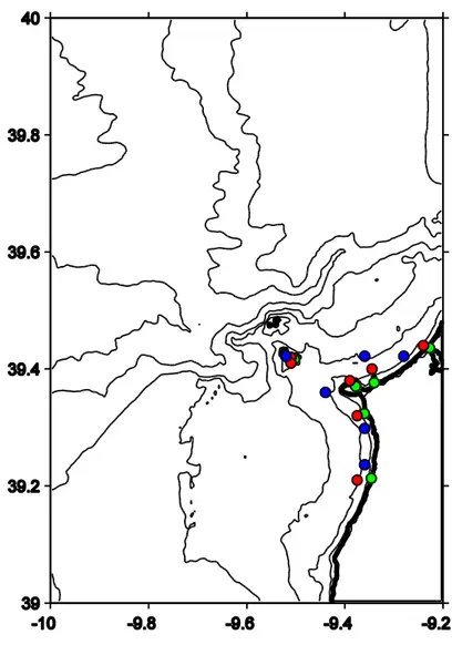
Figure 6 – Position of the collection points of environmental data (chl-a – green;
temperature and salinity – blue), in relation to the sampling sites (red). ... 26
Figure 7 - Evolution of temperature during the sampling months in the different
sampling locations. ... 29
Figure 8 - Result of the Generalized Additive Models (GAM), showing the partial
effect of Day of the Year on Temperature. Dotted lines indicate 95% confidence intervals, and tick marks along the X-axis below each curve represent effect values where observations occurred. ... 30 Figure 9 - Evolution of salinity during the sampling months in the different sampling locations. ... 31
Figure 10 - Result of the Generalized Additive Models (GAM), showing the partial
effect of Day of the Year on Salinity. Dotted lines indicate 95% confidence intervals, and tick marks along the X-axis below each curve represent effect values where observations occurred. ... 32
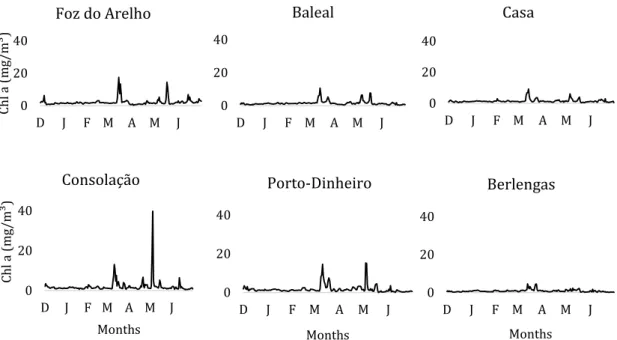
Figure 11 - Evolution of Chl a concentration (mg/m³) during the sampling months
in the different sampling locations. ... 33
Figure 12 - Result of the Generalized Additive Models (GAM), showing the partial
7 confidence intervals, and tick marks along the X-axis below each curve represent effect values where observations occurred. ... 34
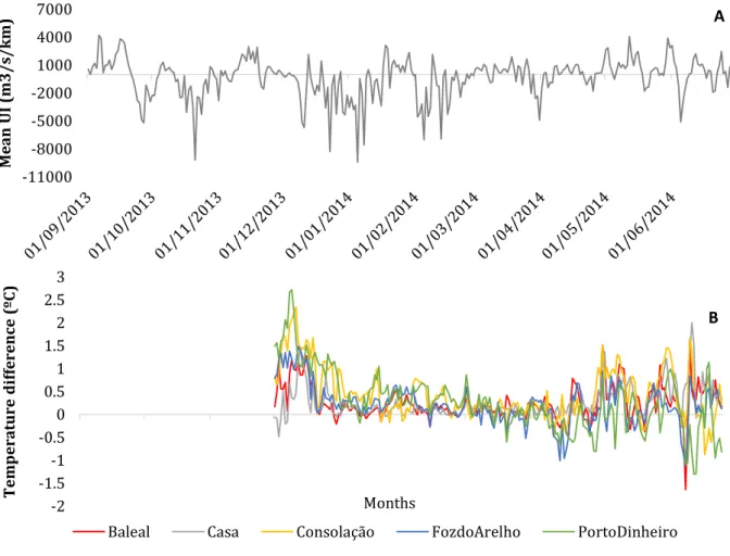
Figure 13 - At the top (A) is represented the upwelling index (m3/s/km) from September 2013 to June 2014, while in the bottom (B) is the temperature difference (temperature of Berlengas minus the temperature of each mainland location - ºC), along the sampling months. ... 35
Figure 14 - Result of the Generalized Additive Models (GAM), showing the partial
effect of Upwelling Index averaged during the last 5 and 10 days (m3 s-1 km-1) in the temperature difference (ºC) at each mainland location (from top to bottom, in the same way as from North to South: A) Foz do Arelho, B) Baleal, C) Casa, D) Consolação, E) Porto-Dinheiro). Dotted lines indicate 95% confidence intervals, and tick marks along the X-axis below each curve represent effect values where observations occurred. ... 39
Figure 15 - Settlement time series, with the number of individuals with less than
0.600 mm per sampled area (36cm²), between December 2013 and June 2014, in every sampling location. On the left are represented Buzinas, Forte, Baleal, Casa, Consolação and Porto-Dinheiro. On the right is only Foz do Arelho, with a totally different scale. ... 40
Figure 16 - Scaled abundance of the early settlers (<0.6 mm) in every locations,
between December 2013 and June 2014. Locations: left to right, corresponds to North to South. ... 42
Figure 17- Settlement time series, with the number of individuals between 0.600
mm and 2 mm, per sampled area (36cm²), between December 2013 and June 2014, in every sampling location. On the left are represented Buzinas, Forte, Baleal, Casa, Consolação and Porto-Dinheiro. On the right is only Foz do Arelho, with a totally different scale. ... 43
Figure 18 - Scaled abundance of the plantigrades (0.6 to 2 mm) in every locations,
between December 2013 and June 2014. Locations: left to right, corresponds to North to South. ... 45
Figure 19 - Settlement time series during May (spring season) every two days in
two locations, Buzinas (inside de reserve) and Baleal (outside the reserve). ... 46
Figure 20 - Settlement time series during the spring season, every two days in May
2014, in Buzinas (left) and Baleal (right) and the evolution of the environmental parameters (UI, Chl-a, temperature and salinity) during the same period. ... 48
Figure 21 - Result of the Generalized Additive Models (GAM), showing the partial
effect of the variables UI mean of the previous 2 days (A), Chl-a concentration(B) on settlement abundance in Baleal. Dotted lines indicate 95% confidence intervals, and
8 tick marks along the X-axis below each curve represent effect values where observations occurred. ... 50
Figure 22 - Size frequency distribution of Mytilus galloprovincialis collected in Foz
do Arelho (left) and in Baleal (right) through the same period. In the x-axis is the shell length classes and y-axis is the mean frequency of mussels per sampled area. ... 52
Figure 23 - Size frequency distribution of Mytilus galloprovincialis collected in
Berlengas - Buzinas (left) and Forte (right) through the same period. In the x-axis is the shell length classes and y-axis is the mean frequency of mussels per sampled area. ... 53
Figure 24 - Size frequency distribution of Mytilus galloprovincialis collected in Casa,
Cape Carvoeiro. In the x-axis is the shell length classes and y-axis is the mean frequency of mussels per sampled area. ... 54
Figure 25 - Size frequency distribution of Mytilus galloprovincialis collected in
Consolação (left) and in Porto-Dinheiro (right) through the same period. In the x-axis is the shell length classes and y-x-axis is the mean frequency of mussels per sampled area. ... 55
Figure 26 - Mean cohort length of M. galloprovincialis in Foz do Arelho and Baleal
with indication of 11 and 9 cohorts respectively identified by FISAT II (C11; C1-C9). ... 56
Figure 27 - Mean cohort length of M. galloprovincialis in Buzinas and Forte with
indication of 11 and 6 cohorts respectively identified by FISAT II (C1-C11; C1-C6). ... 57
Figure 28 - Mean cohort length of M. galloprovincialis in Casa and Consolação with
indication of 8 cohorts in both locations identified by FISAT II (C1-C8). ... 58
Figure 29 - Mean cohort length of M. galloprovincialis Porto-Dinheiro with
9
Tables Index
Table 1 - Structure of the General Additive Model selected to describe Temperature.
S.E.: standard error; e.d.f.: estimated degrees of freedom. ...30
Table 2 – Structure of the General Additive Model selected to describe Salinity. S.E.:
standard error; e.d.f.: estimated degrees of freedom. ...32
Table 3 - Structure of the General Additive Model selected to describe the
Concentration of Chl-a. S.E.: standard error; e.d.f.: estimated degrees of freedom. 34
Table 4 - Result of the Generalized Additive Models (GAM), showing the partial
effect of Day of the Year on Upwelling Index (mean of 5 previous days - m3 s-1 km-1) in the temperature difference at each mainland location. Dotted lines indicate 95% confidence intervals, and tick marks along the X-axis below each curve represent effect values where observations occurred. ...37
Table 5 - Result of the Generalized Additive Models (GAM), showing the partial
effect of Day of the Year on Upwelling Index (mean of 10 previous days - m3 s-1 km -1) in the temperature difference at each mainland location. Dotted lines indicate 95% confidence intervals, and tick marks along the X-axis below each curve represent effect values where observations occurred. ...38
Table 6 - Structure of the General Additive Model selected to describe the Upwelling
Index (mean of 2 previous days) and Chl-a concentration in the mussel settlement each 2 days in May. S.E.: standard error; e.d.f.: estimated degrees of freedom. ...49
Table 7 - Estimated growth rate of the M. galloprovincialis populations at each
sampling station, calculated based on the progression in time of the cohorts identified by FISAT II. ...60
Table 8 - ANCOVA results testing the effect of time (log Time) and location (Loc)
10
Resumo
As Áreas Marinhas Protegidas são ferramentas de gestão e conservação, que estendem a proteção das espécies-alvo a todo o ecossistema dessa área, aumentando assim a preservação do habitat e da biodiversidade. No entanto, as políticas de proteção nem sempre se traduzem num aumento da população de uma determinada espécie. Este é o caso do mexilhão azul (Mytilus galloprovincialis) na Reserva Natural das Berlengas (Portugal), onde não se observou o aumento da população adulta com a política de proibição implementada em 1981. Os fatores que regulam a incorporação de novos indivíduos na população (recrutamento) são difíceis de isolar devido às interações complexas que atuam em diferentes escalas espaciais e temporais. O estudo dos padrões de assentamento espacial e temporal é um método indireto largamente aceite para inferir processos que ocorrem antes do assentamento. O efeito da Reserva Natural das Berlengas na dinâmica da população do mexilhão azul, M. galloprovincialis, foi descrito dentro da mesma e a diferentes distâncias da área protegida, a fim de comparar os efeitos da distância à reserva e os diferentes mecanismos de chegada de larvas e possíveis repercussões da reserva nas áreas adjacentes. Foram recolhidas séries temporais de assentamento em duas frequências diferentes, mensalmente e a cada dois dias. As amostras mensais foram utilizadas para descrever os efeitos sazonais na chegada de larvas, enquanto os efeitos das características hidrodinâmicas de maior frequência foram estudados através de uma amostragem mais intensa (de 2 em 2 dias) durante o pico da época reprodutiva (primavera). As diferenças encontradas nos dados de temperatura e concentração de Chl-a encontrados entre o arquipélago das Berlengas e principalmente as localizações mais a norte da costa perto de Peniche, junto com os resultados de assentamento de juvenis de M. galloprovincialis podem indicar a presença de uma frente de upwelling entre as ilhas e a costa continental, o que poderia explicar a falta de chegada de larvas às ilhas durante as épocas favoráveis de upwelling. Desta forma, a Reserva Natural das Berlengas tem um papel de reservatório em vez de fonte de larvas para outros locais.
Palavras-chave: Assentamento; Recrutamento; Mytilus galloprovincialis; Áreas
11
Abstract
Marine Protected Areas are management and conservation tools, which extend the protection of target species to the entire ecosystem enclosed in that area, enhancing habitat preservation and biodiversity. Nonetheless, protection policies are not always translated in an increase on certain species population size. This is the case of the blue mussel (Mytilus galloprovincialis) at the Berlengas Natural Reserve (Portugal), where adult population size has not increased with the non-take policy implemented in 1981. Factors regulating the incorporation of new individuals to the population (recruitment) are hard to isolate due to the complex interactions acting at different spatial and temporal scales. The study of spatial and temporal settlement patterns is a widely accepted indirect method for inferring pre-settlement processes because integrates different aspects involved in recruitment. The effect of Berlengas Natural Reserve on population’s dynamics of the blue mussel, M. galloprovincialis, will be described within the reserve and at different distances from the protected area, in order to compare the effects of distance to the reserve and the different larval delivery mechanisms and possible spill-over effects from the reserve to the adjacent areas. Settlement time series at two different frequencies (monthly and daily) were collected. Monthly samples were used to describe seasonal effects on larval delivery and high frequency hydrodynamic features effects were studied through a more intense sampling (every two days) during the peak of the reproductive season (spring). The differences in temperature data and concentration of Chl-a found between the Berlengas archipelago and especially the northern locations of the mainland coast near Peniche, along with the results of M. galloprovincialis juvenile settlement may indicate the presence of an upwelling front between the islands and mainland coast, which could explain the lack of larval delivery to the islands during favourable upwelling seasons. Thus, the Berlengas Natural Reserve plays a role as sink instead as a source of larvae to other locations.
Key-words: Settlement; Recruitment; Mytilus galloprovincialis; Marine Protected
12
Theme Choice
The importance of establishing marine protected areas is mostly related to biodiversity conservation, fisheries management and also as tools for researchers (Edgar et al. 2007). Marine protected areas have a specific goal to each different ecosystem, but their function is usually related to the enhancement of certain habitats or the abundance of particular target species (Halpern 2003). The influence of marine protected areas on ecological functioning of marine ecosystems can have a great variety of responses from one region to another. Depending on the complexity of processes occurring within each area, the reactions of species are very difficult to predict (Halpern 2003). MPAs can indirectly favour unprotected locations, acting as an enhanced source of adults, juvenile and larvae for sink-adjacent areas (Cudney-Bueno et al. 2009) and in some cases the expected enhancement on protected population is not directly observed (Cole et al. 2011).
About the efficacy of MPAs, it has been determined that location, size and spacing of MPAs are crucial factors on MPAs design which are going to condition their efficiency, and should be selected according to habitat requirements and meta-population dynamics of key species. Understanding of those dynamics require the development of models that include spatial components, especially regarding to the dispersal phase of planktonic larvae (Willis et al. 2003, Sale et al. 2005). In this context, it is of great interest the conducting of a study about the actual influence of marine protected areas on population dynamics of relevant species. Mytilus
galloprovincialis is a complex life cycle species frequently employed as a model due
to several reasons: it is very common to found in the Iberian Peninsula, and a bit all over the world, so results can be easily extrapolated; mussels are engineering species creating habitat for others and increasing diversity; mussel fishery and aquaculture are relevant both in Portugal and worldwide (FAO 2010). In the particular case of M. galloprovincialis populations in the Berlengas Natural Reserve, adult populations have not significantly increased since the non-take regulation has been established. Protection policies are expected to have a direct effect on adult mortality and indirectly on population size but the lack of this direct relationship suggest the presence of other limiting factors which might be related to earlier stages. Hence, I focused this thesis on the study of differences on larval supply and
13 post-settlement processes (growth) of mussels within the Berlengas Natural Reserve and at different distances from the actual protected area, which may help to understand the meta-population dynamic of the species in the area and evaluate the effectiveness of the actual design of the marine protected area for the conservation of this species.
14
Literature review
Marine Protected Areas
Marine Protected Areas (MPAs) are spatially delimited areas of the marine environment that are managed at least in part, for conservation of biodiversity and fishery management (Edgar et al. 2007). In spite of each reserve having its own objectives, types of regulation and management and thereby species are not equally protected, MPAs’ potential as tools for fishery management and conservation has been widely recognized and their advocates support their benefits as protection against overexploitation, biodiversity’s conservation and habitat’s protection (National Research Council 2001). Until now, only a small percentage of the ocean is protected as marine reserve, banning all types of fishing, however the total number of reserves is already above 200 around the world (Spalding et al. 2008).
These marine reserves have shown some positive results as generating an increase in biomass and density of populations and species diversity by limiting the exploitation of marine resources in those areas (Alcala and Russ 1990, Polunin and Roberts 1993). Other studies of marine reserves effects demonstrated that species in different trophic levels are likely to have different reactions (Palumbi 2004). However, aside from the effects inside MPAs there are also consequences to the neighbourhood. Cudney-Bueno et al. (2009) found that MPAs affect fish stocks in adjacent areas, through larval dispersal and migrations of juveniles or adults, these protected areas can act as an enhanced source of adults, juvenile and larvae for sink-adjacent areas. These results brought important implications for the establishment and management of MPAs, thereby oceanographic features, bathymetry, hydrography, and the retention and transport of individuals into or out of MPAs can be critical factors in MPAs design (National Research Council 2001). Also, understanding population dynamics of target species and their connectivity patterns between MPA’s and adjacent areas is crucial information for an effective design of a network of marine protected areas (Botsford et al. 2003, Shanks et al. 2003, Gerber et al. 2005).
The Berlengas Natural Reserve (BNR) is located in Central-West Portugal, about 6 miles off Cabo Carvoeiro, Peniche, and it is one of the 30 areas which are
15 officially under protection in the country. The BNR was declared a protected area in 1981 and later in 1998 it was enlarged, incorporating now the entire Berlengas’s archipelago (Berlenga Island, Estela and Farilhões islets). The BNR has now 9541 hectares overall, of which 99 hectares are land area and 9442 hectares are marine area. The reserve was created with the purpose of preserve the rich fauna and flora of the area from overexploitation ensuring a sustainable development. Inside the BNR, it is not allowed commercial fishing to vessels not-registered at the Peniche Port Authority, trawl fishing, gill nets, trap fishing or shellfish collecting (Queiroga
et al. 2009). Despite the restrictive policy on bivalve harvesting, the adult mussel
population is not increasing their biomass on the rocky intertidal of the Berlengas Natural Reserve (ICNF pers. Com.).
Mytilus galloprovincialis, as a model species.
The blue mussel Mytilus galloprovincialis is a bivalve belonging to the Mytilidae family. It is also known as Mediterranean mussel for being native of Mediterranean Sea, and is usually found in the temperate intertidal rocky shores, establishing dense populations (Hockey and van Erkom Schurink 1992, Branch and Steffani 2004). M. galloprovincialis is a complex life cycle species with a planktonic larval phase and a sessile or sedentary adult (Figure 1). M. galloprovincialis is a gonochoric species, releasing millions of gametes for external fertilization at each reproductive event (Cáceres-Martinez and Figueras 1998). Although this species is capable of reproducing all year long, they usually show two major peaks in spring and autumn depending on environmental conditions (Ferrán et al. 1990, Ferrán 1991, Villalba 1995).
The planktonic larval stage has an estimate duration ranging from 14 days (Satuito et al. 1994) to 6 weeks (Chicharo and Chicharo 2000), depending mostly on the temperature and food concentration (Bayne 1965, Widdows 1991, Lutz and Kennish 1992) showing a considerable developmental plasticity under the influence of ambient conditions (Bayne 1965). This variability on pelagic larval duration can also affect their dispersal capacity (Picker and Griffiths 2011).
16 The recognition of the high economic value of this species have warned scientists of the importance of conduct studies to research the factors controlling recruitment, either the regulating processes before settlement (dispersal and larval supply), the actual process of settlement (substrate choice and availability) and the ones affecting post-settlement (growth and mortality) (Connell 1985, Underwood and Fairweather 1989) (Figure 2).
During the pelagic larval stage, multiple physical and biological processes determine the balance between mortality, dispersal and retention within parental habitats and hence larval supply to the coast (Pineda et al. 2009). Settlement plays a strong role in mussels’ population dynamics as the process linking larval and benthic stages(Connell 1985), and it’s not just dependent on larval supply but also in the features of coastal ocean and nearshore hydrodynamics (Von der Meden 2009), as in the characteristics of the available substrate (Pulfrich 1996). Early settlers suffer extremely high mortalities, and because of that, the recruitment i.e. the number of new individuals incorporated to the population, is usually evaluated
Morula Trochophore D-veliger Umbunate Veliger Pediveliger Gametes Settlement Recruitment
17 on function of the survivals after mortality post-settlement stabilizes some weeks later (Connell 1985). After settlement, the regulating processes are a combination of predation, competition for space and disturbance by biotic and abiotic events (Pineda 2000, Noda 2004, Navarrete et al. 2005). In order to comprehend the functioning of marine benthic systems is fundamental to relate all these factors influencing population dynamics (Pineda et al. 2009).
Survival during larval development and large-scale offshore oceanographic processes are usually considered main factors determining larval supply (Pineda et
al. 2009). It is assumed, because of larval limited swimming capacity, that they can
be transported by oceanic currents over a long time and distance (Scheltema 1986, Caley et al. 1996), which made scientist suppose that coastal species with a planktonic larval phase are demographically open and highly “connected” through larval transport (Roughgarden et al. 1985, Sale 1991).
Among the physical processes affecting larval transport, winds and frontal structures are some of the most relevant (Queiroga et al. 2007). Shelf-winds inducing upwelling have been studied recurrently because of the high productivity associated and the physical mechanisms involved in along and cross-shore transport (Roughgarden et al. 1988, Wing et al. 1995, Morgan et al. 2009c). Due to
Figure 2 - Processes influencing dynamics population of coastal species with planktonic
18 limited larval swimming capacity, upwelling systems have traditionally been considered as dispersive ecosystems, where larvae are passively transported in the surface layer (Roughgarden et al. 1988). The wind-driven upwelling moves the Ekman layer (surface layer) offshore (northerly winds in the Northern hemisphere), and carries larvae away from settlement sites (Alexander and Roughgarden 1996, Connolly and Roughgarden 1999, Connolly et al. 2001). Coastal upwelling events are also closely related with food availability, once it brings up water rich in nutrients which together with sun light in the photic zone promotes phytoplankton development, creating better conditions to larvae survival (Fraga et al. 1988, Rico-Villa et al. 2009). Larvae might be accumulated at the upwelling front and when the wind relax or reverse, causing downwelling, larvae accumulated would be carried back to the shore with the surface layer (southerly winds in the northern hemisphere) (Farrell et al. 1991).
Although it has been widely accepted that coastal marine populations were highly “connected” (Roughgarden et al. 1985, Sale 1991), recent technological advances combined with a recognition of the importance of larval behaviour have led to a paradigm shift, in which is proposed that self-recruitment is much more common than previously suggested (Swearer et al. 2002, Levin 2006). Self-recruitment is defined as the larval retention within their native habitats (Sponaugle
et al. 2002). Upwelling areas have been suggested as retentive environments for
some species (Shanks and Brink 2005, Morgan et al. 2009c, Shanks and Shearman 2009). Metaxas (2001) reviewed how larval behaviour influence dispersal since they are capable of vertical migration, limiting its transport by ocean currents due to the unequal strength and direction along the water column. The water density (Sameoto and Metaxas 2008), phytoplankton concentration (Raby et al. 1994), temperature (O'Connor et al. 2007) and small variations in water chemistry (Atema and Cowan 1986) are some of the factors influencing larval behaviour. According to Raby et al. (1994), bivalve veliger larvae vertical distribution is positively correlated with chlorophyll a concentration, in a stratified water column. Temperature, besides affecting larval distribution, is a regulator of planktonic stage duration by altering metabolism and growth rate of individuals (O'Connor et al. 2007).
Fronts are also relevant structures involved both in larval retention/accumulation and cross-shore transport (Reviewed by Queiroga et al.
19 (2007). Fronts are natural boundaries between two masses of water with different physical characteristics, which can act as actual barriers for larvae, accumulating them and also influencing their transport. Accumulation arises from convergence of surface waters at the front and this convergence movement can play an important role in cross-shore transport. Nonetheless, accumulation and transport in fronts is also dependent on larval swimming capabilities and their vertical position in the water column. Commonly studied examples are the upwelling fronts. An upwelling front forms at a certain distance from shore where the cold salty and nutrient-rich upwelled water meet the less dense, nutrient-poor surface oceanic water (Shanks et
al. 2000). When upwelling favourable winds relaxes or reverses, the less dense
oceanic surface layer moves back to the coast and in certain conditions the upwelling front might stay intact and move onshore transporting the accumulated material.
For understanding the importance of larval transport and concentration processes within the frontal structures, two components must be related. In one hand we have the existence of downwelling events at one or at the two sides of the front (Queiroga et al. 2007). In Figure 3 is represented an upwelling front with downwelling at the two sides of the front (Shanks et al. 2000).
Figure 3 – Illustration of the water movements within an upwelling front propagating shoreward. A, B and C are larval concentration points depending on their initial position and migration capacities. Strong swimmers larvae with near-surface preferences can overcome the flow and become concentrated in A or B depending on their origin. In the other hand, if the larvae have weak swimming capabilities or slow behavioural response, they will be carried down with the flow before going up again and concentrate at C. Adapted from (Shanks et al. 2000).
20 The downwelling movement in the anterior edge (1) of the front is caused by the convergence of the upwelled water and the lower density advanced front. In the posterior edge (2), the movement of the lower density water is faster than the overall front movement, resulting in downward movements. The other component is the swimming capacities of larvae in order to keep the depth and not be carried downwards with the flow as the upwelling front moves shoreward.
At the end of planktonic stage, when M. galloprovincialis reach a shell length of approximately 0,25 mm (pediveliger larvae), mussel larvae have the capacity to attach in hard substrates using their byssus) a group of strong filaments secreted by mussel’s foot) (Hammond and Griffiths 2004). This process, named settlement, consists of larvae contacting and connecting with substrate and also a metamorphosis of individuals (Connell 1985). According to Bayne (1965), settlement takes place in two steps, larvae attach primarily in filamentous structures (eg: algae) and secondarily in a hard substrate. Larval settlement is highly variable in space and time, and this variability have been explained according to several biotic and abiotic factors related not just to larval supply but also to the settlement process itself and the substrate choice (Peteiro et al. 2007). Biotic factors can be assumed to be the presence of individuals of the same species (Tumanda et
al. 1997), presence of algae covering substrate (Hunt and Scheibling 1996, O’Connor et al. 2006), or particular biofilms (Bao et al. 2007). On the other hand there are
abiotic factors influencing settlement magnitude including temperature (Pineda 1991, Garland et al. 2002), substrate physic-chemical properties (Pulfrich 1996, Alfaro et al. 2006), and also daylight and orientation (Bayne 1965).
Transition to the benthos is a critical moment on the mussel’s life cycle and the mortality of early settlers is often vast. Post-settlement mortality processes and post-larvae migrations difficult the assessment of recruitment and increase the temporal and spatial variability of the process (Peteiro 2009). Post-settlement mortality rates can be very high (Hunt and Scheibling 1997), the success of metamorphosis and development of juveniles is conditioned by larvae’s physiological condition (Phillips 2002, 2004). Post-settlement mortality may also increase due to environmental conditions such as temperature and salinity, food scarcity or even due to hydrography of habitat and physical disturbance (Hunt and Scheibling 1997, Guichard et al. 2003, Alfaro et al. 2006). In addition to predation
21 (Rilov and Schiel 2006, Peteiro et al. 2007), intra-specific competition is also an important regulator process of recruitment (Hunt and Scheibling 1997). According to Steffani and Branch (2003) better recruitment and growth rates are achieved at sites exposed to wave action due to greater food supply. Similarly, opportunities for settlement may decrease with the strength of wave action (Branch and Steffani 2004).
Quantitative studies of larval dispersal and connectivity jointly with the study of transitional processes to the benthos are fundamental, since they can lead to a better understanding of several issues about population dynamics, processes of local extinction and recolonization, spread of invasive species, species response to climate change and even marine reserves design (Becker et al. 2007, Domingues et
al. 2012).
The main goal of this thesis is to understand early-life processes involved in the blue mussel Mytilus galloprovincialis meta-population dynamics and connectivity around the Berlengas Natural Reserve. Larval supply, larval delivery mechanisms and post-settlement processes were compared between a series of locations inside and outside of the reserve’s limits using settlement time series and cohort analysis.
22
Objectives
The main objective of this thesis is to understand the mussel population dynamics in the Berlengas Natural Reserve and adjacent areas, focusing on the larval supply and transitional processes from the planktonic stage to the benthos. Larval supply was evaluated by comparing settlement time series at two different frequencies (monthly and every two days) inside and outside the reserve’s limits. We also used those time-series to compare larval delivery mechanisms between locations, and General Additive Models (GAMs) were built to test environmental effects on mussel settlement, in some representative stations. As a proxy of differences in post-settlement success between locations, population structure has been compared by cohort analyses. The data set obtained from this work will also be used in the parameterization and validation of an Individual Coupled Physical Biological Models (ICPBM), which is being developed under the same project LarvalSources.
23
Methodology
Surveys and sampling sites
The characterization of spatial and temporal settlement patterns is commonly used as an indirect method to understand pre-settlement processes. Thereby, in order to deduce larval dispersal patterns and possible connectivity between populations is required a combined study of settlement patterns and local oceanography (Dudas et al. 2009).
For this study, one Marine Protected Area in Western Iberia Upwelling Ecosystem was chosen: Berlengas Natural Reserve. One other reserve is being studied similarly, Parque Natural da Arrábida, located near Setúbal, although the field work of this reserve couldn’t be included in this thesis. The Berlengas Natural Reserve, off Peniche, is located in the Eastern North Atlantic Upwelling Region, characterized by strong and frequent coastal upwelling events during spring and summer months (Wooster et al. 1976, Fraga et al. 1988, Queiroga et al. 2007, Alvarez
et al. 2008).
The chosen sampling stations, represented in Figure 4, are distributed inside the marine reserves and in the neighborhood at different distances. Inside Berlengas Natural Reserve two sampling sites had been selected: Forte and Buzinas, chosen by the easy access on foot and by boat. Outside the reserve we selected five other sampling sites: Foz do Arelho (Prainha), Baleal, Casa (Portinho de Areia), Praia da Consolação and Praia de Porto-Dinheiro.
Settlement time series were collected at two different frequencies, monthly and every two days. Monthly samples were performed at the lower tide of each month between December 2013 and July 2014 with the purpose of describing seasonal effects on larval supply. We have no samples from January 2014 due to the storms, which prevented the fulfilment of the schedule. In May 2014, the expected month to represent the peak of mussel’s reproductive season in spring, every other day samplings were carried out in order to evaluate the effects of high frequency hydrodynamic features.
24 To evaluate mussel settlement along the year, three squares of 6x6 cm of natural substrate at each sampling site were randomly scraped every month (Figure 5A), while in May three artificial collectors (scouring pads with 6x6 cm) (Figure 5B) were deployed only in two locations: one inside the reserve (Buzinas) and another outside (Baleal) and replaced every other day. The souring pads collectors were chosen for being more successful than other types as the rope collectors, according to Ramirez and Cácerez-Martínez (1999). Each collection samplings took between 2 and 3 days, depending on tidal levels, meaning that between the first and last collecting of each month there were no more than 3 days.
Samples were placed in individual plastic bags and kept frozen until their processing at the laboratory. For all samples of artificial and natural substrates were separated all the individuals under a stereo microscope, subsequently counted and measured with uEye Cockpit Software (Version 4.02.0000) and ImageJ Software.
Figure 4 - Sampling sites in area of Peniche. (C) Berlengas Natural Reserve: Buzinas and
Forte; (B) Neighbouring area of the reserve: Foz do Arelho (Prainha), Baleal, Casa (Portinho de Areia), Consolação e Porto-Dinheiro.
A
B
25
Data analysis
The values of concentration of Chl-a were obtained from MODIS data (Feldman and McClain 2006), and the sea surface temperature and salinity values were extracted from the HYCOM model (Bleck 2002), whose resolution don’t allow differentiation between Forte and Buzinas, so therefore we only have one value for Berlengas. The upwelling index was calculated based on wind velocity data from CliM@UA®. All the environmental parameters, Chl-a concentration, sea surface temperature and salinity, were measured near each sampling location (Figure 6), except for upwelling index which was calculated for one representative point of the study area.
Warmer temperatures detected in the Berlengas Islands together with the lower values of Chl-a concentration might be indicating the presence of an upwelling front between the island and mainland. To check its existence we have created a new variable, DifTemp, using the difference between Berlengas temperature and each mainland locations. Positive differences indicates that the temperature is warmer near the Island, and negative values indicates warmer temperatures near the mainland coast, and consequently, means the proximity of the upwelling front to the island. Fronts don’t usually show an immediate response to upwelling favourable winds, so we did a cross-correlation to identify what would be the delay between the upwelling favourable winds and the formation of the front. Cross-correlations
Figure 5 – Collecting natural substrate samples (A) and artificial collectors (scouring pads)
(B).
26 using all locations together showed a maximum at lag-5. When doing it by locations, we observed different delays between locations, but maximum correlation was always between lag-3 (Baleal, Casa and Consolação) and lag-5 (Porto Dinheiro and Foz do Arelho). We also created other two new variables, average of UI for the previous 5 and 10 days, UI5d and UI10d, to evaluate the influence of the persistence of upwelling or downwelling events into the analyses.
Thereafter the relationship between the DifTemp and UI5d and UI10d was checked as well as their interaction between locations using a General Additive Model (GAM). The interaction between UI and location was significant for every location, highlighting the influence of the topography on the formation of this front and its influence in the results.
Figure 6 – Position of the collection points of environmental data (Chl-a – green;
27 Settlement abundance data was divided in two groups. Once mussel settlement occurs when the individuals have between 0.220 mm and 0.400 mm, the first group included the individuals with less than 0.600 mm, “early settlers” (the ones recently settled, with less than 15 days), and the second group the individuals between 0.600 mm and 2 mm, “plantigrades” (until approximately 2 months old) (Bayne 1976). This way, the smaller individuals could be a more representative way to estimate larval delivery, once the larger group integrates also a bigger amount of different types of mortality and migration.
Settlement synchrony among stations was assessed through cross-correlation of settlement time-series. Delays in settlement between stations would indicate different larval delivery mechanisms between them. Delivery mechanisms were evaluated through Generalized Additive Models (GAMs) which were built to test environmental effects on mussel settlement.
GAMs supplement general linear models (GLMs) by allowing for the exploration of non-linear functional relationships between dependent and explanatory variables. GAM models fit predictor variables independently by smooth functions rather than by assumed linear or quadratic relationships, and still allow combining parametric and non-parametric relationship for different variables. These analyses and their applicability to ecological modelling has been explored in several books (Hastie and Tibshirani 1990, Ruppert et al. 2003, Wood 2006, Zuur et
al. 2007, Zuur et al. 2009).
In order to observe from a different point of view, the data was plotted with the scaled abundance by dividing the individual’s number of each replicate by the maximum of individuals of the same month, between every locations. Thereby settlement is represented between 0 and 1, and can be easily compared between locations.
Size-frequency distributions of the settlers were used to identify cohorts, with FISAT II Software (Version 1.2.2). The cohort analysis and its evolution through time was used as a proxy for post-settlement growth rate. ANCOVA was used to assess the differences in growth rate between sampling sites.
All the statistical analyses was performed in R Software, Version 3.0.2. The variables used to build the GAMs will be the same employed by the ICPBM (Individual Coupled Physical Biological Models) that LarvalSources project is
28 developing to predict connectivity matrices for mussel populations. Settlement time series and GAMs results will be implemented in the parameterization and validation of the ICPBM, since its development implies a rigorous validation process which requires high quality data-sets to compare with the model predictions (Hannah 2007, Peliz et al. 2007).
29
Results
Environmental parameters
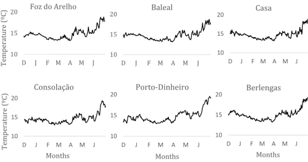
The environmental variables monitored in this study have shown seasonal patterns, as much as we could see during the sampling period. The sea surface temperature had relatively the same evolution during the sampling months in every sampling sites, showing a typical increase in temperatures from winter to spring with mean minimum temperatures around 13.35 ºC in February and mean maximum temperatures of 17.32 ºC in June (Figure 7).
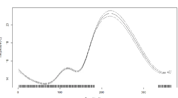
A Generalized Additive Model (GAM), Table 1, was performed to identify temperature seasonality and variability inter-locations using the day of the year and location as explanatory variables. Both variables demonstrated a significant relationship, explaining 84.9% of the variability observed (GAM, Table 1, Figure 8). Regarding to location, the baseline applied to perform it was Baleal. The temperature in Baleal was similar to every locations (p>0.05) except Consolação and Berlengas (p<0.001). Consolação on average was colder than the rest of sampling sites, while Berlengas was regularly warmer than the rest of the locations. The seasonal pattern (Figure 8) shows lower temperatures during the winter and a
10 15 20 D J F M A M J Te mpe ra ture ( ºC ) Foz do Arelho 10 15 20 D J F M A M J Baleal 10 15 20 D J F M A M J Casa 10 15 20 D J F M A M J Te mpe ra tu re ( ºC ) Months Consolação 10 15 20 D J F M A M J Months Porto-Dinheiro 10 15 20 D J F M A M J Months Berlengas
Figure 7 - Evolution of temperature during the sampling months in the different sampling locations.
30 typical increase in temperature during the spring-summer, although the lack of data between July and November.
Table 1 - Structure of the General Additive Model selected to describe Temperature. S.E.:
standard error; e.d.f.: estimated degrees of freedom.
Parametric coefficients Estimate Std. Error t Pr(>|t|)
Intercept (Baleal) 14.786 0.034 429.037 <2x10-16 *** Casa -0.014 0.048 -0.278 0.781 Consolação -0.189 0.048 -3.868 1.2x10⁻⁴ *** Berlengas 0.260 0.048 5.332 1.15x10⁻⁷ *** Foz do Arelho 0.034 0.048 0.705 0.481 Porto Dinheiro -0.01 0.048 -0.207 0.836 Approximate significance
of smooth terms edf F p-value
s(YearDay) 8.958 780.5 <2x10-16 ***
Figure 8 - Result of the Generalized Additive Models (GAM), showing the partial effect of Day of the Year on Temperature. Dotted lines indicate 95% confidence intervals, and tick marks along the X-axis below each curve represent effect values where observations occurred.
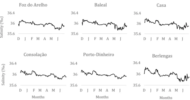
31 The evolution of salinity along the months was similar in the 6 locations (Figure 9). There was almost no variation, with mean minimum values of salinity around 35.83‰ in May and mean maximum values of approximately 36.14‰ in December.
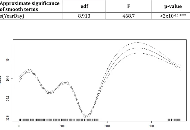
A GAM, Table 2, was performed to identify salinity seasonality and variability between locations using the day of the year and location as explanatory variables. Both variables demonstrated a significant relationship, explaining 77.9% of the variability observed. The baseline applied to perform it was Baleal, regarding to location. The salinity in Baleal, Berlengas and Foz do Arelho was similar (p>0.05) and Casa, Consolação and Porto Dinheiro had on average higher values of salinity than Baleal (p<0.01). The seasonal pattern (Figure 10) shows a typical decrease in salinity during winter-spring and predicts an increase during the summer, although we have no data between July and November.
35.6 36 36.4 D J F M A M J Salini ty (‰ ) Foz do Arelho 35.6 36 36.4 D J F M A M J Baleal 35.6 36 36.4 D J F M A M J Casa 35.6 36 36.4 D J F M A M J Salini ty (‰ ) Months Consolação 35.6 36 36.4 D J F M A M J Months Porto-Dinheiro 35.6 36 36.4 D J F M A M J Months Berlengas
Figure 9 - Evolution of salinity during the sampling months in the different sampling locations.
32
Table 2 – Structure of the General Additive Model selected to describe Salinity. S.E.:
standard error; e.d.f.: estimated degrees of freedom.
Parametric coefficients Estimate Std. Error t Pr(>|t|)
Intercept (Baleal) 35.963 0.003 12174.577 <2x10-16 *** Casa 0.017 0.004 4.012 6.37x10⁻⁵ *** Consolação 0.013 0.004 3.034 0.00246 ** Berlengas 0.007 0.004 1.686 0.09209 . Foz do Arelho -0.007 0.004 -1.742 0.08176 . Porto Dinheiro 0.022 0.004 5.327 1.18x10⁻⁷ *** Approximate significance
of smooth terms edf F p-value
s(YearDay) 8.913 468.7 <2x10-16 ***
The concentration of Chl-a (Figure 11) had some differences between the sampling sites. The peaks of concentration occurred simultaneously in every locations, in the end of March and in May, however with very different scales. In the Berlengas Natural Reserve, the major peak in the end of March only reached 4.56 mg/m³, and stayed below 1mg/m³ the rest of the months. In Baleal and Casa the peaks were higher, with 10.67 mg/m³ and 9.13 mg/m³ respectively in end of March, and 7.65 mg/m³ and 4.26 mg/m³ respectively in May. In Foz do Arelho and Porto-Dinheiro, the higher values were 17.42 mg/m³, and 14.57 mg/m³ correspondingly,
Figure 10 - Result of the Generalized Additive Models (GAM), showing the partial effect of
Day of the Year on Salinity. Dotted lines indicate 95% confidence intervals, and tick marks along the X-axis below each curve represent effect values where observations occurred.
33 in early spring and 14.47 mg/m³ and 15.21 mg/m³ in May. Consolação has the higher concentrations of Chl-a with a first peak in March of 13.06 mg/m³ and a major one in May with 42.37 mg/m³.
The concentration of Chl-a did not show such a relevant seasonal pattern. The GAM, only explains 10% of variability using the Day of the Year and Location as explanatory variables, but we can still detect the typical spring maximum, spring transition (Figure 12). Regarding to locations, Baleal was applied as the baseline (Table 3). The concentration of Chl-a in Baleal was similar to Casa and Porto Dinheiro (p>0.05). Consolação and Foz do Arelho have shown higher values of
Chl-a (p<0.5), Chl-and both locChl-ations in the BerlengChl-as IslChl-and (BuzinChl-as Chl-and Forte) showed
significantly lower values (p<0.001). 0 20 40 D J F M A M J Ch l a ( m g/m³ ) Foz do Arelho 0 20 40 D J F M A M J Baleal 0 20 40 D J F M A M J Casa 0 20 40 D J F M A M J Ch l a ( m g/m³ ) Months Consolação 0 20 40 D J F M A M J Months Porto-Dinheiro 0 20 40 D J F M A M J Months Berlengas
Figure 11 - Evolution of Chl-a concentration (mg/m³) during the sampling months in the
34
Table 3 - Structure of the General Additive Model selected to describe the Concentration of
Chl-a. S.E.: standard error; e.d.f.: estimated degrees of freedom.
Parametric coefficients Estimate Std. Error t Pr(>|t|)
Intercept (Baleal) 1.570 0.124 12.631 <2x10-16 *** Buzinas -0.722 0.176 -4.105 4.27x10⁻⁵ *** Casa -0.101 0.176 -0.575 0.566 Consolação 0.426 0.176 2.424 0.015 * Forte -0.759 0.176 -4.316 1.7x10⁻⁵ *** Foz do Arelho 0.607 0.176 3.451 5.74x10⁻⁴ *** Porto Dinheiro 0.144 0.176 0.815 0.415 Approximate significance
of smooth terms edf F p-value
s(YearDay) 3.541 17.71 1.52x10⁻¹³ ***
The upwelling index is represented in Figure 13A from September 2013 to June 2014. We could analyse that from September 2013 until the next spring, in May 2014, downwelling events were preponderant, although with some upwelling peaks (in November 2013, and January 2014). From May 2014 onwards, upwelling events turns more prevalent, matching upwelling seasonality in these latitudes (upwelling
Figure 12 - Result of the Generalized Additive Models (GAM), showing the partial effect of
Day of the Year on the Concentration of Chl-a. Dotted lines indicate 95% confidence intervals, and tick marks along the X-axis below each curve represent effect values where observations occurred.
35 predominant winds from spring to early-autumn, and downwelling predominant winds during the rest of the year).
The higher temperatures and low Chl-a concentrations registered in Berlengas Archipelago with respect to the rest of the sampling locations, might be indicating the presence of an upwelling front between the Island and mainland. In order to identify the existence of that front and its relationship with upwelling, we have analysed the index DifTemp (i.e. the difference of temperature between Berlengas and each different locations in mainland) (Figure 13B), and its relation to the upwelling index and its persistence (UI averaged 5 and 10 days).
-2 -1.5 -1 -0.5 0 0.5 1 1.5 2 2.5 3 Temp er at u re d iffe rence (ºC ) Months
Baleal Casa Consolação FozdoArelho PortoDinheiro
B -11000 -8000 -5000 -2000 1000 4000 7000 Me an UI (m 3/s/km) A
Figure 13 - At the top (A) is represented the upwelling index (m3/s/km) from September 2013 to June 2014, while in the bottom (B) is the temperature difference (temperature of Berlengas minus the temperature of each mainland location - ºC), along the sampling months.
36 A GAM (Table 4, Table 5, and Figure 14) was performed in order to analyse that interaction between the upwelling index (mean of the previous 5 and 10 days) and the temperature difference in each mainland location in relation to Berlengas. Regarding to location, the baseline applied to perform the model was Baleal. This model could explain 17.7% and 20.5% of the variability observed (for the 5 and 10 days averaged UI respectively). UI10d and Location are the combination that explains better the variability observed in DifTemp, but using both analyses we can compare the differences between more prevalent up-down events and those which are less prevalent.
We could observe significant interactions between upwelling and the different locations (p<0.01, in both cases with the mean UI of the previous 5 and 10 days; Tables 4 and 5). For the places located to North of Cape Carvoeiro, Foz do Arelho and Baleal, we observed a linear relation between the difference of temperature and UI when UI > 0 (Figure 14A, B). The higher the upwelling index, the higher the difference in sea water temperature between Berlengas and those locations, both using the averaged upwelling index for 5 days or 10 days, which means that in Berlenga’s locations the temperature becomes higher in relation to Foz do Arelho and Baleal. That might indicate that even during persistent upwelling events (10 days) the upwelling front cannot reach the Island, and the water remains warmer in the Island than in the coastline. During downwelling events (i.e. negative values of UI), in Baleal there is almost no variation in temperature difference, although in Foz do Arelho the DifTemp increases to positive values once again (Figure 14A, B).
At Casa, located in the Cape Carvoeiro, the temperature difference increases to positive values with the upwelling index until it reaches a plateau, when we use the previous 5 days UI average (Figure 14C). When the previous 10 days UI average is used, the relation become more linear (Figure 14C), indicating that more persistent upwelling or downwelling events have a stronger effect in temperature differences at this location. With downwelling events of 5 days the temperature difference tend to zero, becoming similar in Berlengas and Casa. But with events of 10 days persisting, the difference of temperatures becomes linearly negative, indicating colder waters in the Island than in mainland.
37 In the locations south of the Cape, Consolação and Porto Dinheiro, also can be observed an increase in temperature differences during upwelling events until those differences reach a plateau (Figure 14D, E). When we look to more persistent upwelling events (mean previous 10 days UI), differences in temperature between the Island and southern locations tend to disappear when the upwelling index is high (Figure 14D, E). This might indicate some kind of recirculation of upwelled water south of the cape, which might reach the Island simultaneously to mainland only when upwelling index is strong and persistent. Nevertheless, when looking at 10 day averaged UI, Porto-Dinheiro also showed a particular behaviour. When intermittent upwelling is prevalent (mean UI 10d around 0) differences in temperature tend to be negative, with colder water closer to the island in relation to Porto Dinheiro (Figure 14E), this might indicate that the upwelled water under relaxation events, can reach the island.
Table 4 - Result of the Generalized Additive Models (GAM), showing the partial effect of Day
of the Year on Upwelling Index (mean of 5 previous days - m3 s-1 km-1) in the temperature difference at each mainland location. Dotted lines indicate 95% confidence intervals, and tick marks along the X-axis below each curve represent effect values where observations occurred.
Parametric coefficients Estimate Std. Error t Pr(>|t|)
Intercept (Baleal) 0.209 0.027 7.690 3.66x10⁻¹⁴ *** Casa 0.053 0.039 1.374 0.169 Consolação 0.140 0.039 3.630 2.98x 10⁻⁴ *** Foz do Arelho -0.066 0.039 -1.720 0.086 Porto Dinheiro -0.063 0.039 -1.644 0.100 Approximate significance
of smooth terms edf F p-value
s(mean5d):Baleal 1.968 5.219 3.27x10⁻³ **
s(mean5d):Casa 3.037 3.915 4.55x10⁻³ **
s(mean5d):Consolação 5.217 8.415 3.26x10⁻⁹ ***
s(mean5d):FozdoArelho 2.981 5.294 5.2x10⁻⁴ ***
38
Table 5 - Result of the Generalized Additive Models (GAM), showing the partial effect of Day
of the Year on Upwelling Index (mean of 10 previous days - m3 s-1 km-1) in the temperature difference at each mainland location. Dotted lines indicate 95% confidence intervals, and tick marks along the X-axis below each curve represent effect values where observations occurred.
Parametric coefficients Estimate Std. Error t Pr(>|t|)
Intercept (Baleal) 0.209 0.027 7.795 1.73x10⁻¹⁴ *** Casa 0.056 0.038 1.473 0.141 Consolação 0.130 0.038 3.436 6.16x 10⁻⁴ *** Foz do Arelho -0.071 0.038 -1.885 0.059 Porto Dinheiro -0.089 0.038 -2.368 0.018 * Approximate significance of
smooth terms edf F p-value
s(mean10d):Baleal 1.373 1.653 2.2x10⁻³ **
s(mean10d):Casa 1.000 1.000 8.41x10⁻³ **
s(mean10d):Consolação 5.477 6.626 6.18x10⁻¹⁰ ***
s(mean10d):FozdoArelho 3.453 4.300 2.29x10⁻³ **
39 A B C D E
Figure 14 - Result of the Generalized Additive Models (GAM), showing the partial effect of
Upwelling Index averaged during the last 5 and 10 days (m3 s-1 km-1) in the temperature difference (ºC) at each mainland location (from top to bottom, in the same way as from North to South: A) Foz do Arelho, B) Baleal, C) Casa, D) Consolação, E) Porto-Dinheiro). Dotted lines indicate 95% confidence intervals, and tick marks along the X-axis below each curve represent effect values where observations occurred.
40
Settlement time series (monthly sampling)
Different temporal and spatial patterns of Mytilus galloprovincialis densities per sampled area were observed according to the range of sizes considered.
Recently arrived individuals, with less than 15 days and with mean size less than 0.6 mm (Figure 15), show a common and intense peak in the beginning of May, except for the locations in the reserve island (Forte and Buzinas), which had the highest density in the end of winter (February and March) with 18.67±22.85 and 26.0±43.31 individuals/square, respectively. These two locations also had a second and smallest peak in the beginning of May with 9.0±7.94 e 9.67 ±8.62 indiv/square, in Forte and Buzinas respectively.
The values of mussel settlement were considerably higher in Foz do Arelho with 419±92.72 indiv/square in May and 109.67±96.67 indiv/square in June, while in winter and early spring settlement was almost inexistent. In Porto-Dinheiro early settlers had a maximum of density in June with 96.67±73.53 indiv/square and before in May with 91.33±71.06 indiv/square, and during the winter some settlement was registered with 12.60±11.55 indiv/square in December and 13±5.57
0 10 20 30 40 50 60 70 80 90 100 D J F M A M J Nu mb er o f i ndi vi du als /sample d ar ea Baleal Buzinas Casa Consolação Forte Porto-Dinheiro 0 50 100 150 200 250 300 350 400 450 D J F M A M J Foz do Arelho < 0.6 mm
Figure 15 - Settlement time series, with the number of individuals with less than 0.600 mm
per sampled area (36cm²), between December 2013 and June 2014, in every sampling location. On the left are represented Buzinas, Forte, Baleal, Casa, Consolação and Porto-Dinheiro. On the right is only Foz do Arelho, with a totally different scale.
41 indiv/square in February. In Baleal the maximum of density was observed in May with 50.67±9.61 indiv/square, and with almost no record of early settlers in the rest of the sampling months, except in February with 6.33±6.11 indiv/square. Consolação had a maximum mean of settlement in May with 17.67±7.37 indiv/square, but also have shown similar values in March with 13.33±7.57 indiv/square. At the site located on the edge of the Peniche’s peninsula, Casa, was recorded a maximum density of early settlers in May, although very reduced, with only 5.67±6.03 indiv/square.
The maximum correlations between settlement time series were found between Consolação and Casa, at lag0 (r=0.99). Another locations also presented maximum correlations at lag0, as Baleal and Foz do Arelho (r=0.95), Baleal and Casa (r=0.77), Casa and Foz do Arelho (0.77), and Foz do Arelho and Porto-Dinheiro (r=0.88). Buzinas, located in the Berlengas Island, have shown maximum correlations at lag+2 with Baleal and Foz do Arelho (r=0.94 and r=0.88, respectively). There weren’t found any significant correlations between the rest of the locations.
In the scaled abundance of the individuals with less than 0.6 mm (Figure 16), similar results to the cross-correlations can be observed, although represented in an easier way. The peaks of abundance can be detected in different locations in winter and in spring, meaning that settlement is not synchronized among stations. During the winter the maximum abundances predominate in the southern locations and in the island (Consolação, Porto-Dinheiro, Buzinas and Forte). In the other hand, when spring begins can be observed a shift of the maximum abundances to the northern locations (Baleal, and mainly Foz do Arelho).
42 0.0 0.5 1.0 Sca led ab u n d an ce 12/2013
(<0.6 mm)
0.0 0.2 0.4 0.6 0.8 1.0 Sca led ab u n d an ce 02/2014 0.0 0.5 1.0 Sca led ab u n d an ce 03/2014 0.0 0.5 1.0 Sca led ab u n d an ce 04/2014 0.0 0.5 1.0 Sca led ab u n d an ce 05/2014 0.0 0.5 1.0 Sca led ab u nd anc e Locations 06/2014Figure 16 - Scaled abundance of the early settlers (<0.6 mm) in every locations, between
43 When analysing the time series of the second group mean density, a totally different pattern can be found (Figure 17). This group with the individuals comprehended between 0.6 mm and 2 mm, can be defined as plantigrades (Bayne 1976). Based on the growth rates calculated, these individuals are around 1-2 months old.Unlike early settlers, plantigrades have shown a clear high mean density in December, at least in 3 locations (Buzinas, Forte e Porto-Dinheiro), suggesting that in this 3 sites the settlement peak in Autumn is of great importance, while in the other locations (Foz do Arelho, Baleal, Casa and Consolação) it seems to have no relevance.
In all the sampling sites was registered a higher mean density of individuals between 0.600 mm and 2 mm than of early settlers, in almost every months. Once this range of sizes comprehend individuals between 1 and 2 months old, each monthly samplings integrates individuals that arrived in the last 2 months, while the group of early settlers (<0.6 mm) arrived no more than 15 days ago.
In Baleal, the maximum density appears earlier now in February with 71±74.22 indiv/square. In Casa, the maximum appears in December with 56.25±32.42 indiv/square, although the mean density in the rest of the months
0 50 100 150 200 250 300 350 400 D J F M A M J Nu mb er o f i ndi vi du als /sample d ar ea Baleal Buzinas Casa Consolação Forte Porto-Dinheiro 0 200 400 600 800 1000 1200 D J F M A M J Foz do Arelho 0.6 - 2 mm
Figure 17 - Settlement time series, with the number of individuals between 0.600 mm and
2 mm, per sampled area (36cm²), between December 2013 and June 2014, in every sampling location. On the left are represented Buzinas, Forte, Baleal, Casa, Consolação and Porto-Dinheiro. On the right is only Foz do Arelho, with a totally different scale.
44 doesn’t show much variation. In Consolação, appears a clear peak of mean density in March, with 161.33±15.63 indiv/square. Foz do Arelho has a larger peak with 1202.33±918.82 indiv/square, in June, one month later than the peak of early settlers. Porto-Dinheiro have shown a maximum density of plantigrades in December 330.80±167.91 indiv/square, decreasing until April, increasing again until the next peak in June with 250.67±81.88 indiv/square. In the Berlengas Natural Reserve, the peak in December is also evident, with 379.33±155.09 in Buzinas and 324.60±168.70 in Forte. In Buzinas a second peak happens in March (259.33±144.97 indiv/square), and in Forte after decreasing until April, a second smaller peak appears with 134.33±97.30 indiv/square in May.
Analysing the cross-correlations between the settlement time series of plantigrades in the Berlengas Natural Reserve and neighbour areas, a maximum correlation at lag0 can be found between the Island locations Forte and Buzinas (r=0.85). Maximum and significant correlations at lag0 were also found between Casa and Forte (r=0.85), Casa and Buzinas (r=0.75), and also between Porto-Dinheiro and Buzinas (r=0.75). Moreover, at lag+1 a significant correlation between Baleal and Porto-Dinheiro was registered (r=0.81).
In Figure 18, the scaled abundance of the individuals with length between 0.6 and 2 mm presents a similar pattern to the early settler’s. With maximum abundances in the southern locations and in the island during winter, and during spring the maximums are presented in the northern locations.