Modeling stock markets' volatility using GARCH models with normal, Student's t and stable Paretian distributions

Repositório ISCTE-IUL

Deposited in Repositório ISCTE-IUL:

Deposited version:

Peer-review status of attached file:

Citation for published item:

Curto, J., Pinto, J. C. & Tavares, G. N. (2009). Modeling stock markets' volatility using GARCH models with normal, Student's t and stable Paretian distributions. Statistical Papers. 50 (2), 311-321

Further information on publisher's website:

Publisher's copyright statement:

This is the peer reviewed version of the following article: Curto, J., Pinto, J. C. & Tavares, G. N. (2009). Modeling stock markets' volatility using GARCH models with normal, Student's t and stable Paretian distributions. Statistical Papers. 50 (2), 311-321, which has been published in final form at https://dx.doi.org/10.1007/s00362-007-0080-5. This article may be used for non-commercial purposes in accordance with the Publisher's Terms and Conditions for self-archiving.

Use policy

Creative Commons CC BY 4.0

The full-text may be used and/or reproduced, and given to third parties in any format or medium, without prior permission or charge, for personal research or study, educational, or not-for-profit purposes provided that:

• a full bibliographic reference is made to the original source • a link is made to the metadata record in the Repository • the full-text is not changed in any way

The full-text must not be sold in any format or medium without the formal permission of the copyright holders.

Serviços de Informação e Documentação, Instituto Universitário de Lisboa (ISCTE-IUL) Av. das Forças Armadas, Edifício II, 1649-026 Lisboa Portugal

Phone: +(351) 217 903 024 | e-mail: administrador.repositorio@iscte-iul.pt https://repositorio.iscte-iul.pt

This is an Author's Accepted Manuscript of an article published as: CURTO J.D., PINTO J.C. and TAVARES, G.N. (2009) Modeling stock markets’ volatility using GARCH models with Normal, Student’s t and stable Paretian distributions. Statistical Papers, 50(2), 311-321 available online at:

(will be inserted by the editor)

Modeling stock markets’ volatility using

GARCH models with Normal, Student’s t

and stable Paretian distributions

Jos´e Dias Curto1_{, Jos´e Castro Pinto}1_{, Gon¸calo Nuno Tavares}2

1 _{ISCTE Business School, Department of Quantitative Methods, Complexo}

IN-DEG/ISCTE, Av. Prof. An´ıbal Bettencourt, 1600-189 Lisboa, Portugal. Phone:

351 21 7826100. Fax: 351 21 7958605. E-mail: dias.curto@iscte.pt.

2 _{Instituto de Engenharia de Sistemas e Computadores - Investiga¸c˜ao e}

Desen-volvimento (INESC-ID), Lisbon and Department of Electrical and Computer

Engineering, Instituto Superior T´ecnico (IST), Lisbon.

Received: date / Revised version: date

Abstract As GARCH models and stable Paretian distributions have been revisited in the recent past with the papers of Hansen and Lunde (2005) and Bidarkota and McCulloch (2004), respectively, in this paper we dis-cuss alternative conditional distributional models for the daily returns of the US, German and Portuguese main stock market indexes, considering ARMA-GARCH models driven by Normal, Student’s t and stable Paretian distributed innovations. We find that a GARCH model with stable Paretian

innovations fits returns clearly better than the more popular Normal distri-bution and slightly better than the Student’s t distridistri-bution. However, the Student’s t outperforms the Normal and stable Paretian distributions when the out-of-sample density forecasts are considered.

Key words Non-Gaussian distributions, Conditional heteroskedasticity.

1 Introduction

Since the birth of the modern empirical finance two main approaches have been considered to model the empirical distribution of financial assets re-turns. The first one, that we name the unconditional approach, admits that stock prices follow a random walk and several models have been proposed to describe the unconditional distribution of financial returns.

However, as the empirical findings suggest the presence of volatility clus-ters, one might represent this kind of returns behavior using a model where the conditional variance is serially correlated and since the seminal paper of Engle (1982) was published, the second one, that we name the conditional approach, became common in empirical finance.

The unconditional approach is based on the assumption that location and scale parameters are constant, implying that returns are independent and identically distributed (i.i.d.) random variables. The Gaussian distri-bution was the first to be considered and the normality became one of the most important assumptions in the classical financial models, namely the Portfolio Theory, the Capital Asset Pricing Model (CAPM) and the

Black-Scholes’ formula. The Gaussian hypothesis was not seriously ques-tioned until the seminal papers of Mandelbrot (1963) and Fama (1965) were published. Since then, numerous studies have found that the empirical distribution of returns on financial assets exhibit fatter tails and are more peaked around the center than would be predicted by a Gaussian distri-bution. Thus, alternative distributions possessing such characteristics have been proposed as models for the unconditional distribution of returns. Man-delbrot (1963) attempted to capture the excess of kurtosis by modeling the returns distribution as a member of stable-L´evy or stable Paretian distrib-utions, where the Gaussian distribution is a special case. Other researchers have proposed alternative distributions like the Student’s t (Blattberg and Gonedes 1974), the GED: Generalized Error Distribution (Box and Tiao 1962), the Laplace and double Weibull (Mittnik and Rachev 1993).

On the other hand, the conditional approach admits temporal dependen-cies in the returns series allowing the financial modeling based frequently on past information. Traditionally, serial dependence in time series has been modeled with ARMA (Autoregressive Moving Average) structures, as this class of models provides a good specification for the conditional mean. How-ever, given the homoskedastic nature of the conditional distribution implicit in these models, they are unable to capture the volatility clustering that is common in financial asset returns.

As heteroskedasticity is a common characteristic of returns, and given the importance of predicting volatility in many asset-pricing and portfolio

management problems, different solutions for conditional modeling of re-turns have been proposed in the literature. As the high-frequency financial data exhibits volatility clustering, i. e., large (small) price changes tend to be followed by large (small) changes of either sign (Mandelbrot 1963), the most popular one is the class of Autoregressive Conditional Heteroskedas-ticity (ARCH) models originally introduced by Engle (1982) and latter Generalized (GARCH) by Bollerslev (1986), possibly in combination with an ARMA specification for the mean equation, referred to as an ARMA-GARCH model.

In its standard form GARCH models assume that the conditional distri-bution of assets returns is Gaussian. However, for many financial time series, this model specification does not adequately account for leptokurtosis. Thus, several non-Normal alternative distributions have been proposed. Bollerslev (1987) suggests using the Student’s t distribution. Nelson (1991) proposed the GED, the Laplace distribution has been employed in Granger and Ding (1995) and Hsieh (1989) used both Student’s t and GED as distributional alternative models for innovations. The stable Paretian distributions have been also investigated by Liu and Brorsen (1995), Panorska et al. (1995) and Mittnik et al. (1998, 2003).

In this paper we examine the conditional distribution of daily returns in the US, the German and the Portuguese equity markets, comparing the sta-ble Paretian distribution to the Gaussian and the Student’s t distributions for innovations. The Portuguese market is smaller, more recent and less

liq-uid. The German market is representative of intermediary markets, with a longer history but its role on the economy is lower than typical Anglosaxon capital markets. Finally, these markets were compared with the American market, the most liquid and one of the oldest in the World.

The paper is organized as follows. Next section provides a brief descrip-tion of the GARCH model with Normal, Student’s t and stable Paretian innovations. Section 3 describes the returns and presents some prelimi-nary findings. Section 4 discusses the estimation results and compares the goodness-of-fit of the three conditional distributions. Section 5 presents the out-of-sample evaluation results and the final section summarizes our con-cluding remarks.

2 The models

As it was referred before, ARMA models can be used to explain the condi-tional mean of the process based on past realizations:

rt= c + p X i=1 φirt−i+ q X i=1 θiut−i+ ut, (1)

where utis a white noise process and rtis return at time t.

GARCH models are commonly used to capture the volatility clusters of returns and express the conditional variance as a linear function of past information, allowing the conditional heteroskedasticity of returns. In its standard version, GARCH models are assumed to be driven by normally

distributed innovations (Bollerslev, 1986): σ2t = α0+ r X i=1 αiu2t−i+ s X i=1 βiσ2t−i and ut|Φt−1∼ N ¡ 0; σ2t ¢ , (2) where σ2

t, the scale parameter, represents the conditional variance of the process at time t, ut= εtσtand Φt−1= { ut−1, ut−2, ...}.

In addition to the normal GARCH model, we also consider two other specifications assuming Student’s t [εt ∼ t (v), where t (v) refers to the zero-mean t distribution with v degrees of freedom and scale parameter equal to one] and stable Paretian innovations. The parameterization and the properties of the stable Paretian GARCH model are discussed next. The more detailed description of this model is due to its less frequent use to modeling the conditional distribution of financial assets returns.

A process rtis called a stable Paretian GARCH, Sα,βGARCH (r, s), if it is described by (1) (Liu and Brorsen 1995, Panorska et al. 1995 and Mittnik et al. 1998) and, σt= α0+ r X i=1 αi| ut−i| + s X i=1 βiσt−i, (3)

where σt is the scale parameter of the process at time t, ut = σtεt, and εt are i.i.d. realizations of a stable Paretian distributed random variable with α > 1: εt iid∼ Sα,β. Sα,β represents the standard asymmetric sta-ble Paretian distribution with stasta-ble index α ∈ (0; 2], skewness parameter β ∈ [−1; 1], zero location parameter and unit scale parameter. From the several notational alternatives of the stable Paretian distribution we select the parameterization suggested by Samorodnitsky and Taqqu (1994) and

Rachev and Mittnik (2000), whereby E¡eitX¢=       

exp©i t − | t|α£_{1 − iβ tan}πα

2 sign (t) ¤ª , if α 6= 1 exp©i t − | t|£1 + iβ2 πsign (t) ln | t| ¤ª , if α = 1 (4)

is the characteristic function.

The distribution is symmetric about the zero location parameter if β = 0 and the characteristic exponent α determines the total probability in the ex-treme tails of the distribution. When α = 2, the underlying stable Paretian distribution is the Normal distribution: N (0; 2), with finite moments of all orders. As α decreases from 2 to 0, the tail areas of the stable distribution become increasingly fatter than the Normal. For α < 2, the sth _absolute moment exists only for s < α and, except for the Normal case, the stable Paretian distribution has infinite variance. Thus, the analog of the variance in this kind of distributions is the scale parameter σt. In this paper we assume that α > 1, the necessary condition for the existence of the mean.

The Sα,βGARCH (r, s) process defined by (1) and (3) with 1 < α < 2 has a unique strictly stationary solution if αi > 0, i = 0, ..., r, βi > 0, i = 1, ..., s and the measure of volatility persistence, VS = λα,β

r P i=1 αi+ s P j=1 βj, satisfies VS ≤ 1 (Rachev and Mittnik 2000), where

λα,β = E |εt| = 2 πΓ µ 1 − 1 α ¶ ¡ 1 + τα,β2 ¢1 2α_cos µ 1 αarctan τα,β ¶ , (5) with τα,β= β tanαπ 2 .

If Vs is strictly less than one, this implies a conditional volatility equa-tion where the impact of a shock dies out over time. If VS = 1, analo-gous to the ordinary normal GARCH model, we say that rt is an

inte-grated Sα,βGARCH (r, s) process, denoted by Sα,βIGARCH (r, s), which implies non-decaying effects of shocks on the conditional volatility (Engle and Bollerslev 1986). In practice, the estimated volatility persistence, ˆVS, tends to be quite close to one for highly volatile series and the integrated model might offer a reasonable data description.

3 Statistical properties of returns

The data consists of daily closing prices of DJIA, DAX and PSI20 indexes, which are main market indexes for the US, German and Portuguese equity markets. These series cover the period from December 31, 1992 to December 31, 2006 yielding 3527, 3565 and 3518 observations, respectively. We analyze the continuously compounded percentage rates of return (not adjusted for dividends) that are calculated by taking the first differences of the logarithm of series (Pt is the closing value for each stock index at time t):

rt= 100 × [ln (Pt) − ln (Pt−1)] . (6)

Table 1 summarizes the basic statistical properties of the data. The means returns are all positive but close to zero. The returns appear to be somewhat asymmetric as reflected by negative skewness estimates. All three series returns have heavy tails and show strong departure from normality (skewness and kurtosis coefficients are all statistically different from those of the standard Normal distribution which are 0 and 3, respectively). The Jarque-Bera test also clearly rejects the null hypothesis of normality.

Table 1 Summary statistics of returns

Statistics DJIA DAX PSI20 No. of observations 3527 3565 3518 Mean 0.037667 0.040936 0.037439 Median 0.049530 0.103311 0.037463 Maximum 6.154722 7.552676 6.941259 Minimum -7.454935 -8.882302 -9.589772 Standard deviation 1.001393 1.444509 0.989100 Skewness -0.227090 -0.259241 -0.630273 Kurtosis 7.748924 6.474062 11.13506 JBa _{3344.56* 1832.70* 9933.68*} LB Q(10)b _{15.021 12.77 124.22*} LB Q2₍₁₀₎c _{916.56* 2375.90* 849.61*} ARCH(1) LMd _{110.14* 185.06* 202.42*}

* Denotes significant at the 1% level,

a _{JB is the Jarque Bera test for normality,} b _{LB Q(10) is the Ljung-Box test for returns,}

c _{LB Q}2_{(10) is the Ljung-Box test for squared returns,}

d _{LM is the Engle’s Lagrange Multiplier test for heteroskedasticity.}

According to the Ljung-Box statistic for returns, there is no relevant autocorrelation for the DAX and the DJIA indexes. For PSI20, however, returns have statistically significant first order autocorrelation, which can be removed by fitting an autoregressive AR(1) model to this series. The successive returns correlation must be due to the market thinness and non-synchronous trading that is common in many small capital markets.

Even though the series of returns seems to be serially uncorrelated over time, the Ljung-Box statistic for up to tenth order serial correlation of squared returns is highly significant at any level for the three stock

in-dexes, suggesting the presence of strong nonlinear dependence in the data. As non-linear dependence and heavy-tailed unconditional distributions are characteristic of conditionally heteroskedastic data, the Lagrange Multiplier test (Engle, 1982) can be used to formally test the presence of conditional heteroskedasticity and the evidence of ARCH effects. The LM test for a first-order linear ARCH effect (in the last row of table 1) suggests that all stock indexes’ returns exhibit ARCH effects, implying that nonlineari-ties must enter through the variance of the processes (Hsieh, 1989). Such behavior can be captured by incorporating ARCH or GARCH structures in the model, allowing conditional heteroskedasticity by conditioning the volatility of the process on past information. In the next section we use ARMA-GARCH models to describe the conditional distribution of returns.

4 Modeling the empirical distribution of returns

In order to evaluate in-sample and out-of-sample results, the data sample is divided in two parts. One part is used for the in-sample models’ estimation; the other part is for the models’ performance out-of-sample evaluation. We consider the nine first years of observations to estimate the models (from De-cember 1992 to DeDe-cember 2001, yielding 2268, 2290 and 2226 observations for DJIA, DAX and PSI20, respectively). For the out-of-sample analysis we use the remaining observations comprising the years from 2002 to 2006 (the number of observations is 1259, 1275 and 1292, respectively). In this section we discuss in-sample estimation results.

The ARMA p and q orders (p = q = 0 for DJIA, DAX and p = 1, q = 0 for PSI20) were determined by the inspection of the sample autocorrelation function (SACF) and the sample partial autocorrelation function (PSACF) of the returns series (not shown in the paper). As is common in financial modeling (see Hansen and Lunde 2005 and Bollerslev et al. 1992) it was found that a GARCH(1,1) specification was adequate to capture the corre-lation in the squared returns.

The parameters were jointly estimated using conditional ML1_{, and it was} assumed that the scaled innovations, ut, are either Normal, Student’s t and stable Paretian and σtsatisfies GARCH recursions (2) and (3), respectively. As there is no analytical expression for the stable Paretian density, the ML estimation is approximate once the density function needs to be approxi-mate. We follow the algorithm of Mittnik et al. (1999) which approximates the stable Paretian density through fast Fourier transform (FFT) of the characteristic function.

To compare unconditional and conditional in-sample fitted models, we employ three likelihood based goodness-of-fit criteria proposed by Mittnik and Paolella (2003). The first is the maximum log-likelihood value obtained from ML estimation (L). This value allows us to judge which model is more likely to have generated the data. The second is the bias-corrected Akaike (Hurvich and Tsai 1989) information criteria (AICC) and the third is the

Schwarz Bayesian criteria (SBC): AICC = −2 log L ³ ˆ θ ´ +2n (k + 1) n − k − 2, SBC = −2 log L ³ ˆ θ ´ +k ln(n) n , (7) where log L ³ ˆ θ ´

is the maximum log-likelihood value, n is the number of observations and k is the number of parameters. The distribution with a lower value for these information criteria is judged to be preferable. These criteria are also recommended by Sin and White (1996).

To evaluate the goodness-of-fit improvement when the conditional struc-ture is adopted, first we compute the goodness-of-fit measures for the un-conditional distributions (not shown in the paper). The Student’s t model provides much closer approximation to the empirical unconditional density of PSI20 and DAX returns than Normal and stable Paretian. On the other hand, the stable Paretian model is favored quite strongly for DJIA returns with the largest maximized log-likelihood value and the smallest value for both AICC and SBC information criteria.

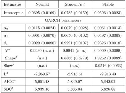
The estimation results of the returns’ conditional distribution are re-ported in tables 2, 3 and 4.

These results suggest some important conclusions regarding the uncon-ditional and conuncon-ditional distributions of returns. All the estimated coeffi-cients are significant at the 5% level. When compared to their unconditional counterparts, the improvement in fit obtained by adopting the conditional models is substantial for each distribution and for all the three stock mar-ket indexes. For example, in the stable Paretian case, the maximum log-likelihood value increases from −3, 086.83 to −2, 913.43 in the case of DJIA,

Table 2 Maximum likelihood estimates and goodness-of-fit statistics of GARCH(1,1) for DJIA (standard errors are in parentheses)

Estimates Normal Student’s t Stable Intercept c 0.0695 (0.0169) 0.0785 (0.0159) 0.0596 (0.0023) GARCH parameters α0 0.0115 (0.0024) 0.0079 (0.0028) 0.0061 (0.0013) α1 0.0901 (0.0070) 0.0650 (0.0102) 0.0497 (0.0005) β1 0.9029 (0.0080) 0.9291 (0.0107) 0.9325 (0.0018) Va _{0.9930 (n. a.) 0.9941 (n. a.) 0.9909 (0.0099)} Shapeb _{(n.a.) 6.8566 (0.8779) 1.9252 (0.0089)}

Skewc _{(n.a.) (n.a.) -0.9516 (0.0063)}

Ld _{-2,969.57 -2,915.51 -2,913.43}

AICCe _{5,951.18 5,849.07 5,842.92}

SBCf _{5,939.16 5,835.04 5,826.88} a _{V is the measure of volatility persistence: V = λα}

1+ β1 for the

Normal and Student’s t distributions and V = λα,βα1+ β1 for the

stable distribution, with λα,β given in eq. (5),

b _{“Shape” denotes the degrees of freedom parameter v for the}

Stu-dent’s t distribution and stable index α for the stable Paretian distri-bution,

c _{“Skew” refers to the stable Paretian skewness parameter β,} d _{L refers to the maximum log-likelihood value,}

e _{AICC is the bias-corrected Akaike Information Criterion,} f _{SBC is the Schwarz Bayesian Criterion.}

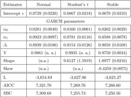
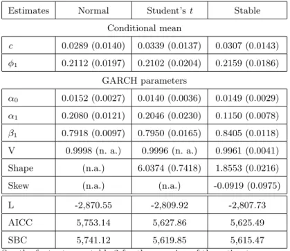
from −3, 836, 70 to −3, 625.27 in the case of DAX and from −3, 128.86 to −2, 807.73 in the case of PSI20.

The stable Paretian distribution, by contrast with the unconditional case for DAX and PSI20, achieves the largest likelihood value modeling the conditional distribution of all the stock market indexes’ returns, despite the small difference for the Student’s t. Consequently, the lower value of both information criteria and the maximum log-likelihood value indicate that the

Table 3 Maximum likelihood estimates and goodness-of-fit statistics of GARCH(1,1) for DAX (standard errors are in parentheses)

Estimates Normal Student’s t Stable Intercept c 0.0729 (0.0226) 0.0867 (0.0218) 0.0679 (0.0210) GARCH parameters α0 0.0281 (0.0049) 0.0160 (0.0061) 0.0202 (0.0029) α1 0.0923 (0.0097) 0.0781 (0.0116) 0.0588 (0.0078) β1 0.8939 (0.0106) 0.9154 (0.0126) 0.9058 (0.0108) V 0.9861 (n. a.) 0.9935 (n. a.) 0.9759 (0.0034) Shape (n.a.) 9.6127 (1.5919) 1.8977 (0.0216) Skew (n.a.) (n.a.) -0.4259 (0.0975) L -3,654.83 -3,627.86 -3,625.27 AICC 7,321.70 7,269.76 7,266.60 SBC 7,309.68 7,255.73 7,250.56 See the footnotes on table 2 for the meaning of the estimates.

GARCH(1,1) model with conditional stable Paretian distribution provides a better fit to describe the volatility of returns in the US, German and Portuguese equity markets.

The persistence-of-volatility estimates are very near one showing that conditional models for returns are very close to being integrated. Thus, we also estimated the distributional models with the IGARCH conditions imposed. Not surprisingly, as the persistence measure is close to unity, the IGARCH-restricted parameter estimates and the goodness-of-fit statistics differ very little when compared to non restricted models. This is the reason why the estimation results are not shown in the paper.

Table 4 Maximum likelihood estimates and goodness-of-fit statistics of AR(1)-GARCH(1,1) for PSI20 (standard errors are in parentheses)

Estimates Normal Student’s t Stable Conditional mean c 0.0289 (0.0140) 0.0339 (0.0137) 0.0307 (0.0143) φ1 0.2112 (0.0197) 0.2102 (0.0204) 0.2159 (0.0186) GARCH parameters α0 0.0152 (0.0027) 0.0140 (0.0036) 0.0149 (0.0029) α1 0.2080 (0.0121) 0.2046 (0.0230) 0.1150 (0.0078) β1 0.7918 (0.0097) 0.7950 (0.0165) 0.8405 (0.0118) V 0.9998 (n. a.) 0.9996 (n. a.) 0.9961 (0.0041) Shape (n.a.) 6.0374 (0.7418) 1.8553 (0.0216) Skew (n.a.) (n.a.) -0.0919 (0.0975) L -2,870.55 -2,809.92 -2,807.73 AICC 5,753.14 5,627.86 5,625.49 SBC 5,741.12 5,619.85 5,615.47 See the footnotes on table 2 for the meaning of the estimates.

5 Out-of-sample density forecasts

As we are testing non-Gaussian distributions for the underlying process of returns, we support the out-of-sample analysis in density forecasts (Poon and Granger, 2003). Thus, rather predicting first and second moments as is common in the GARCH literature, we focus on density predictions and the overall density forecasting performance of competing models can be compared by evaluating their conditional densities at the future observed values (Mittnik and Paolella, 2003):

ˆ ft+1|t(rt+1) = f  rt+1− µ ³ ˆ θt ´ σt+1 ³ ˆ θt ´ |rt, rt−1, . . .   , (8)

where ˆft+1|t(·) is the one-step-ahead density forecast, ˆθt refers to the es-timated parameters based on the sample information up to and including period t and σt+1 results from (2) and (3) by using ˆθt. We re-estimate (via ML estimation) the model parameters at each step, as is common in actual applications. Thus, 1258, 1274 and 1291 observations are used for DJIA, DAX and PSI20 out-of-sample density forecasts evaluation, respectively. A model will fare well in the comparison among competing models if realiza-tion rt+1is near the mode of ˆft+1|t(rt+1) and if the mode of the conditional density is more peaked (Mittnik and Paolella, 2003).

Table 5 presents the means, standard deviations and medians of the es-timated density values ˆft+1|t(rt+1). For all the three stock market indexes (except for DAX when the median is considered) the best performance is achieved by the Student’s t distribution when both central tendency mea-sures are used. Notice that this is contrary to the model selection based on the goodness-of-fit measures where the stable Paretian distribution had better in-sample performance to describe returns data.

6 Conclusions

In this paper we have discussed alternative unconditional and conditional distributional models for the daily returns of DJIA, DAX and PSI20 stock market indexes considering AR-GARCH models driven by Normal, Stu-dent’s t and stable Paretian distributed innovations.

Table 5 Comparison of overall predictive performance Distribution DJIA DAX PSI20 Mean Normal 0.3597 0.2562 0.4462 Student’s t 0.3733 0.2651 0.4776 Stable 0.2962 0.2339 0.3499 St. deviation Normal 0.1839 0.1471 0.2239 Student’s t 0.2101 0.1651 0.2726 Stable 0.1193 0.1110 0.1156 Median Normal 0.3571 0.2477 0.4419 Student’s t 0.3603 0.2509 0.4593 Stable 0.3228 0.2566 0.3747 The entries represent average predictive likelihood values.

The behavior of returns has the common characteristics of high-frequency financial time series. First, they exhibit a considerable level of excess kur-tosis. Second, nevertheless the small autocorrelation of returns, the serial dependence in the square returns is clearly not rejected pointing towards the existence of volatility clusters. Finally, the volatility of returns tends to be highly persistent.

When compared to their unconditional counterparts, the improvement in fit obtained by the conditional models is substantial for each distribution and for all the three stock market indexes.

By contrast with the unconditional case, where the Student’s t achieves the best fit for DAX and PSI20 returns, the stable Paretian distribution achieves the largest likelihood value modeling all the three conditional dis-tributions of returns, despite the small difference for the Student’s t. How-ever, in the out-of-sample analysis the best performance is also achieved by

the Student’s t distribution for all the three stock market indexes.

Acknowledgements

The authors would like to thank the editor and the referee whose thoughtful comments led to substantial improvements in the paper.

References

1. Akaike H (1978) Time series analysis and control through parametric models.

Applied Time Series Analysis. In: D. F. FINDLEY (Ed.), Academic Press,

New York

2. Bidarkota PV, McCulloch JH (2004) Testing for persistence in stock returns

with GARCH-stable shocks. Quantitative Finance 4, 256-265

3. Blattberg RC, Gonedes NJ (1974) A comparison of the Stable and Student

distributions as statistical methods for stock prices. Journal of Business 47,

244-280

4. Bollerslev T (1986) Generalized autoregressive conditional heteroskedasticity. Journal of Econometrics 31, 307-327

5. Bollerslev T (1987) A conditional heteroskedastic time series model for

spec-ulative prices and rates of return. Review of Economics and Statistics 69,

542-547

6. Bollerslev T, Chou RY, Kroner KF (1992) Arch modeling in finance. Journal

of Econometrics 52, 5-59

7. Box GEP, Tiao GC (1962) A further look at robustness via Bayes theorem.

8. Engle RF (1982) Autoregressive conditional heteroskedasticity with estimates of the variance of United Kingdom inflation. Econometrica 50 (4), 987-1006

9. Engle RF, Bollerslev T (1986) Modelling the persistence of conditional vari-ances. Econometric Reviews 5, 1-50

10. Fama EF (1965) The behavior of stock prices. Journal of Business 38, 34-105

11. Granger C, Ding Z (1995) Some properties of absolute return, an alternative measure of risk. Annales d’Economie et de Statistique 40, 67-91

12. Hansen PR, Lunde A (2005) A forecast comparison of volatility models: does anything beat a GARCH(1,1)? Journal of Applied Econometrics 20, 873-889

13. Hsieh, DA (1989) The statistical properties of daily foreign exchange rates: 1974-1983. Journal of International Economics 24, 129-145

14. Hurvich CM, Tsai CL 1989 Regression and time series model selection in small samples. Biometrika 76, 297-307

15. Jarque CM, Bera AK (1987) A test for normality of observations and

regres-sion residuals. International Statistical Review 55 (2), 163-172

16. Ljung GM, Box GEP (1978) On measure of lack of fit in time series models.

Biometrika 65, 297-303

17. Liu SM, Brorsen BW (1995) Maximum likelihood estimation of a

GARCH-stable model. Journal of Applied Econometrics 10, 273-285

18. Mandelbrot B (1963) The variation of certain speculative prices. Journal of

Business 36, 394-419

19. Mittnik S, Rachev S T (1993) Modeling asset returns with alternative stable

models. Econometric Reviews 12, 261-330

20. Mittnik S, Paolella MS, Rachev ST (1998) Unconditional and conditional

distributional models for the Nikkei Index. Asia-Pacific Financial Markets 5,

21. Mittnik S, Rachev ST, Doganoglu T, Chenyao D (1999) Maximum likelihood estimation of stable Paretian models. Mathematical and Computer Modeling

29, 275-293

22. Mittnik S, Paolella MS. (2003) Prediction of financial downside risk with

heavy-tailed conditional distributions. In: Handbook of Heavy Tailed

Distri-butions in Finance, Volume 1, Chapter 9, Elsevier North-Holland.

23. Nelson DB (1991) Conditional heteroskedasticity in asset returns: a new

ap-proach, Econometrica 59(2), 347-370

24. Panorska A, Mittnik S, Rachev ST (1995) Stable ARCH models for financial time series. Applied Mathematical Letters 8, 33-37

25. Poon S, Granger C (2003) Forecasting volatility in financial markets: a review.

Journal of Economic Literature 41, 478-539

26. Rachev S, Mittnik S (2000) Stable Paretian models in finance. John Wiley &

Sons, New York

27. Samorodnitsky G, Taqqu MS (1994) Stable non-Gaussian random processes.

Stochastic models with infinite variance. Chapman and Hall, London

28. Schwarz G (1978) Estimating the dimension of a model. Annals of Statistics 6, 461-64

29. Sin CY, White H (1996) Information criteria for selecting possibly misspecified