Adaptability and phenotypic stability of sugarcane clones
Jiuli Ani Vilas Boas Regis(1), João Antonio da Costa Andrade(1),
Adriano dos Santos(2), Aparecido Moraes(3), Rafael William Romo Trindade(1),
Hermano José Ribeiro Henriques(1), Bruno Henrique Polis(4) and Luiz Carlos Oliveira(4)
(1)Universidade Estadual Paulista Júlio de Mesquita Filho, Avenida Brasil, Centro, no 56, CEP 15385-000 Ilha Solteira, SP, Brazil. E-mail:
jiuli_regis@hotmail.com, jandrade@bio.feis.unesp.br, rafaelromo@live.com, hermano.henriques.hh@gmail.com (2)Universidade Estadual
do Norte Fluminense Darcy Ribeiro, Avenida Alberto Lamego, no 2.000, Parque Califórnia, CEP 28013-602 Campo dos Goytacazes, RJ,
Brazil. E-mail: adriano.agro84@yahoo.com.br (3)Universidade Federal de Lavras, Campus Universitário, Caixa Postal 3.037, CEP 37200-000
Lavras, MG, Brazil. E-mail: ap.de.moraes@bol.com.br (4)Centro de Tecnologia Canavieira, Santo Antônio, Caixa Postal 162, CEP 13400-970
Piracicaba, SP, Brazil. E-mail: bruno.polis@ctc.com.br, luiz.oliveira@ctc.com.br
Abstract – The objective of this work was to select superior sugarcane (Saccharum officinarum) clones with good stability and adaptability, considering the genotype x environment interaction in two productive cycles. Twenty-five early clones plus five control clones were evaluated during two cuts (ratoon cane and plant cane) in 24 environments. A randomized complete block design was used, with three replicates. Tons of stems per hectare and tons of pol per hectare were evaluated. To verify adaptability and stability, the bisegmented regression and the multivariate (AMMI and GGE biplot) methods were used. According to the three methods, which are complementary regarding the desired information, the most promising clones in terms of stability and general adaptability are G5, G12, and G13; the last two are closest to the ideal genotype. The G13 clone is highly productive in favorable and unfavorable environments, presenting the highest averages for ton of stems and pol per hectare. The G3, G4, G10, G15, G17, G18, G22, G23, G25, G26, and G30 clones are not recommended for the 24 evaluated environments.
Index terms: Saccharum officinarum, AMMI, genotype x environment interaction, GGE biplot.
Adaptabilidade e estabilidade fenotípicas de clones de cana-de-açúcar
Resumo – O objetivo deste trabalho foi selecionar clones de cana-de-açúcar (Saccharum officinarum) superiores, com boa estabilidade e adaptabilidade, ao se considerar a interação genótipo x ambiente em dois ciclos produtivos. Vinte e cinco clones precoces mais cinco clones testemunhas foram avaliados durante dois cortes (cana-soca e cana-planta), em 24 ambientes. Utilizou-se o delineamento experimental de blocos ao acaso, com três repetições. Foram avaliadas toneladas de colmos por hectare e toneladas de pol por hectare. Para a verificação da adaptabilidade e da estabilidade, foram utilizados os métodos de regressão bissegmentada e multivariados (AMMI e GGE biplot). De acordo com os três métodos, que são complementares nas informações desejadas, os clones mais promissores em termos de estabilidade e adaptabilidade geral são G5, G12 e G13; estes dois últimos são os mais próximos do genótipo ideal. O clone G13 é altamente produtivo nos ambientes favoráveis e desfavoráveis, tendo apresentado as maiores médias para tonelada de colmos e de pol por hectare. Os clones G3, G4, G10, G15, G17, G18, G22, G23, G25, G26 e G30 não são recomendados para os 24 ambientes avaliados.
Termos para indexação: Saccharum officinarum, AMMI, interação genótipo x ambiente, GGE biplot.
Introduction
Brazil has been the world’s largest producer of sugarcane (Saccharum officinarum L.) for more than 30 years, followed by India and China (OECD-FAO..., 2015). The agribusiness of this crop contributes effectively to the development of the country and represents an important source of employment and income generation. Due to its effective contribution, there has been a wide expansion of the planting areas
and high investment in the diffusion of technologies to improve the quality of the final product.
that are responsive to environmental variations in broad or crop-specific conditions (Cruz et al., 2012).
In the final phase of a plant breeding program, specifically for cultivar recommendation, knowledge of the genotype x environment (GxE) interaction is essential in order to analyze the different performances of genotypes in varying environments (Verissimo et al., 2012). This interaction significantly affects the adaptability and stability of genotypes because each of them has an inherent ability to respond to environmental changes. Among the strategies used to identify cultivars with low levels of GxE interaction, is the selection of genotypes with high adaptability and stability.
There are several methods, including concepts and indexes, developed and recommended by different authors for the evaluation of phenotypic stability in plants (Fernandes Júnior et al., 2013). The choice of a method for the analysis depends on experimental data, number of available environments, required accuracy, and type of desired information (Cruz et al., 2012).
The bisegmented regression method, for example, considers as adaptability parameters the mean and the linear response to favorable and unfavorable environments. The stability of genotypes is evaluated by the regression deviations of each cultivar, and the value of the coefficient of determination, as a function of environmental variations. The method is one of the most used, because it does not include correlations between the estimates of the parameters that evaluate the adaptability of genotypes. However, it presents some statistical restrictions, such as the fact that the independent variable used to measure the quality of the environment is estimated with the data of the assessed genotypes themselves (Silveira et al., 2012).
In recent years, the quantification of GxE interactions and stability studies for sugarcane have been carried out using multivariate methods (Guerra et al., 2009; Kumar et al., 2009; Verissimo et al., 2012). Among these, the multivariate additive main effects and multiplicative interaction (AMMI) method, proposed by Zobel et al. (1988), integrates the analysis of variance of the main additive effects of genotypes and environments with the analysis of the principal components of the multiplicative effect of the GxE interaction. This allows a more detailed analysis of the interaction; guarantees genotype selection, by increasing its positive interactions with
the environments; provides more accurate estimates of genotype responses; and allows for an easy graphic interpretation of the results in biplots (Cruz et al., 2012).
The genotype + genotype x environment interaction (GGE biplot) methodology seeks to group genotype effect and the additive effect of the AMMI analysis with the multiplicative interaction effect, as well as to subject these effects to principal component analyses, referred to as sites regression (SREG), as suggested by Crossa & Cornelius (1997). SREG is a multiplicative regression model for locations or sites and its biplot is called GGE biplot. This technique integrates the analysis of variance with principal components and better explains the largest proportion of the sum of squares of the interaction, when compared with the analysis of variance and joint regression (Yan et al., 2000).
The objective of this work was to select superior sugarcane clones with good stability and adaptability, considering the GxE interaction in two productive cycles.
Materials and Methods
Planting in all environments was carried out in April 2013, and the experimental period was two years, which corresponded to the cycles of plant cane and ratoon cane, respectively. The data from plant cane (first cut) and ratoon cane (second cut), mechanically harvested in July 2014 and July 2015, at 14 locations (municipalities), totaling 24 environments (location x cut combinations) were used (Table 1). The location x cut combinations would have totaled 28 environments, but 4 of these were lost, 1 of ratoon cane and 3 of plant cane, due to the occurrence of accidental fires.
Twenty-five experimental early clones, identified as G1, G2, G3, G4, G5, G6, G7, G8, G9, G15, G16, G17, G18, G19, G20, G21, G22, G23, G24, G25, G26, G27, G28, G29, and G30, as well as five early controls (elite clones), not yet commercial, identified as G10, G11, G12, G13, and G14, were evaluated.
The experimental design was a randomized complete block with three replicates, and each plot (60 m2) had four furrows of 10 m in length, spaced
expressed in kilogram per plot, then converted to Mg ha-1 (the plots were weighed mechanically); and tons of
pol per hectare (TPH), considered as sugar yield per hectare, obtained by (TSH x PC) /100, where PC is pol in sugarcane.
Initially, individual analyses of variance were performed for each of the 24 environments, considering the 30 sugarcane clones, which were used to verify the existence of genetic variability among treatments (clones) and the homogeneity of the experimental errors (Ramalho et al., 2012). The joint analysis of variance – of locations and cuts –, was performed, aiming to identify the possible interactions of clones with environments.
Once the significance of the GxE interaction was determined, adaptability and stability analyses were performed using the bisegmented regression method and the multivariate AMMI and GGE biplot methods. The bisegmented regression considers as adaptability parameters the mean (β0) and the linear response to
favorable (β1i + β2i) and unfavorable environments
(β1i). The stability of the genotypes is evaluated by
the variance of the regression deviations (σδ2) of each genotype, as a function of environmental variations, and by the coefficient of determination (R2). The
estimates for (β1i) and (β1i + β2i) were tested according
to the hypothesis H0:β β1i, 1i+β2i =1 and σδ2
0
= , where the alternative hypothesis is H1:β β1i, 1i+β2i ≠1
and σδ2≠0, using t and F statistics, respectively.
The AMMI method considers the effects of genotypes and environments as fixed, and the model
Yij m gi ej kn
k ik jk ij ij
= + + + ∑ =1λ γ α +ρ +ε , where Yij is
the mean response of the i-th genotype (i = 1, 2, ..., G genotypes) in the j-th environment (j = 1, 2, ..., E environments); m is the general average of the experiments; gi is the effect of the i-th genotype;
aj is the effect of the j-th environment; λk is the k-th
singular (scalar) value of the original interaction matrix (denoted by GxE); γik is the element corresponding to
the i-th genotype in the k-th column singular vector of the GxE matrix; αjk is the element corresponding
to the j-th environment in the k-th line singular vector of the GxE matrix; ρij is the noise associated with
the term (ga)ij of the classical interaction of the i-th
genotype with the environment; and εij is the average experimental error.
It should be noted that in the AMMI analysis, several models (AMMI0, AMMI1, AMMI2, ..., AMMIn) can be generated, which are the combinations of the means and principal components that capture portions of the GxE matrix variation (Duarte & Vencovsky, 1999). The coordinates of genotypes and environments, in the principal components, are represented in a biplot graph, as described by Gabriel (1971).
The GGE biplot analysis was based on the information of phenotypic means, considering the model Yij−m=Gi+Ej+GEij, where Ȳij represents
the phenotypic mean of the i-th genotype in the j-th environment; m is the general average; Gi is effect of the
i-th genotype; Ej is the effect of the j-th environment;
and GEij is the effect of the interaction between the
i-th genotype and the j-th environment. The GGE biplot model does not separate the genotype effect (G) from the GxE effect, keeping them together in two multiplicative terms, represented in the equation:
Yij−m−βj=g e1i 1j+g e1i 2j+εij, where Yij is the
expected performance of the i-th genotype in the j-th environment; m is the overall mean of observations; βj is the main effect of the j-th environment; g1i and
Table 1. Location and identification of the 24 environments
used for the evaluation of 30 sugarcane (Saccharum
officinarum) clones in the 2014 and 2015 harvests.
Municipalities(1) Latitude (S) Longitude (W) Altitude (m)
Novo Horizonte, SP 21°29'57" 49°14'16" 440
Santa Albertina, SP 20°09'39" 50°32'51" 410
Piracicaba, SP 22°50'4" 47°28'46" 620
Palestina, SP 20°13'36" 49°40'21" 465
Barra Bonita, SP 22°20'39" 48°18'16" 510
Andradina, SP 20°42'47" 51°15'24" 335
Ivaté, PR 23°22'35" 53°26'49" 400
Mandaguaçu, PR 23°19'41" 52°08'30" 550
Conchal, SP 22°22'18" 47°10'38" 660
Araçatuba, SP 21°06'22" 50°28'32" 375
Maringá, PR 23°24'52" 52°04'57" 545
Pederneiras, SP 22°13'14" 48°49'53" 524
Lins, SP 21°37'17" 49°54'54" 450
Colorado, PR 22°53'27" 51°56'21" 410
e1j are the main scores for the i-th genotype in the j-th
environment, respectively; gi2 and e2j are the secondary
scores for the i-th genotype in the j-th environment, respectively; and ɛij is the residue unexplained by
both effects (noise). Therefore, the construction of the biplot graph in the GGE model is performed by the simple dispersion of g1i and gi2 for genotypes
and of e1j and e2j for environments, by singular
value decomposition, according to the equation: Yij−m−βj=λ ξ η1 i1 1j+λ ξ η2 i2 2j+εij, where λ1 and
λ2 are the largest eigenvalues of the first (PCA1) and
second (PCA2) principal components, respectively; ξi1 and ξi2 are the eigenvalues of the i-th genotype for
PCA1 and PCA2, respectively; and η1j and η2j are the
eigenvalues of the j-th environment for PCA1 and PCA2, respectively. Both analyses were performed using the R software (R Core Team, 2014).
Results and Discussion
The coefficient of variation was between 12.8 and 13.5%, satisfactory considering the range of environments tested. In the joint analysis, all significant effects indicated variation between genotype and environments. Therefore, the experimental design used favored the reduction of non-controllable effects. The significant effect for genotypes indicated the presence of variability within the evaluated group, which allowed identifying superior clones. The significant effect for environments showed that the experiments were carried out under divergent edaphoclimatic conditions, which is of interest when aiming to study the effects of GxE interaction, as well as to evaluate the phenotypic stability of genotypes (Table 2).
The significance of the GxE interaction for both studied variables indicated that the effects of the factors genotype and environment, separately, did not explain all the variation in TSH and TPH, resulting in a differential performance of the clones in the evaluated environments. Therefore, a more detailed study of this interaction is necessary, in order to control or interpret it, so that it does not interfere negatively in the recommendation of superior genotypes. This justifies the need to take into account stability and adaptability for the early selection and recommendation of promising sugarcane clones.
For TSH and TPH, no genotype presented the ideal performance according to the bisegmented regression method, i.e., high mean, low sensitivity to unfavorable environments (β1 <1), responsiveness to environmental
improvement (β1 + β2 > 1), high predictability (variance
of nonsignificant regression), and R2 > 80% (Tables 3
and 4). Therefore, the recommendation of genotypes by this method should be specific for favorable and unfavorable environments. The absence of an ideal genotype coincides with that observed for corn (Zea mays L.) by Garbuglio et al. (2007), wheat (Triticum aestivum L.) by Albrecht et al. (2007), cowpea (Phaseolus vulgaris L.) by Domingues et al. (2013), and sugarcane (Saccharum officinarum L.) by Fernandes Júnior et al. (2013). The difficulty in identifying ideal cultivars, by the method of Cruz et al. (1989), can be attributed to the positive correlation between β1 and β1
+ β2 (Miranda et al., 1998).
For most genotypes, for both TSH and TPH, the adaptability parameters (β1 and β1 + β2) were
nonsignificant, showing a simple linear response, without deviation of the mean response of the environments, i.e., with an increase in productivity concomitantly with the environmental index, as occurred for the G1, G2, G5, G14, and G29 clones for TSH and for the G1, G2, G4, G5, and G6 clones for TPH.
The G13, G18, and G19 clones showed significant β1 coefficients that were greater than one for TSH and TPH, indicating high sensitivity to unfavorable environments. This result can be confirmed by the averages of these clones, since they are among the most productive in favorable environments and among the least productive in unfavorable ones. However, the G13 clone, for the two variables, was highly productive
Table 2. Joint analysis of variance for the variables ton of stem per hectare (TSH) and ton of pol per hectare (TPH), evaluated in 30 sugarcane (Saccharum officinarum) clones in 24 environments, in 2014 and 2015.
Sources of variation df(1) TSH TPH Blocks/environment 48 396.8197 7.2108 Genotypes (G) 29 3,720.1771** 67.7734** Environments (E) 23 19,511.6502** 379.6004** G x E 667 300.0944** 6.1094** Error 1,392 139.7750 2.6169
Coefficient of variation (%) - 12.80 13.50
in favorable and unfavorable environments, with the
highest average in both.
Regarding stability, only 11 and 9 clones presented variances of nonsignificant deviations for TSH and
Table 3. Mean (β0), means in unfavorable environments (UE), means in favorable environments (FE), adaptability parameter
(β1), responsiveness (β1 + β2), variance of the regression deviations (σδ) 2
, and coefficient of determination (R2) for ton of
stems per hectare, estimated by the method of Cruz et al. (1989), in 30 sugarcane (Saccharum officinarum) clones evaluated in 24 environments, in 2014 and 2015.
Clone ß0 UE FE ß1(1) ß2(1) ß1 + ß2(1) σδ2 (2) R
2 (%)
1 96.37 84.78 106.18 0.84 0.45 1.29 268.80* 68.56
2 88.10 74.45 99.65 1.12 -0.07 1.05 132.82 86.89
3 78.45 67.61 87.63 0.76* 0.23 1.00 296.19* 60.38
4 83.56 68.44 96.36 1.20* 0.09 1.29 327.97* 76.00
5 100.13 86.20 111.92 1.01 -0.16 0.85 309.67* 69.18
6 95.15 82.75 105.64 0.98 0.05 1.02 215.65* 76.10
7 96.51 86.07 105.34 0.81 0.37 1.19 273.89* 66.12
8 95.07 83.22 105.10 0.93 -0.22 0.70 224.25* 72.08
9 94.27 82.91 103.88 0.94 0.88* 1.82* 289.62* 74.22
10 90.09 74.99 102.86 1.15 0.20 1.34 292.45* 76.99
11 88.89 77.68 98.38 0.98 -1.06* -0.08* 382.68* 61.41
12 102.96 88.94 114.83 1.06 0.44 1.50 132.74 87.10
13 111.85 90.23 130.15 1.64* -0.56 1.08 469.59* 79.12
14 91.54 81.30 100.20 0.81 0.02 0.83 123.71 79.26
15 82.22 71.15 91.58 0.82 0.07 0.89 229.50* 67.91
16 94.73 80.45 106.82 1.06 0.34 1.40 213.00 80.45
17 88.66 77.05 98.48 0.86 -0.11 0.75 327.16* 61.04
18 91.12 71.49 107.73 1.48* -0.51 0.97 567.76* 72.01
19 96.31 80.00 110.12 1.29* -0.32 0.97 168.06 87.01
20 88.79 73.73 101.54 1.18 -0.08 1.10 183.93 84.15
21 98.07 84.34 109.69 1.05 -0.08 0.97 128.52 85.72
22 88.81 75.86 99.77 0.91 -0.26 0.65 178.99 75.77
23 86.85 75.23 96.68 0.88 -0.71* 0.17* 331.83* 59.32
24 96.95 85.12 106.97 0.96 0.34 1.30 338.99* 68.21
25 85.73 69.98 99.06 1.13 -0.50 0.63 105.88 88.75
26 86.09 78.57 92.45 0.71* -0.32 0.39* 298.44* 52.57
27 98.72 85.29 110.07 1.03 -0.21 0.82 151.14 82.75
28 88.77 74.87 100.54 0.98 0.81* 1.79* 156.70 84.80
29 97.25 83.88 108.56 0.93 0.54 1.46 446.81* 61.67
30 78.91 70.38 86.13 0.50* 0.36 0.86 631.14* 25.75
Overall average 92.03 78.90 103.14 - - - -
TPH, respectively, showing unpredictable performance due to environmental changes, by the methodology of Cruz et al. (1989). Nine clones for TSH and ten for
TPH presented R2 above 80%, which indicated that the
other ones did not adjust adequately to the regression equations. According to Garbuglio et al. (2007), the
Table 4. Mean (β0), means in unfavorable environments (UE), means in favorable environments (FE), adaptability parameter
(β1), responsiveness (β1 + β2), variance of the regression deviations (σδ) 2
, and coefficient of determination (R2) for ton of pol
per hectare, estimated by the method of Cruz et al. (1989), in 30 sugarcane (Saccharum officinarum) clones evaluated in 24 environments, in 2014 and 2015.
Clone ß0 UE FE ß1(1) ß2(1) ß1 + ß2(1) σδ
2
(2) R2 (%)
1 12.19 10.33 13.76 0.90 -0.07 0.83 4.89** 68.96
2 11.94 9.90 13.67 1.12 0.04 1.17 2.60 87.22
3 9.80 8.28 11.09 0.73** 0.14 0.87 7.60** 50.69
4 11.38 9.11 13.30 1.20 -0.24 0.96 6.85** 73.12
5 12.17 10.48 13.59 0.88 -0.28 0.61 8.26** 54.22
6 11.53 9.87 12.94 0.93 0.27 1.20 5.60** 70.31
7 12.84 11.06 14.34 0.91 0.36 1.27 4.89** 73.01
8 12.66 10.96 14.09 0.91 -0.15 0.77 4.04 73.17
9 12.72 10.96 14.22 1.02 0.93* 1.95** 4.41* 82.57
10 11.72 9.42 13.66 1.17 0.04 1.20 5.96** 76.15
11 12.33 10.62 13.78 1.01 -0.63* 0.38** 9.67** 55.67
12 14.04 12.08 15.70 1.08 0.18 1.26 2.70 86.41
13 13.91 11.07 16.31 1.57** -0.28 1.29 8.48** 79.30
14 12.08 10.37 13.52 0.93 -0.42 0.51* 3.73 73.85
15 10.53 9.12 11.73 0.77* 0.32 1.09 4.84* 66.32
16 12.45 10.65 13.97 1.01 0.40 1.40 3.27 83.30
17 11.12 9.67 12.35 0.80* -0.01 0.78 5.52** 61.33
18 11.56 8.77 13.93 1.45** -0.64* 0.82 11.39** 69.38
19 12.89 10.74 14.71 1.24* -0.32 0.92 4.12* 82.69
20 11.53 9.41 13.33 1.16 0.02 1.17 4.40* 80.91
21 12.90 11.03 14.48 1.02 -0.39 0.63 2.85 81.90
22 11.23 9.44 12.73 0.89 0.16 1.06 4.22* 73.73
23 11.20 9.48 12.66 0.90 -0.62* 0.28** 7.33** 56.54
24 12.36 10.50 13.94 1.08 -0.30 0.78 4.59* 76.51
25 11.88 9.69 13.74 1.20 -0.45 0.75 2.36 88.32
26 11.28 10.09 12.28 0.69** -0.12 0.57 7.58** 45.48
27 12.82 10.69 14.62 1.10 -0.28 0.82 2.19 87.72
28 11.50 9.48 13.21 1.06 0.33 1.40 2.85 86.10
29 12.74 11.17 14.07 0.91 0.90** 1.81** 8.64** 66.64
30 10.10 9.56 10.55 0.36** 1.09** 1.45* 10.32** 38.25
Overall average 11.98 10.13 13.54 - - - -
significance of the mean squares of the deviations should not be the only factor taken into account when assessing stability, being opportune to also consider high productivity genotypes, even if their current performance is unstable. Therefore, for TSH, the G1, G5, G24, and G29 clones should be considered as a cultivation option, even when the variance deviation of the regression is different from zero.
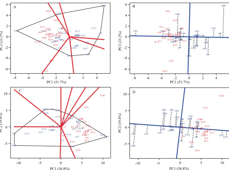
In the AMMI2 model (Figure 1 A), the genotypes close to the origin of the axes are more stable than the most distant ones, since they contributed little to the interaction. Combinations of genotypes and environments with the principal components of the same signal have specific positive interactions, whereas
combinations of opposing signals have specific negative interactions. The clones that contributed the least to the GxE interaction were G2, G20, G21, G22, and G25; and the E3, E5, E16, E18, and E22 environments were the most stable, considering their positions were close to the origin, that is, they showed the lowest scores for the two axes of the interaction.
The G11, G18, G19, and G21 clones interacted positively with the E7, E17, E20, and E23 environments, because they showed similar signal scores. Using a similar interpretation, the G1, G9, G28, and G29 clones also had positive specific interaction with the E2, E4, E5, E6, E9, E13, E19, and E22 environments. A distinct lack of adaptation of the G30 clone to the E10
environment was observed in the two graphs (markers pointing in opposite directions).
In the AMMI1 biplot (Figure 1 B), the abscissa represents the main effects (average of genotypes), and the ordinate, the first axis of interaction (PC1). Therefore, genotypes with IPCA1 values close to zero have high stability in the test environments.
The G3, G4, G6, G10, G15, G17, G18, G20, G22, G22, G23, G25, G26, G28, and G30 clones showed productivity below the general average (92 Mg ha-1),
while the other genotypes presented productivity equal to or above the average. The environments with low productivity were E2, E3, E6, E8, E9, E11, E16, E19, E22, and E24, whereas the other ones presented productivity equal to or above average. The more stable clones and environments correspond to the points around zero, relative to the horizontal axis (PC1), and the clones and environments associated with low productivity are located to the left of the figure.
For TPH, the G2, G7, G12, G17, G21, G22, and G28 clones were found to be the least responsive to the GxE interaction and, consequently, the most stable ones, because they had the lowest values for the two axes of the interaction (Figure 1 C). The G8, G12, G13, G19, and G27 clones were the ones with the highest mean and stability, being more distant from the abscissa, which represents the main effects (mean of genotypes), and were closer to the ordinate, representing the first axis of interaction (Figure 1 D). Therefore, genotypes with PC1 values close to zero were considered of high stability in the test environments. It should be highlighted that the G13, G12, and G27 clones were the most productive and stable for both TSH and TPH, being possible to infer that these clones have the potential to be indicated for cultivation.
Environmental stability is of great importance, because it indicates the reliability of genotype ordering, in a given environment, in relation to the classification by the average of the studied environments (Oliveira et al., 2003; Guerra et al., 2009). The most unstable environments were E1, E4, E6, E10, E12, E17, E23, and E24, while E1, E4, E12, E17, and E23 presented instability associated with high productivity.
Regarding productive performance, the genotype positioned at the vertex of the polygon is further distanced from the origin than all the genotypes within the sector delimited by it, being classified as the most responsive. This genotype may be better or worse in
some or all environments, and can be used to identify possible mega-environments. The genotypes located within the polygon were the least responsive to the stimuli of the environments (Figure 2 A and C).
Therefore, the environments grouped within this space had similar effect on the genotypes. For TCH and TPH, there was only one environmental grouping. For both variables, the G13 clone, located at the vertex of the polygon in the mega-environment, was the most favorable for this group of environments, with the highest yield in at least one of the environments and standing out as one of the genotypes with better performance in the other environments of the group.
The G3, G4, G18, G29, and G30 clones generated the other polygon vertices for both TSH and TPH, but no group of environments was formed within this sector comprising these clones, which were considered unfavorable to the groups of tested environments, with low productivity. Likewise, the clones located within the sectors delimited by them were also unfavorable for recommendation.
The most productive clone was G13, followed by G12, G5, and G27 for TSH (Figure 2 A). The least productive were: G30, G3, and G15 for TSH; and G3, G15, and G30 for TPH, because were located further away in the opposite direction.
The less stable clones were those with greater distances from the horizontal axis. Therefore, G30, G29, and G18 for TSH and G30, G29, G23, G4, and G18 for TPH were, in decreasing order, the most unstable. Considering the two evaluated parameters at the same time, the clones recommended due to high productivity value, good adaptability, and good stability were, in decreasing order, G13 and G12 for both variables.
Figure 2. Genotype main effects + genotype x environment interaction (GGE) biplot, representing tons of stem per hectare (TSH) (A) and tons of pol per hectare (TPH) (C), as well as averages x stability, indicating the productivity ranking for TSH (B) and TPH (D) of 30 sugarcane (Saccharum officinarum) clones evaluated in 24 environments (E) in 2014 and 2015. PC, principal components.
Conclusions
1. The G13 sugarcane (Saccharum officinarum) clone is highly productive in favorable and unfavorable environments, presenting the highest averages for ton of stems and pol per hectare.
2. The most promising clones for stability and general adaptability are G5, G12, and G13, according to the bisegmented regression method, to the additive main effects and multiplicative interaction analysis (AMMI), and to the genotype main effects + genotype x environment interaction (GGE biplot).
3. The G12 and G13 clones are the closest to the ideal genotype.
4. The G3, G4, G10, G15, G17, G18, G22, G23, G25, G26, and G30 clones are not recommended for the evaluated environments.
Acknowledgments
To Monsanto do Brasil Ltda., for support; and to Coordenação de Aperfeiçoamento de Pessoal de Nível Superior (Capes, process No. 184847-2), for scholarship granted.
References
ALBRECHT, J.C.; VIEIRA, E.A.; SILVA, M.S. e; ANDRADE, J.M.V. de; SCHEEREN, P.L.; TRINDADE, M. da G.; SOARES SOBRINHO, J.; SOUSA, C.N.A. de; REIS, W.P.; RIBEIRO JÚNIOR, W.Q.; FRONZA, V.; CARGNIN, A.; YAMANAKA, C.H. Adaptabilidade e estabilidade de genótipos de trigo irrigado no Cerrado do Brasil Central. Pesquisa Agropecuária Brasileira, v.42, p.1727-1734, 2007. DOI: 10.1590/S0100-204X2007001200009.
ANTUNES, W.R.; SCHÖFFEL, E.R.; SILVA, S.D. dos A. e; EICHOLZ, E.; HÄRTER, A. Adaptabilidade e estabilidade fenotípica de clones de canadeaçúcar. Pesquisa Agropecuária Brasileira, v.51, p.142-148, 2016. DOI: 10.1590/S0100-204X2016000200006.
CHEN, X.; JACKSON, P.; SHEN, W.; DENG, H.; FAN, Y.; LI, Q.; HU, F.; WEI, X.; LIU, J. Genotype × environment interactions in sugarcane between China and Australia. Crop and Pasture Science, v.63, p.459-466, 2012. DOI: 10.1071/CP12113.
CROSSA, J.; CORNELIUS, P.L. Sites regression and shifted multiplicative model clustering of cultivar trial sites under heterogeneity of error variances. Crop Science, v.37, p.406-415, 1997. DOI: 10.2135/cropsci1997.0011183X003700020017x. CRUZ, C.D.; REGAZZI, A.J.; CARNEIRO, P.C.S. Modelos biométricos aplicados ao melhoramento genético. 4.ed. Viçosa: Ed. da UFV, 2012. v.1, 514p.
CRUZ, C.D.; TORRES, R.A.; VENCOVSKY, R. An alternative approach to the stability analysis proposed by Silva and Barreto. Revista Brasileira de Genética, v.12, p.567-580, 1989.
DOMINGUES, L. da S.; RIBEIRO, N.D.; MINETTO, C.; SOUZA, J.F. de; ANTUNES, I.F. Metodologias de análise de
adaptabilidade e de estabilidade para a identificação de linhagens
de feijão promissoras para o cultivo no Rio Grande do Sul. Semina: Ciências Agrárias, v.34, p.1065-1076, 2013. DOI: 10.5433/1679-0359.2013v34n3p1065.
DUARTE, J.B.; VENKOVSKY, R. Interação genótipos x ambientes: uma introdução à análise “AMMI”. Ribeirão Preto:
Sociedade Brasileira de Genética, 1999. 60p. (Série Monografias,
n.9).
FERNANDES JÚNIOR, A.R.; ANDRADE, J.A. da C.; SANTOS, P.C. dos; HOFFMANN, H.P; CHAPOLA, R.G.; CARNEIRO, M.S.; CURSI, D.E. Adaptabilidade e estabilidade de clones de cana-de-açúcar. Bragantia, v.72, p.208-216, 2013. DOI: 10.1590/ brag.2013.033.
GABRIEL, K.R. The biplot graphic display of matrices with application to principal component analysis. Biometrika, v.58, p.453-467, 1971. DOI: 10.2307/2334381.
GARBUGLIO, D.D.; GERAGE, A.C.; ARAÚJO, P.M. de; FONSECA JUNIOR, N. da S.; SHIOGA, P.S. Análise de fatores
e regressão bissegmentada em estudos de estratificação ambiental
e adaptabilidade em milho. Pesquisa Agropecuária Brasileira, v.42, p.183-191, 2007. DOI: 10.1590/S0100-204X2007000200006. GUERRA, E.P.; OLIVEIRA, R.A. de; DAROS, E.; ZAMBON, J.L.C.; IDO, O.T.; BESPALHOK FILHO, J.C. Stability and adaptability of early maturing sugarcane clones by AMMI analysis. Crop Breeding and Applied Biotechnology, v.9, p.260-267, 2009. DOI: 10.12702/1984-7033.v09n03a08.
KUMAR, S.; HASAN, S.S.; SINGH, P.K.; PANDEY, D.K.; SINGH, J. Interpreting the effects of genotype × environment interaction on cane and sugar yields in sugarcane based on the AMMI model. Indian Journal of Genetics and Plant Breeding, v.69, p.225-231, 2009.
MIRANDA, G.C.; VIEIRA, C.; CRUZ, C.D.; ARAÚJO, G.A. de A. Comparação de métodos de avaliação da adaptabilidade e da estabilidade de cultivares de feijoeiro. Acta Scientiarum Agronomy, v.20, p.249-255, 1998. DOI: 10.4025/actasciagron. v20i0.4363.
OECD-FAO Agricultural Outlook 2015-2024. Paris: OECD; [Rome]: FAO, 2015. DOI: 10.1787/agr_outlook-2015-en.
OLIVEIRA, A.B. de; DUARTE, J.B.; PINHEIRO, J.B. Emprego da análise AMMI na avaliação da estabilidade produtiva em soja. Pesquisa Agropecuária Brasileira, v.38, p.357-364, 2003. DOI: 10.1590/S0100-204X2003000300004.
R CORE TEAM. R: a language and environment for statistical computing. Vienna: R Foundation for Statistical Computing, 2014. RAMALHO, M.A.P.; FERREIRA, D.F.; OLIVEIRA, A.C. de. Experimentação em genética e melhoramento de plantas. 3.ed. Lavras: Ed. da UFLA, 2012. 328p.
estabilidade de clones de cana-de-açúcar no estado de Minas Gerais. Ciência Rural, v.42, p.587-593, 2012. DOI: 10.1590/ S0103-84782012000400002.
VERISSIMO, M.A.A.; SILVA, S. dos A. e; AIRES, R.F.; DAROS, E.; PANZIERA, W. Adaptabilidade e estabilidade de genótipos precoces de cana-de-açúcar no Rio Grande do Sul. Pesquisa Agropecuária Brasileira, v.47, p.561-568, 2012. DOI: 10.1590/ S0100-204X2012000400012.
YAN, W.; HUNT, L.A.; SHENG, Q.; SZLAVNICS, Z. Cultivar evaluation and mega-environment investigation based on the GGE Biplot. Crop Science, v.40, p.597-605, 2000. DOI: 10.2135/ cropsci2000.403597x.
ZOBEL, R.W.; WRIGHT, M.J.; GAUCH JR., H.G. Statistical analysis of a yield trial. Agronomy Journal, v.80, p.388-393, 1988. DOI: 10.2134/agronj1988.00021962008000030002x.