Model
—
Modelling and Simulation
—Ivo Inácio Gomes
Thesis submitted as partial requirement for the degree of Master in Economics
Supervisor: Professor Vivaldo Mendes
Departament of Economics, ISCTE-IUL
Resumo
O dinheiro de helicóptero é um tema extremamente controverso que tem mere-cido muita atenção no decorrer dos últimos 5 anos. Nesta dissertação irei desenvolver um modelo DSGE que procura explicar como é que esta forma particular de criação de moeda poderá afectar a in‡ação e o hiato do produto. O modelo apresentado caracteriza o dinheiro de helicóptero como oferta de moeda permanente e explora as consequências do banco central restringir a sua capacidade de seguir uma polit-ica monetária mais restritiva no futuro, aumentando a quantidade de dinheiro de helicóptero presente na economia. Os factores mais relevantes que explicam o com-portamento do hiato do produto e da in‡ação são o efeito desta restrição na formação de expectativas de in‡ação e de consumo futuros.
Os resultados indicam que, para que o dinheiro de helicóptero seja considerado uma medida viável, o impacto da restrição da taxa de juro nas expectativas de consumo futuro precisa de ser grande o su…ciente para contrabalançar o efeito de aumento da expetativa de in‡ação futura.
Palavras-chave
Politica monetária, Modelos DSGE, "Dinheiro de helicóptero", Macroeconomia.
Classi…cação JEL
Abstract
Helicopter money is an extremely controversial topic that has been gaining a lot of attention over the last …ve years or so. In this dissertation I will develop a DSGE model that attempts to explain how this particular form of money creation may a¤ect in‡ation and the output gap. The model presented here characterizes helicopter money as permanent money supply and exploits the consequences of the central bank constraining its capacity to tighten monetary policy in the future by choosing a contemporaneous increase in helicopter money. The main factors behind the behavior of the output gap and in‡ation are explained by the impact of this constraint upon the formation of future in‡ation and consumption expectations. The results lead us to the conclusion that for helicopter money to be considered as a viable policy option, the impact of the interest rate constraint on expected future consumption needs to be high enough so that it counter-balances its e¤ect on expected future in‡ation.
Key-words
Monetary policy, DSGE models, Helicopter Money, Macroeconomics.
JEL Classi…cation
1 Introduction 1
2 Literature Review 3
2.1 Brief history of the idea . . . 3
2.2 De…nitions . . . 4
2.3 Di¤erent implementations . . . 4
2.4 Helicopter money vs QE . . . 5
2.5 Arguments in favor of helicopter money . . . 7
2.6 Critics . . . 11
3 Modelling and simulation 13 3.1 Household’s problem . . . 15
3.2 Firm’s problem . . . 18
3.3 The equilibrium . . . 20
3.4 Numerical Simulation . . . 23
3.4.1 Shocks in helicopter money . . . 23
3.4.2 Money supply shock . . . 26 v
3.4.3 Shocks in demand and supply . . . 27 3.5 Concluding Remarks . . . 29 References 31 Appendices 32 A Matlab code 33 B Figures: IRF 41
Introduction
Helicopter money is a controversial topic that has been gaining a lot of attention in the latest years. In the last few years, central banks have found their conven-tional tools used to conduct monetary policy to be ine¤ective, since interest rates e¤ectively reached the zero lower boundary (ZLB). Since then they have turned to more unconventional tools like quantitative easing programs, increasing central banks’balance sheets, although mostly with the public assurance that the purchases would eventually be reversed. Even though central banks used their biggest guns, they are still struggling in making monetary policy stimulate the economy. On the other side, …scal authorities are facing high levels of debt that are not compatible with a strong …scal stimulus, due to debt sustainability concerns. In the last years, helicopter money has surged as an idea that can potentially solve the problems of both …scal and monetary authorities, through cooperation between the two.
In this paper will build and analyze a model which looks at helicopter money and the impact it has in main economic variables, such as output gap and in‡ation. Even though helicopter money involves a level of cooperation between …scal and monetary
authorities, I chose to abstract from the …scal authority’s role in delivering a …scal stimulus to the economy. Instead I will focus my analysis on the main characteristic that distinguishes helicopter money from quantitative easing. While quantitative easing is designed to be temporary, helicopter money is a permanent stimulus. For this reason, the model treats helicopter money as permanent money supply.
This thesis is structured in 4 sections. Section 2 presents a literature review of the topic. Section 3 presents the model and section 4 presents an analysis of the model. In the end, section 5 concludes.
Literature Review
Since the …nancial crisis of 2008, central banks like the FED and the ECB have been struggling with a situation that have only been experienced in Japan in the last two decades. Central banks dropped interest rates to zero and bellow, recurring to quantitative easing programs (QE) to stimulate their economies when conven-tional monetary policy became depleted, and central banks’balance sheets grew to unprecedented values while in‡ation remained bellow target and the economy bellow potential. With this apparent lack of ability of monetary policy to stimulate the economy there has been increasing support for even more unconventional policies, like helicopter money. In this chapter I will look at the debate in the literature surrounding the implications of central banks’usage of helicopter drops as a part of their toolkit and what are the main arguments of its proponents and contestants.
2.1
Brief history of the idea
Helicopter money is an idea popularized by Milton Friedman in his paper “The Optimum Quantity of Money”published in 1969. In that paper, Friedman proposed
a thought experiment which consisted of dropping $1000 to an economy from a helicopter, to illustrate the costs of holding money as well as to demonstrate an e¤ortless way for the central bank to generate in‡ation if it wishes to (Friedman, 1969).
In the early 2000’s, this concept was brought back by the former federal reserve chairman Ben Bernanke regarding Japan’s liquidity trap, as one of several tools BoJ could use to bring back in‡ation to its desired level (Bernanke, 2000, 2003).
2.2
De…nitions
According to Ben Bernanke “a ‘helicopter drop’of money is an expansionary …scal policy – an increase in public spending or tax cut – …nanced by money creation” (Bernanke, 2016). In its essence is …scal policy …nanced by money creation. Another de…nition is given by Adair Turner, who says that "[m]onetary …nance is de…ned as running a …scal de…cit (or a higher de…cit than would otherwise be the case) which is not …nanced by the issue of interest-bearing debt, but by an increase in the monetary base – i.e. of the irredeemable …at non-interest-bearing monetary liabilities of the government/central bank."(Turner, 2015)
2.3
Di¤erent implementations
There are some ways helicopter money could be implemented. The central bank could transfer directly money to the government account, it could buy government bonds and transform them in perpetuities (with no principal nor interest payment). Central bank could also buy government debt and commit to its rolling over
per-petually and return the interest earned to the treasury as a pro…t, which simply means a perpetual QE (Nathan, 2017). It could also take the form of a permanent transfer from the central bank to households (people’s QE).
2.4
Helicopter money vs QE
To fully understand what helicopter money is and what alternative it provides, we need to understand the main di¤erences between this policy and other policies central banks have at their disposal. One policy that has been used largely all over the world recently is quantitative easing. It can be argued that QE can …nance an expansionary …scal policy. If the central bank decides to buy government bonds, it increases the monetary base and lowers the …nancing cost of public debt, allowing for the government to issue more debt to increase spending or cut taxes. The main issue with QE is that it is reversible, which means that the central bank will eventually drop the assets purchased back into the economy, reducing the monetary base and reverting the previous stimulus. If the principle of Ricardian Equivalence holds, economic agents’reaction may o¤set the stimulus. This reversibility does not happen with helicopter money, because it is a permanent measure. The fact that QE is temporary has two important consequences. Let’s consider a situation where the central bank buys government bonds in a QE operation. First, in a situation where …scal policy is constrained by sovereign debt default risk, a temporary purchase of government bonds does not reduce the debt sustainability problem. Although it reduces the government debt held by the private sector in the short run, in the long run the situation does not change, thus the government’s ability to pursue an
Figure 2.1: Money supply, monetary base and excess reserves in the US
expansionary …scal policy does not increase if it was limited by debt sustainability concerns. Second, if the increase of the monetary base is perceived by the economic agents as a temporary one, the impact on the money supply may be limited, as …gure 2.1 shows. Since the end of 2008, when the QE1 was used by the FED, monetary base increased four times, while money remained growing at roughly the same rate as before. However, the excess reserves of depository institutions held by the FED increased dramatically, which points to the fact that the stimulus did not have the e¤ect that was intended.
A permanent purchase of government bonds by the central bank funded by money creation, would permanently decrease the level of public debt held by the private sector as well as increase permanently monetary base.
2.5
Arguments in favor of helicopter money
Why do we need helicopter money? One argument in favor is linked with the idea of a balance sheet recession.
If the economy is in a situation where the private sector is deleveraging (balance sheet recession), monetary policy may not have the power to stimulate the economy. Richard Koo (2011) argues that when an economy is in a balance sheet recession (after a prolonged period of debt accumulation, the private sector is forced to clean its balance sheets), conventional monetary policy becomes ine¤ective, since “people with negative equity are not interested in increasing borrowing at any interest rate” (Koo, 2011: 20). The usual credit channel central banks use to …ght recessions doesn’t work, and debt minimization becomes more important to private agents with balance sheet problems than pro…t maximization. There is then a need for …scal policy to step in and do monetary policy’s work, while the private sector is deleveraging, to avoid a prolonged recession (Koo, 2011).
Adair Turner argues that the main issue of helicopter money is not technical, but political. His main concern is whether we can create mechanisms to ensure that monetary …nance is only use when appropriate. Turner also argues that debt …nance e¤ectiveness depends on whether Ricardian Equivalence holds or not in the real economy. Helicopter money on the other hand, does not need Ricardian agents to in‡uence consumers’ decision to spend, since there is no reason to be expected higher taxes in the future to o¤set the present stimulus (Turner, 2015).
money. They claim that there is a need to combine monetary with …scal stimu-lus (helicopter money), to help the government maintaining the stimustimu-lus while the deleveraging process occurs. Fiscal policy in this situation is very e¤ective, but is politically constrained due to fear of sovereign debt problems, so the stimulus provided by the …scal authority alone may be limited. A possible solution to each one of these two authorities’ problems could be …scal-monetary cooperation. On one hand, monetary policy solves the problem of lack of borrowing by substituting private with public borrowing. On the other hand, the …scal policy’s problem of excessive debt can be solved by monetizing some of it (McCulley & Pozsar, 2013).
This …scal-monetary cooperation allows for a simultaneous private sector delever-aging and an increase in nominal demand. Though one can be uncertain about how monetary …nance a¤ects separately real variables and the price level, Willem Buiter argues that it will always boost aggregate demand, either by increasing real output or in‡ation (or some combination of the two), given three conditions are met. The price of money must be positive, …at base money needs to have value other than its return and to be irredeemable (which means that is not considered as a liability by the central bank). This last condition is key to Buiter’s result, and in his partial equilibrium model it is represented by applying a solvency constraint on terminal non-monetary liabilities of the State (Government and Central Bank), instead of using …nancial liabilities as usual (Buiter, 2014).
“UK currency notes [. . . ] carry the proud inscription “promise to pay the bearer the sum of £ X” but this merely means that the Bank of England will pay out the face value of any genuine Bank of England note no matter how old. [. . . ] Because
it promises only money in exchange for money, this ‘promise to pay’ is [. . . ] a statement of the irredeemable nature of Bank of England notes.” (Buiter, 2014)
Ben Bernanke, who has earned the nickname of ‘Helicopter Ben’, has defended some form of helicopter money for Japan in some speeches (Bernanke, 2000) and (Bernanke, 2003), as a policy to increase nominal demand and get Japan out of the liquidity trap it su¤ers since the 1990’s. In a 2016 blog post (Bernanke, 2016), Bernanke argues that, though it is not likely that helicopter money will be used in the US in the short run, “under certain extreme circumstances— sharply de…cient aggregate demand, exhausted monetary policy, and unwillingness of the legislature to use debt-…nanced …scal policies— such programs may be the best available altern-ative. It would be premature to rule them out.” (Bernanke, 2016)
Kemal Dervis, former minister of Economic A¤airs of Turkey, points out the positive e¤ects of having the central bank printing money and bypassing the …nancial and corporate sectors and to deliver it straight into the middle and lower income consumers (Dervis, 2016). He argues that this would help to improve inclusiveness in economies with strong inequalities. Also, he claims that “Zero or negative real interest rates, when they become quasi-permanent, undermine the e¢ cient allocation of capital and set the stage for bubbles, bursts and crisis” (Dervis, 2016).
Because of the irredeemable feature of base money, we know that helicopter money will increase nominal demand. This is an important result, as it puts aside the hypothesis that de‡ation or secular stagnation are scenarios that an economy could get stuck in, regardless of the policies (monetary and …scal) pursued. Instead, they are policy choices (Buiter, 2014). The term of ‘helicopter money’was coined by
Milton Friedman in (Friedman, 1969), as a parable to demonstrate that there is no need for de‡ation since, if needed, the central bank could always drop money from a helicopter to the economy, and prices would eventually rise. However, is important to know how this increase in nominal demand is revealed in the economy. Either prices rise, output rises, or a combination of both will happen.
Jordi Galí tries to model the e¤ects on real variables as well as on the price level, of a …scal stimulus (increased government spending) …nanced with helicopter money, as opposed to the usual debt …nanced stimulus. (Galí, 2014) He compares a …scal stimulus in a Classical Monetary Model and in a New Keynesian Model, to …nd out that nominal rigidities are very important to explain the e¤ects of monetary …nance on output and in‡ation.
A …scal stimulus can be done in two separate ways, either by an increase in government spending, or by a tax cut. It is likely the e¤ects of monetary …nance of both kinds of policies will be di¤erent. The paper (Galí, 2014) was revised in December 2016, to include the e¤ects of both a tax cut and a government spending increase. It also analyzes a situation where the zero lower bound constraint (ZLB) on the nominal rate is binding. The results point out that helicopter money can help increasing output if there are su¢ cient nominal rigidities, only at the cost of relatively mild in‡ation. In the case of a binding ZLB, the way of …nancing appears to be less important (Galí, 2016).
2.6
Critics
However, such an unconventional idea has received also lots of criticism. Kocher-lakota defends that …nancing a government stimulus with debt or new money will end up having the same impact on the economy (Kocherlakota, 2016). Because central banks pay interest on reserves, any new money created would eventually have the same cost as if the …scal authority borrowed it. So, he argues, there is no need for helicopter money.
In my opinion Kocherlakota’s argument hinges on the assumption that the gov-ernment can sell bonds at an equal rate as the central bank deposit rate. This means that private agents don’t believe in a sovereign debt default, and see it as a safe asset. In this situation, the problem that …scal policy faces that requires the cooperation of monetary policy (McCulley & Pozsar, 2013) would no longer exist. The government could use …scal policy to stimulate the economy and gen-erate in‡ation (with a passive response by the central bank), without the need for help from monetary policy. However, Kocherlakota’s argument is well in noting that money has a cost too, not just debt. In a situation where the government is considered credible and no risk premium is charged on public debt, increasing base money would end up increasing reserves at the central bank, and the interest the government would save in bonds would be o¤set by less dividends from the central bank. However, this argument does not hold in a world where …scal authorities face credibility problems when public debt gets too high, thus losing power to stimulate the economy by themselves. In the case of public debt crisis, governments may face
positive risk premiums, which makes it e¤ectively cheaper for the central bank to create money instead of the …scal authority issuing bonds (helicopter money is not cost-free though, just a cheaper option in this case).
Claudio Borio et al. claim that embarking on helicopter money means to give up entirely on monetary policy. The basis of the argument rests on the lack of consideration for realistic interest rates by the central banks (Borio, Disyatat, & Zabai, 2016).
If a central bank decides to engage in monetary …nance, what are the con-sequences for its balance sheet? It ultimately depends on which way the central bank decides to it. If the central bank decides to buy government bonds and com-mits to roll them over perpetually, there would be an expansion of the central bank balance sheet (increase in government bonds and base money). If the central bank decides to write down public debt, replace it with non interest bearing perpetuities (which have a value of 0) or just transfer new money to individuals, it would have a negative impact on central bank equity.
Modelling and simulation
In this chapter I will describe the features and assumptions of the model economy. It is a new Keynesian DSGE model with Calvo pricing featuring helicopter money. In this framework, helicopter money is de…ned as the amount of money in the economy that is permanent. Let’s assume that the model economy has a single nominal interest rate which is controlled by the central bank by changing the amount of monetary base supplied to the economy. To simplify matters, assume that there is no intermediate banking, so that the monetary base is equal to money supply. To increase the quantity of money in circulation and reduce the nominal interest rate the central bank purchases riskless bonds from the household sector. By selling bonds back to the households the central bank reduces money supply and therefore raises interest rates. However, in this last case, the central bank may …nd itself without bonds left in its balance sheet to sell, becoming unable to decrease the quantity of money and increase the interest rate any further. Let’s assume a money demand function,
mt= yt rt (3.1)
where mt is the natural log of real money demand, yt represents the natural log of
real output, rtis the nominal interest rate and > 0 represents the semi-elasticity of
money demand. Let’s de…ne Htas helicopter money. Instead of being considered an
expansionary …scal policy …nanced by money creation, as Bernanke (2016) de…nes it, helicopter money will take other meaning in this model. In this framework, heli-copter money is de…ned as the minimum amount of money in circulation the central bank can achieve by selling bonds in its balance sheet. An increase in helicopter money can be interpreted has a giveaway of money to the economy, without re-sorting to the trade of bonds. However, a simple increase in helicopter money will not lead to an increase in money supply, which would continue to be dependent on equation (3.1).
Let’s de…ne rt as the maximum interest rate the central bank can achieve. From
equation (3.1) we get the maximum interest rate
rt =
1
(yt ht) (3.2)
where ht ln Ht. From the equation above we can see that helicopter money has
the e¤ect of limiting monetary policy by restricting the interest rate the central bank can set. Even though the central bank sets both the interest rate (following a Taylor rule) and helicopter money, these are two di¤erent instruments of monetary policy. While the former aims at keeping output gap and in‡ation close to a target level the latter can be thought of as a self-induced constraint on future (restrictive)
monetary policy. As a measure of the importance of this self-induced constraint, we
have t. Let’s de…ne t as
t rt rt; 0 (3.3)
where t describes how close the central bank is to become unable to raise interest
rates any further (a lower t means a more constrained central bank).
Using equations (3.1) and (3.2) we can describe the constraint using money supply and helicopter money.
t =
1
(mt ht) (3.4)
3.1
Household’s problem
The representative in…nitively-lived household maximizes the following intertem-poral utility function:
max Ut= Et 1 X i=0 t+k u(Ct+k; Nt+k) (3.5)
where Ct is the quantity of the single good consumed, Nt is the number of hours
worked and is the gross rate of intertemporal discount of utility.
The representative household then allocates her consumption between a set of consumption goods given by:
Ct Z 1 0 Ct(i)1 1 di 1 (3.6)
The representative household faces a period budget constraint of:
Z 1
0
Pt(i)Ct(i)di + QtBt= Bt 1+ WtNt (3.7)
where Pt is the price of the consumption good, Bt represents one-period riskless
bonds, bought in period t and maturing in t + 1. Qt is the price of a bond, which
gives 1 unit of money at maturity and Wt represents the nominal wage.
To avoid a situation where the household enters in a Ponzi-scheme, a solvency constraint is needed:
lim
T !1EtfBTg 0 (3.8)
Each good (i) faces a demand given by the following demand function
Ct(i) =
Pt(i) Pt
Ct (3.9)
where the price level is given by following equation.
Pt Z 1 0 Pt(i)1 di 1 1 (3.10) The aggregate nominal consumption is given by the equation below.
Z 1
0
Pt(i)Ct(i)di = PtCt (3.11)
From equations (3.7) and (3.11) we get the budget constraint for the represent-ative household below.
PtCt+ QtBt = Bt 1+ WtNt (3.12) Assuming a period utility function
u(Ct; Nt) Ct1 1
Nt1+'
1 + ' we get the following optimality conditions
wt pt= ct+ 'nt (3.13)
ct= Etct+1 1
(rt Et t+1 ) (3.14)
where lower case letters represent the natural log of the of corresponding upper case
letter (i.e. wt log Wt), and the nominal interest rate and household’s discount
rate are de…ned respectively as: rt log Q and log :
Now let’s assume that the interest rate constraint, given by t, has two
dif-ferent e¤ects on economic agents’ expectations. One a¤ects expectation of future consumption, and the other the expectations of future in‡ation. A higher constraint
(lower t), increases the probability of future interest rates being lower than
expec-ted in the case of a central bank not constrained. This e¤ect has a positive impact
on expected future consumption and is captured in the model by t, where
is the parameter that represents the future consumption e¤ect. The e¤ect on the expectations of future in‡ation, arises from the fear of monetary policy falling out of control of the central bank, since the central bank loses the ability to control
the model by 1! t;where ! is the parameter that represents the future in‡ation
e¤ect. Note that t and 1! t both have a positive impact on consumption,
when the constraint (and helicopter money) increases. These e¤ects lead to the Euler equation shown below.
ct = Etct+1 1 (rt Et t+1 ) 1 ! t t (3.15)
3.2
Firm’s problem
The …rms in the model economy set prices in a Calvo price setting . Each …rm has
a probability of not resetting its price each period. The optimal frictionless price
(pt) for …rms is achieved by each …rm wanting to charge a …xed markup ( ) over
the marginal cost mct(in logs), as stated in equation (3.18). The representative …rm
chooses it’s price to minimize the loss function (3.16).
L(zt) = 1 X k=0 ( )kEt(zt pt+k) 2 (3.16)
where zt is the price set by the proportion (1 )of …rms that reset their prices
in period t. zt= (1 ) 1 X k=0 ( )kEtpt+k (3.17) pt = + mct (3.18)
The price level in period t is given by the weighted average of the price level in
pt= pt 1+ (1 )zt (3.19)
Its also assumed that the real marginal cost ^mcrt is a function of real output yt,
with being the real output elasticity of real marginal costs.
^
mcrt = yt (3.20)
In‡ation ( t = pt pt 1) can then be written as equation (3.21), where xt is
the output gap and y represents the potential output level, which is set to zero for simplicity,
t= Et t+1+ xt (3.21)
where and xt are de…ned as
(1 )(1 )
(3.22)
xt yt y (3.23)
The e¤ect on the expectations of future in‡ation is also felt in equation (3.21),
and it is captured in the AS equation below as ! t.
3.3
The equilibrium
The goods market clearing condition is given the following condition.
yt = ct (3.25)
IS equation:
Putting together the Euler equation (3.15) and the goods market clearing condition
(equation 3.25) and adding a demand shock ut, we get the IS equation .
xt= Etxt+1 1 (rt Et t+1 ) ( ! + ) t+ ut (3.26) where ut= uut 1+ "ut; "ut (0; 1) AS equation:
To …nd the AS equation we only need to add a supply shock vt to (3.24)
t= Et t+1+ xt ! t+ vt (3.27)
where vt= vvt 1+ "vt; "vt (0; 1) Interest rate rule:
The central bank follows a Taylor rule in order to determine the nominal interest rate at any period t,
where and x are respectively the weight of in‡ation and output in the Taylor
rule, and x are the central bank’s in‡ation and output targets and rn is the
natural interest rate. Money demand
By adding a shock to the money demand (equation (3.1)), we get,
mt= yt rt+ st (3.29)
where st= sst 1+ "st; "st (0; 1) Helicopter money
The …nal assumption is that helicopter money follows an autoregressive process given by
ht= hht 1+ "ht (3.30)
where h is the persistence of the helicopter money shock and "ht a shock, .
Full model
By plugging equations (3.1) and (3.28) into equation (3.4) we get the expression below.
t =
1
((1 x)xt ht+ st) t (3.31)
a ! +
The next step is simply to insert the equations (3.28) and (3.31) into the IS and AS equations and add the four shocks and we get the full model.
Etxt+1+ 1 Et t+1 = (1 + x + a( 1 x))xt+ ( 1 a) t a ht ut+ a st (3.32) Et t+1 = [ + !( x 1 )]xt+ (1 ! ) t ! ht+ ! st vt (3.33) ht+1 = hht+ "ht+1 (3.34) ut+1 = uut+ "ut+1 (3.35) vt+1= vvt+ "vt+1 (3.36) st+1 = sst+ "st+1 (3.37)
3.4
Numerical Simulation
In this section I will simulate the behavior of the main variables of the model using impulse response functions (IRF’s) of each shock present for di¤erent parameters. The baseline calibration of the parameters can be seen in the Matlab routine used to generate the IRF’s that is available in Annex 1.
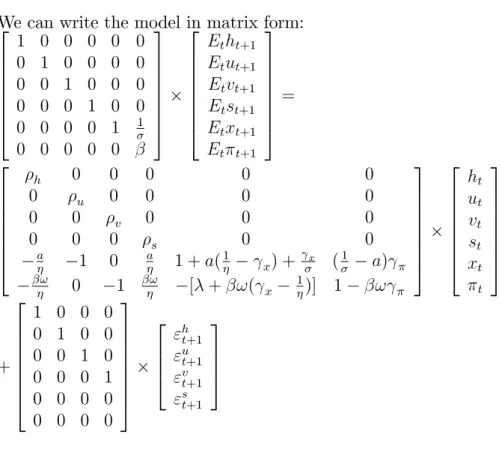
We can write the model in matrix form: 2 6 6 6 6 6 6 4 1 0 0 0 0 0 0 1 0 0 0 0 0 0 1 0 0 0 0 0 0 1 0 0 0 0 0 0 1 1 0 0 0 0 0 3 7 7 7 7 7 7 5 2 6 6 6 6 6 6 4 Etht+1 Etut+1 Etvt+1 Etst+1 Etxt+1 Et t+1 3 7 7 7 7 7 7 5 = 2 6 6 6 6 6 6 4 h 0 0 0 0 0 0 u 0 0 0 0 0 0 v 0 0 0 0 0 0 s 0 0 a 1 0 a 1 + a(1 x) + x (1 a) ! 0 1 ! [ + !( x 1)] 1 ! 3 7 7 7 7 7 7 5 2 6 6 6 6 6 6 4 ht ut vt st xt t 3 7 7 7 7 7 7 5 + 2 6 6 6 6 6 6 4 1 0 0 0 0 1 0 0 0 0 1 0 0 0 0 1 0 0 0 0 0 0 0 0 3 7 7 7 7 7 7 5 2 6 6 4 "ht+1 "u t+1 "v t+1 "st+1 3 7 7 5
3.4.1
Shocks in helicopter money
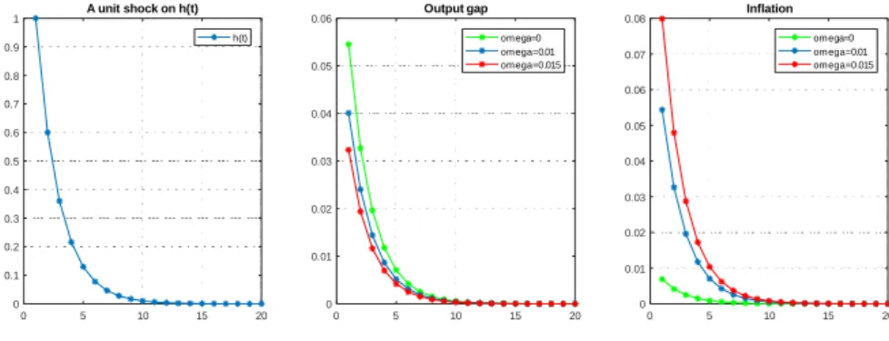
Figure 3.1 displays the IRF’s of a unit shock on ht, the helicopter money variable,
with a shock persistence h of 0:6 and = 0:02. Output and in‡ation both increase
with the shock. The …gure also shows how ! a¤ects the response of output gap and in‡ation. A higher !, would lead to a sharper response of in‡ation to helicopter
0 5 10 15 20 0 0.1 0.2 0.3 0.4 0.5 0.6 0.7 0.8 0.9 1 A unit shock on h(t) h(t) 0 5 10 15 20 0 0.01 0.02 0.03 0.04 0.05 0.06 Output gap omega=0 omega=0.01 omega=0.015 0 5 10 15 20 0 0.01 0.02 0.03 0.04 0.05 0.06 0.07 0.08 Inflation omega=0 omega=0.01 omega=0.015
Figure 3.1: IRF’s of a helicopter money shock ( = 0:02)
money and a smaller increase of output gap. This happens because the central bank is still setting interest rates and following a Taylor rule. Even though a higher expectation of in‡ation in the future as an e¤ect of increasing both output and in‡ation in the …rst place, the rise of the interest rate to control in‡ation o¤sets the positive e¤ect on output gap.
Figure 3.2 shows the impulse response functions of output gap and in‡ation, but
this time for di¤erent values for : As expected, output increases more if is higher.
If is su¢ ciently close to zero, a helicopter money shock decreases output gap. This
happens because of the impact of helicopter money on in‡ation, and the increase in the interest rate to o¤set it causes a downward pressure on output gap. This result points to the conclusion that for helicopter money to be considered a viable policy
option, needs to be high enough so that it counters the in‡ation e¤ect given by !.
The persistence of the shock is also a crucial factor in determining the e¤ects of a helicopter money shock. A higher persistence means that the central bank will keep itself constrained for longer after taking the policy decision of increasing
0 5 10 15 20 0 0.2 0.4 0.6 0.8 1 A unit shock on h(t) h(t) 0 5 10 15 20 -0.02 -0.01 0 0.01 0.02 0.03 0.04 0.05 Output gap k=0 k=0.01 k=0.02 0 5 10 15 20 0 0.01 0.02 0.03 0.04 0.05 0.06 Inflation k=0 k=0.01 k=0.02
Figure 3.2: IRF’s of a helicopter money shock (! = 1)
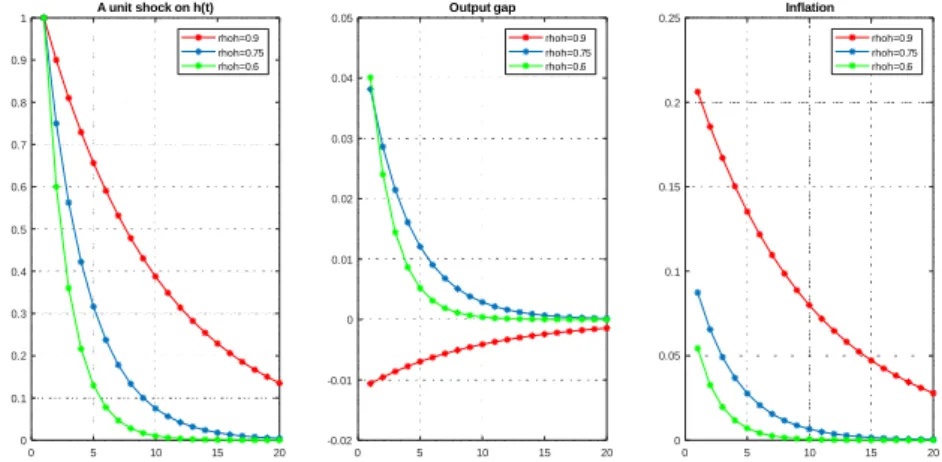
helicopter money. A low persistence on the other hand will mean that the constraint that helicopter money creates is phased out quicker. Figure 3.3 shows the impulse response functions of unit shocks on helicopter money with di¤erent persistences.
One can observe that a higher value for h leads to and increase in the response
of in‡ation, from a 0.05% increase in the …rst period with h = 0:6 to an increase
of 0.2% in the …rst period with h = 0:9; with the e¤ect on in‡ation persisting
even after 20 periods away from the shock. This e¤ect on in‡ation puts downward pressure on output gap when the persistence of the shock is high. The result can be
seen in the response of output to the shocks. For small values of h;an increase in
the persistence will lead to a higher increase in output gap in response to the shock.
However, after a certain threshold of h, the in‡ation pressure on interest rates of a
higher persistence gets high enough to fully o¤set the positive e¤ect. With h = 0:9
output gap even decreases 0.01% when subject to a unit shock of helicopter money.
A helicopter money shock with h = 0:6, apears to be more e¤ective at increasing
0 5 10 15 20 0 0.1 0.2 0.3 0.4 0.5 0.6 0.7 0.8 0.9 1 A unit shock on h(t) rhoh=0.9 rhoh=0.75 rhoh=0.6 0 5 10 15 20 -0.02 -0.01 0 0.01 0.02 0.03 0.04 0.05 Output gap rhoh=0.9 rhoh=0.75 rhoh=0.6 0 5 10 15 20 0 0.05 0.1 0.15 0.2 0.25 Inflation rhoh=0.9 rhoh=0.75 rhoh=0.6
Figure 3.3: IRF’s of a helicopter money shock (! = 0:01; = 0:02)
3.4.2
Money supply shock
We can see by looking at the …gure 3.4, that a positive shock in the money supply has the exact opposite e¤ect as a helicopter money shock, if the persistence of the shocks is equal. This could be explained by the fact that the channel through which money supply a¤ects the economy is the same as the one used by helicopter money. An increase in money supply e¤ectively reduces the interest rate constraint the central bank faces. This feature means that e¤ect of helicopter money in the model economy will depend on money supply shocks as well. Figure 3.4 show the IRF’s
of a unit shock in the money supply, with a persistence ( s) of 0:6, ! = 0:01 and
= 0:02:
This result points to the conclusion that for helicopter money to be considered
a viable policy option, needs to be high enough so that it counters the in‡ation
0 5 10 15 20 0 0.1 0.2 0.3 0.4 0.5 0.6 0.7 0.8 0.9 1 A unit shock on h(t) h(t) 0 5 10 15 20 -0.05 -0.04 -0.03 -0.02 -0.01 0 0.01 0.02 0.03 0.04 0.05 Output gap h shock s shock 0 5 10 15 20 -0.06 -0.04 -0.02 0 0.02 0.04 0.06 Inflation h shock s shock
Figure 3.4: Helicopter money and money supply shocks
3.4.3
Shocks in demand and supply
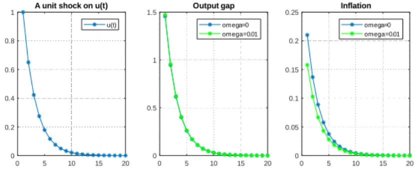
I will now analyze how changes in ! a¤ect shocks of demand (u) and supply (v).
With the baseline parameters (! = 0:01; = 0:02) and a unit demand shock with
a persistence ( u) of 0.65 increases output gap by 1.5% and in‡ation by 0.15% in
period 1, as …gure 3.5 shows. However, reducing ! has the e¤ect of a sharper increase in in‡ation in response to a demand shock, even with a similar response of output gap (see …gure 3.5). This might be an e¤ect of agents putting more weight (higher
!) on central bank’s control over monetary policy when forming future in‡ation
expectations. A higher value for ! would mean that although helicopter money shocks have worse e¤ects on in‡ation, business cycles caused by demand shocks would lead to more stable in‡ation.
A positive unit shock on the supply side (vtincreases) with = 0:02and ! = 0:01
and ! = 0 generates the IRF’s depicted in …gure 3.6. Output gap decreases by near 2% in period 1 while in‡ation increases in period 1 by 3%.
0 5 10 15 20 0 0.2 0.4 0.6 0.8
1 A unit shock on u(t)
u(t) 0 5 10 15 20 0 0.5 1 1.5 Output gap omega=0 omega=0.01 0 5 10 15 20 0 0.05 0.1 0.15 0.2 0.25 Inflation omega=0 omega=0.01
Figure 3.5: Demand shock ( = 0:02)
0 5 10 15 20 0 0.1 0.2 0.3 0.4 0.5 0.6 0.7 0.8 0.9 1 A unit shock on v(t) v(t) 0 5 10 15 20 -2 -1.8 -1.6 -1.4 -1.2 -1 -0.8 -0.6 -0.4 -0.2 0 Output gap omega=0 omega=0.01 0 5 10 15 20 0 0.5 1 1.5 2 2.5 3 3.5 Inflation omega=0 omega=0.01
3.5
Concluding Remarks
Helicopter money has becoming over the last …ve years one major monetary strategy (possibly) available to central banks and governments to combat long periods of economic stagnation. The fact that this strategy is not possible to be implemented from a legal point of view in most (if not all) advanced industrialized countries, does not mean that one should not enquire about its potentiality as an important new tool in monetary policy. I hope that this paper may shed some light in the huge discussions that have been taking place recently, by providing a simple framework in which helicopter money can be analyzed: the standard New Keynesian Model.
There is some relevant issues that we can clearly see from the model presented here. This model characterizes helicopter money as permanent money supply and exploits the consequences of the central bank constraining its capacity to tighten monetary policy in the future by choosing a contemporaneous increase in helicopter money. The main factors behind the behavior of the output gap and in‡ation are explained by the impact of this constraint upon the formation of future in‡ation and consumption expectations. The results lead us to the conclusion that for heli-copter money to be considered as a viable policy option, the impact of the interest rate constraint on expected future consumption needs to be high enough so that it counter-balances its e¤ect on expected future in‡ation.
Our model also seems to suggest that if private economic agents give a higher weight (or are more reactive) to helicopter money when forming their in‡ation ex-pectations, helicopter money will have more adverse e¤ects on the economy.
How-ever, the reaction of in‡ation to demand shocks becomes less sharp. This feature may give some support to the idea of keeping helicopter money away from the central bank’s policy arsenal even if it could be a useful strategy in some extreme situations. The e¤ect of stabilization of demand shocks, if economic agents become irrationally (or rationally) suspicious of helicopter money drops, can eventually over-come the drawback of not having the option available. However, a helicopter drop well planned by the central bank, announced to be phased out at the right rate may increase output at a mild cost of in‡ation.
One possible future development of the model would be to have the central bank operating at the zero lower bound, where it seems to be a better scenario to consider helicopter drops.
[1] Bernanke, B. S. (2000). Japanese Monetary Policy: A Case of Self-Induced Paralysis?, Princeton University , 1–27. Retrieved on September 15, 2017 from http://www.princeton.edu/~pkrugman/bernanke_paralysis.pdf
[2] Bernanke, B. S. (2003). Some Thoughts on Monetary Policy in Japan, speech before the Japan Society of Monetary Economics, Tokyo, Japan, 1–11.
[3] Bernanke, B. S. (2016). What tools does the Fed have left? Part
3: Helicopter money. Retrieved on September 15, 2017, from
https://www.brookings.edu/blog/ben-bernanke/2016/04/11/what-tools-does-the-fed-have-left-part-3-helicopter-money/
[4] Borio, C., Disyatat, P., & Zabai, A. (2016). Helicopter money: The illu-sion of a free lunch. Vox article, 1–5. Retrieved on September 15, 2017 from http://voxeu.org/article/helicopter-money-illusion-free-lunch
[5] Buiter, W. H. (2014). The simple analytics of helicopter money: Why it works - Always. Economics, 8(1), 0–52. Retrieved on September 15, 2017 from https://doi.org/10.5018/economics-ejournal.ja.2014-28
[6] Dervis, K. (2016). Time for Helicopter Money - Project
Syndic-ate, retrieved on 15 September 2017 from
https://www.project- syndicate.org/commentary/coordinated-monetary-policy-revive-growth-by-kemal-dervis-2016-03?
[7] Friedman, M. (1969). The optimum quantity of money. Transaction Publishers, New York
[8] Galí, J. (2014). The E¤ects of a Money-…nanced Fiscal Stimulus. Universitat Pompeu Fabra Economics Working Paper, (version September 2014).
[9] Galí, J. (2016). The E¤ects of a Money-Financed Fiscal Stimulus, mimeo, Uni-verssitat Ponpeu Fabra Working Paper (version December 2016)
[10] Kocherlakota, N. (2016). “Helicopter Money” Won’t Provide Much
Ex-tra Lift- Article from Bloomberg View, retrieved on September 15,
2017 from https://www.bloomberg.com/view/articles/2016-03-24/-helicopter-money-won-t-provide-much-extra-lift
[11] Koo, R. (2011). The world in balance sheet recession: causes, cure, and politics. Real World Economics Review, (58), 19–37.
[12] McCulley, P., & Pozsar, Z. (2013). Helicopter Money: Or How I Stopped Wor-rying and Love Fiscal-Monetary Cooperation. Global Interdependence Center Working Paper Series, 37.
[13] Nathan, A. (2017). Our Thinking - What’s Top of Mind
“Heli-copter Money”, Goldman Sachs, retrieved on September 15, 2017 from http://www.goldmansachs.com/our-thinking/pages/helicopter-money.html [14] Turner, A. (2015). The Case for Monetary Finance – An Essentially Political
Issue. 6th IMF Annual Research Conference, “Unconventional Monetary and Exchange Rate Polices,” 1–38
Matlab code
beta=0.99; sigma=2; rn=0.02; gama=0.6; theta=0.75; lambda=gama*(((1-theta)*(1-theta*beta))/theta); gamapi=1.5; gamax=0.5; pistar=0; xstar=0; eta=0.5; omega=0.01; k=0.02; a=(omega/sigma)+k; rhoh=0.6; 33rhou=0.65; rhov=0.7; rhos=0.75; A=zeros(6,6); A(1,1)=1; A(2,2)=1; A(3,3)=1; A(4,4)=1; A(5,5)=1; A(5,6)=1/sigma; A(6,6)=beta; B=zeros(6,6); B(1,1)=rhoh; B(2,2)=rhou; B(3,3)=rhov; B(4,4)=rhos; B(5,1)=-a/eta; B(5,2)=-1; B(5,4)=a/eta; B(5,5)=1+a*((1/eta)-gamax)+(gamax/sigma); B(5,6)=gamapi*((1/sigma)-a); B(6,1)=-beta*omega/eta; B(6,3)=-1;
B(6,4)=beta*omega/eta; B(6,5)=-(lambda+beta*omega*(gamax-1/eta)); B(6,6)=1-beta*omega*gamapi C=zeros(6,4); C(1,1)=1; C(2,2)=1; C(3,3)=1; C(4,4)=1 E=inv(A)*B F=inv(A)*C [vectors,eigenvalues]=eig(E) val=diag(eigenvalues) t=sortrows([val vectors’],1) eigenvalues=diag(t(:,1)) vectors=t(:,2:7)’ pstar=inv(vectors) LAMBDA1=eigenvalues(1:4,1:4) LAMBDA2=eigenvalues(5:6,5:6) P11=pstar(1:4,1:4) P12=pstar(1:4,5:6) P21=pstar(5:6,1:4) P22=pstar(5:6,5:6) R=pstar*F
D=P11-P12*inv(P22)*P21; f=-inv(P22)*P21 R1=R(1:4,:) g=inv(D)*R1 z=inv(D)*LAMBDA1*D n=20; irf_h=zeros(6,n); irf_u=zeros(6,n); irf_v=zeros(6,n); irf_s=zeros(6,n); irf_h(1:4,1)=g*[1;0;0;0]; irf_u(1:4,1)=g*[0;1;0;0]; irf_v(1:4,1)=g*[0;0;1;0]; irf_s(1:4,1)=g*[0;0;0;1]; i=1; for i=1:(n-1); irf_h(1:4,i+1)=z*irf_h(1:4,i); irf_u(1:4,i+1)=z*irf_u(1:4,i); irf_v(1:4,i+1)=z*irf_v(1:4,i); irf_s(1:4,i+1)=z*irf_s(1:4,i); end; irf_h(5:6,:)=f*irf_h(1:4,:); irf_u(5:6,:)=f*irf_u(1:4,:);
irf_v(5:6,:)=f*irf_v(1:4,:); irf_s(5:6,:)=f*irf_s(1:4,:); irf_h=real(irf_h); irf_u=real(irf_u); irf_v=real(irf_v); irf_s=real(irf_s); h_h=irf_h(1,:); u_h=irf_h(2,:); v_h=irf_h(3,:); s_h=irf_h(4,:); x_h=irf_h(5,:); pi_h=irf_h(6,:); …gure subplot(231);plot(h_h,’-*’); legend(’h(t)’); grid on; subplot(232);plot(u_h,’-*’); legend(’u(t)’); grid on; subplot(233);plot(v_h,’-*’); legend(’v(t)’); grid on; title(’A unit shock on h(t)’) subplot(234);plot(s_h,’-*’); legend(’s(t)’); grid on; subplot(235);plot(x_h,’-*’);
legend(’x(t)’); grid on; subplot(236);plot(pi_h,’-*’); legend(’pi(t)’); grid on; h_u=irf_u(1,:); u_u=irf_u(2,:); v_u=irf_u(3,:); s_u=irf_u(4,:); x_u=irf_u(5,:); pi_u=irf_u(6,:); …gure subplot(231);plot(h_u,’-*’); legend(’h(t)’); grid on; subplot(232);plot(u_u,’-*’); legend(’u(t)’); grid on; subplot(233);plot(v_u,’-*’); legend(’v(t)’); grid on; title(’A unit shock on u(t)’) subplot(234);plot(s_u,’-*’); legend(’s(t)’); grid on; subplot(235);plot(x_u,’-*’); legend(’x(t)’); grid on; subplot(236);plot(pi_u,’-*’); legend(’pi(t)’); grid on;
h_v=irf_v(1,:); u_v=irf_v(2,:); v_v=irf_v(3,:); s_v=irf_v(4,:); x_v=irf_v(5,:); pi_v=irf_v(6,:); …gure subplot(231);plot(h_v,’-*’); legend(’h(t)’); grid on; subplot(232);plot(u_v,’-*’); legend(’u(t)’); grid on; subplot(233);plot(v_v,’-*’); legend(’v(t)’); grid on; title(’A unit shock on v(t)’) subplot(234);plot(s_v,’-*’); legend(’s(t)’); grid on; subplot(235);plot(x_v,’-*’); legend(’x(t)’); grid on; subplot(236);plot(pi_v,’-*’); legend(’pi(t)’); grid on; h_s=irf_s(1,:);
u_s=irf_s(2,:); v_s=irf_s(3,:);
s_s=irf_s(4,:); x_s=irf_s(5,:); pi_s=irf_s(6,:); …gure
subplot(231);plot(h_s,’-*’); legend(’h(t)’); grid on; subplot(232);plot(u_s,’-*’); legend(’u(t)’); grid on; subplot(233);plot(v_s,’-*’); legend(’v(t)’); grid on; title(’A unit shock on s(t)’) subplot(234);plot(s_s,’-*’); legend(’s(t)’); grid on; subplot(235);plot(x_s,’-*’); legend(’x(t)’); grid on; subplot(236);plot(pi_s,’-*’); legend(’pi(t)’); grid on;
Figures: IRF
0 5 10 15 20 0 0.2 0.4 0.6 0.8 1 h(t) 0 5 10 15 20 0 1 2 3 4 5 10 -34 u(t) 0 5 10 15 20 0 1 2 3 4 10 -18A unit shock on h(t) v(t) 0 5 10 15 20 -1 -0.5 0 0.5 1 s(t) 0 5 10 15 20 0 0.005 0.01 0.015 0.02 0.025 0.03 x(t) 0 5 10 15 20 0 0.01 0.02 0.03 0.04 0.05 0.06 pi(t)
Figure B.1: IRF’s of a helicopter money shock (! = 0:01; = 0:02)
0 5 10 15 20 -1 -0.5 0 0.5 1 h(t) 0 5 10 15 20 -8 -6 -4 -2 0 10 -34 u(t) 0 5 10 15 20 -6 -5 -4 -3 -2 -1 0 10 -18A unit shock on s(t) v(t) 0 5 10 15 20 0 0.2 0.4 0.6 0.8 1 s(t) 0 5 10 15 20 -0.02 -0.015 -0.01 -0.005 0 x(t) 0 5 10 15 20 -0.1 -0.08 -0.06 -0.04 -0.02 0 pi(t)
0 5 10 15 20 -1 -0.5 0 0.5 1 h(t) 0 5 10 15 20 0 0.2 0.4 0.6 0.8 1 u(t) 0 5 10 15 20 0 0.5 1 1.5 2 2.5 3 10
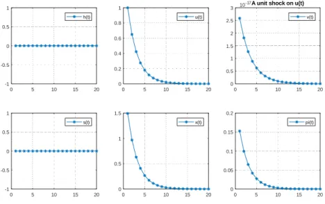
-17A unit shock on u(t) v(t) 0 5 10 15 20 -1 -0.5 0 0.5 1 s(t) 0 5 10 15 20 0 0.5 1 1.5 x(t) 0 5 10 15 20 0 0.05 0.1 0.15 0.2 pi(t)
Figure B.3: IRF’s of a demand shock (! = 0:01; = 0:02)
0 5 10 15 20 -1 -0.5 0 0.5 1 h(t) 0 5 10 15 20 0 0.2 0.4 0.6 0.8 1 10 -17 u(t) 0 5 10 15 20 0 0.2 0.4 0.6 0.8 1 A unit shock on v(t) v(t) 0 5 10 15 20 -1 -0.5 0 0.5 1 s(t) 0 5 10 15 20 -2.5 -2 -1.5 -1 -0.5 0 x(t) 0 5 10 15 20 0 1 2 3 4 pi(t)