Volume 1 Number 1, June 2012, Page 31-46
ISDS Article ID: IJDS12040401
A macro-econometric diagnosis of the
Keynesian propositions of the money
demand function in Malawi: An
error-correction approach
Ken Chamuva Shawa
*Catholic University of Eastern Africa, P.0. Box 62157, 00200, Nairobi, Kenya
Abstract
The institution of sound monetary policies largely depends on a good understanding of the money demand function. While there have been studies to understand the behaviour of the money demand function in general, critical analyses solely devoted to testing Keynesian propositions, particularly in developing countries, are rare. Using data from 1970 to 2005, the study employs the Augmented Dickey-Fuller (ADF) procedure to test for non-stationarity and the Johansen procedure to test for a long-run equilibrium relationship among economic fundamentals. Due to non-stationarity of variables an error-correction mechanism is used to characterise the money demand function in
Malawi. Although the income elasticity of money demand bears the expected positive sign, contrary to Keynes’
contentions, the study finds a stable demand function and an inelastic interest rate elasticity of money demand. The level of financial development and exchange rates are also found significant in influencing money demand in Malawi. Vital policy implications can be drawn from the results. First, monetary policy should be undertaken bearing in mind the stability of the money demand function and the less than proportionate response of money demand to interest rate changes. Second, policies to improve the functioning of the financial sector are indispensable. Nonetheless, such policies should be supported by prudent exchange rate management to check currency substitution.
Keywords:
Interest elasticity, Income elasticity, Motives of holding money, Cointegration
Copyright © 2012 ISDS LLC (JAPAN) - All Rights Reserved International Society for Development and Sustainability (ISDS)
Cite this paper as: Shawa, K.C. , A macro-econometric diagnosis of the Keynesian
propositions of the money demand function in Malawi: An error-correction approach , International
1.
Introduction
The demand for money function is at the heart of monetary policy. Demand for money can be defined as the demand for cash balances that individuals want to hold in the pocket. It is the demand for liquid or semi – liquid assets that can be easily used as a medium of exchange. Most Central Banks rely on the demand for money function as a means to identify medium-term growth targets for money supply. Indeed as noted by Treichel (1997), this function is also used to manipulate interest rates and the reserve money for the purpose of controlling total liquidity in the economy. Consequently, the importance of the stability of the money demand function is unquestionable. Unsurprisingly thus, Arrau et al. (1991) argue that an unstable demand function is likely to mar the predictable effect of both monetary and fiscal policies. To them, the demand for money is significant in assessing the welfare implications of policy changes and for determining the role of seignorage in an economy.
(owever, the argument on the stability of the money demand function contradicts Keynes’s contention, at least in the relative sense (Sloman, 1997). For Keynes, the demand for money is not a stable function and it is affected by an interest rate in a very elastic manner. He argues that the interest elasticity of demand for cash balances is greater than unity. This is because money is a store of wealth and that it is a close substitute to other financial assets.1
Literature documents many studies on demand for money. However, the study of Ball (1998) has been influential to many other studies. Ball investigated a long-run demand function for M1 in the Postwar United States. The study established an income elasticity of money demand of approximately 0.5 and the interest elasticity of approximately -0.05. In Africa, Treichel (1997) examined broad money demand and monetary policy in Tunisia. The study finds a stable money demand function. In Asia, Qayyum (2005) modelled the demand for money (M2) in Pakistan. The study finds inflation significant in the short run, while interest rate, market rate, and bond yield are important for the long-run money demand behaviour. This study employed cointegration analysis.
Other studies have generally concentrated on measures of uncertainty. For instance, Greiber and Lemke (2005), construct a measure of macroeconomic uncertainty from several observable economic indicators for the euro area. Cointegration results show that the extracted measures of uncertainty help explain the increase in euro area- M3 over the period 2001 and 2004 and the study by Arrau et al. (1991), finds that financial innovations play a significant role in the demand for money. These results were obtained from a model of demand for money in ten developing countries.
One can argue that although there have been many studies on money demand very few have specifically undertaken to assess the validity of Keynes’s propositions. The propositions have been generally accepted as applicable in both the developed and developing world, yet monetary policy is rooted in empirical foundations. As Sato (2001) rightly notes, the choice of money supply target is based on the function of money itself. This emphasises Treichel’s contention that the demand for money function is the function upon which Central Banks rely to identify medium-term growth targets for money supply and also to manipulate
interest rates and the reserve money for the purpose of controlling total liquidity in the economy. In the case of Malawi therefore, it is imperative to assess empirically whether the propositions about money demand hold. For particularity, the present study assesses the Keynesian propositions of money demand and explores the implications of the findings on the conduct of monetary policy in Malawi. It is glowingly clear that the results of this study will form a vital basis for the direction of the conduct of monetary policy in Malawi. Besides, to my knowledge, there has been no study interested in testing the Keynesian propositions of demand function for policy analysis in Malawi. Most studies have concentrated on general formulations of money demand.
The rest of the paper is organised as follows: Section 2 discusses the Keynesian propositions on money demand, section 3 discusses the methodology, section 4 discusses empirical results and section 5 presents the conclusions and direction for further research.
2.
Keynesian propositions of the money demand function
To Keynes people hold money primarily for three motives. He called the first motive, the transactions motive , the second, the precautionary motive , and the third the speculative motive .
2.1.
The transactions motive
The transactions motive is derived from the use of money as the medium of exchange. Economic agents access money only in intervals such as after a month, yet they require to conduct transactions at their convenience. Thus they must hold some cash balances, liquid enough for their day to day transactions. The demand for money for day to day transactions is called transactions demand .
This basic argument of Keynes was exposed to more rigorous work by Baumol (1952) and Tobin (1956). Baumol and Tobin analysed the behaviour of an individual transactor, be it a firm or a household. This individual transactor receives an income payment once per time period, say, per month. However, the transactor must spread out his purchases over time. The costs incurred by the transactor have two components: One comes from selling bonds where a brokerage fee must be paid. The other is the interest foregone if money is held instead of bonds. The total cost of making transactions,
can then be written as:2
K r K T b
(1)
It is argued that money holdings over the period have an average value of K/2, and the demand for money equation that emerges from this analysis is:
r bT K
P
Md 2
2 1
2
Equation 2 implies that is the demand for transactions balances measured in real terms is proportional to the square root of the volume of transactions and inversely proportional to the square root of the rate of interest. This can be rewritten as
5 . 0 5 . 0 5 . 0 2
2
1
p b T r
r bT
Md where 2
2 1
(3)
Thus Baumol’s approach to the demand for money implies that money is a means of exchange in the economy and that there is a cost in transforming interest-earning assets into money, a brokerage fee. If one substitutes zero for b in equation 3, the expression will clearly reduce to zero, telling us that, if no cost were involved in selling bonds, there would be no demand for money, even in an economy in which it is the only
means of exchange.
2.2.
The precautionary motive
In the Keynesian framework, the transactions demand for money is only part of the total demand. The precautionary motive is closely associated with it. Transactions-demand analysis deals with a demand for money that arises even when an individual’s pattern of income receipts and expenditure is given to him and known with perfect certainty; analysis of the precautionary motive is concerned with the impetus to money holding generated by uncertainty about the timing of cash inflows and outflows. In this regard, consider the behaviour of an individual whose income matches his expenditure, not on a period-by-period-let us say month-by month-basis, but only on average over a number of months. In any particular month, there may arise an excess or shortfall of income over expenditure. If there is an excess, it is added to his wealth, but a shortfall decreases his wealth. Thus in general the uncertainties about receipts and payments induce economic agents and firms to hold some precautionary balances (Laidler, 1997, 1999).
Therefore both the transactions demand and precautionary demand depend directly on the level of real income. Keynes summed the precautionary and transactions demand to form what has come to be known in economic circles as Liquidity Preference (the desire to hold money in liquid form). When money balances are held for the two purposes they are referred to as Active Balances (Sloman, 1997). The demand for active balances is positively related to income. Higher incomes induce more purchases which eventually increase demand for active balances or liquidity. Algebraically we represent the sum of demand for the two purposes in the following function
(mt mp) f y( )
(4)
2.3.
The speculative motive
The speculative demand for money arises because, unlike other financial assets, the capital value of money does not change with changes in the interest rate and because there is uncertainty about the manner in which the interest rate will change in the future. Keynes’s solution to such problems was to posit that as far as the choice between holding bonds and money is concerned, each individual acts as if he is certain about what is going to happen to the interest rate, and hence holds either bonds or money depending upon his expectations (Laidler, 1977, 1999).
Consequently the Demand for money is speculative when one considers putting money in some interest-bearing assets such as stocks and shares. The major determinant of speculative demand for money balances is the earning potential of securities and other assets (Sloman, 1997). An expectation of a boom in the stock market with rapid growth in share prices forces economic agents to switch some of their wealth into stocks and shares. The greater the earning potential of non-money assets, the less will be the demand for money. Individuals and firms will demand less money.
Generally, if the price of securities is high, the rate of interest on these securities will be low. Potential purchasers of these securities will probably wait until their prices fall and the rate of interest rises. Similarly existing holders of securities will probably sell them while the price is high, hoping to buy them back again when the price falls, thus making a capital gain. In the meantime, therefore, large speculative balances of money will be held, the speculative demand for money balances is high. If on the other hand the interest is high, then speculative demand will be low. To take advantage of the high rate of return on securities, people buy them now instead of holding on to their money.
We thus represent speculative demand as a decreasing function of the rate of interest as follows
(ms) f R( )
(5)
where
m
srepresents speculative demand, Rrepresents interest rate, and the minus sign emphasizes the inverse relationship.In summary therefore, according to Keynes, the demand for money is interest elastic and an unstable function of income and interest rate. It is represented as follows:
(md) f Y R( , )
(6)
3.
Methodology
The methodology used here is three-tier. It starts with, model specification for econometric analysis, then time series formulations are explained, and, finally an error correction model is estimated. The time series formulations include unit root tests of the Dickey-Fuller type and the Johansen Vector Autoregressive Cointegration Test for long-run equilibrium relationship.
3.1.
Model specification
Laidler (1999), notes that no other issue has attracted so much attention in Macroeconomics than the concept of money demand. In terms of empirical work, the demand for money function has traditionally been approximated by:
1
0
r bX P
Md
(7)
where X stands for the level of income, the level of non-human wealth Wor the level of permanent income,
p
Y
and the
's
are elasticities. As early as 1963, Meltzer fitted such a function, of course in a log-linear form. However, after protracted debate on the variables that should enter in the demand for money function, Meltzer (1999) improved the model and suggested the following implicit function:) , , ,
(r* d* Wn
f
M
(8)where
r
* is the yield on financial assets,
, is the yield on physical assets,d
*, is the yield on human wealth andW
n is the non-human wealth. Such improvements are vital. Indeed, it has been excellently documented in literature that the definition of money to be used in the money demand function, the variables on which the demand for money depends, and the stability of the demand function are the chief substantive issues outstanding in monetary theory.Most studies on money demand have therefore followed a logarithmic pattern with real money balances as the dependent variable and the explanatory matrix containing interest rate and income or inflation (see for example, Treichel, 1997; and Kogar, 1995). The problem with such a formulation is that it neglects the impact of the level of financial development and currency substitution on the demand function.
The present specification corrects these defects. An appropriate variable is introduced to cater for the effect of financial development on the demand for money and to shed light on the important issue of currency substitution, the exchange rate is used. Thus the long-run equation of the following form is adopted:
t
eR
fin
r
y
where , m, is the natural logarithm of real money balances;
y
is the natural logarithm of income proxied byreal Gross Domestic Product (1978 prices); r is the natural logarithm of the discount rate;
fin
is the naturallogarithm of the total credit provided by the banking sector, which proxies financial development. eR is the
natural logarithm of exchange rate, and
t is the white noise stochastic term.3.2.
Data used in the study
The annual data set used in the study covers the period 1970 to 2005 and is obtained from International Monetary Fund’s International financial Statistics CD Rom of and the Reserve Bank of Malawi’s Financial and Economic Review. The real money balances were calculated as a ratio of M2 monetary aggregate to the Consumer Price Index, Real GDP was based on 1978 prices, financial development was calculated as the ratio of total credit to GDP, and the exchange rate is the Kwacha/dollar rate. The interest rate used is the Discount Rate.
4.
Empirical results
4.1.
Unit root tests
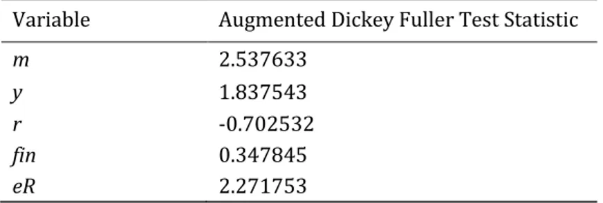
The first empirical analysis involved testing the time series properties of the data. Using the formulation given earlier, the study tests the hypothesis of a unit root in level variables. The results are given in Table 1 below:
Table 1. Unit root results for level variables
Variable Augmented Dickey Fuller Test Statistic
m 2.537633
y 1.837543
r -0.702532
fin 0.347845
eR 2.271753
The critical value for the tests at 5% is -2.9527
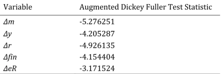
Table 2. Unit root results for first difference variables
Variable Augmented Dickey Fuller Test Statistic
Δm -5.276251
Δy -4.205287
Δr -4.926135
Δfin -4.154404
ΔeR -3.171524
The critical value for the test at 5% is -2.9558
The ADF test statistics for all the variables in the table above have exhibited the expected excess negativity relative to the critical value of -2.9558. Thus all of them achieve stationarity after first difference. The variables are therefore integrated of order one (I(1)).
4.2.
Co-integration test
2Owing to the fact that all the variables in the model are integrated of order one, i.e ~ I(1), the researcher sought to establish whether the variables were in any way related, in the long-run. When variables have along run equilibrium relationship, they are said to be cointegrated. To undertake the cointegration test the Johansen Cointegration Procedure was employed. The results of this procedure are presented below:
Table 3. Johansen cointegration procedure (Series: myrfineR)
Eigen Value Likelihood Ratio 5% Critical Value 1% Critical Value Hypothesised N0. Of CE(s)
0.738984 111.6764 94.15 103.18 None**
0.558956 68.69477 68.52 76.07 At most 1*
0.419999 42.49921 47.21 54.46 At most 2
0.318063 25.06801 29.68 35.65 At most 3
0.312097 12.81784 15.41 20.04 At most 4
0.026103 0.846405 3.76 6.65 At most 5
*(**) denotes rejection of the hypothesis at 5%(1%)
L.R test indicates 2 cointegrating equations at 5% significance level
The results of the Johansen procedure indicate 2 cointegrationg vectors thereby confirming cointegration i.e the variables have a long run equilibrium to which they converge. Apart from justifying a short-run error correction model, these results also confirm the stability of the money demand function. Thus, by these results, Keynes’s contention of a relatively unstable demand function is challenged.3
2 We also confirmed cointegration using the Engle-Granger Two Step Procedure. By this procedure the errors were stationary in
levels (ADF Stat = - 4.2457).
4.3.
The error correction model
With cointegration confirmed the next step is to run an Error Correction Model of the following form:
m
m
teR
fin
r
y
m
0 1 2 3 4 5 1
(10)
where
is the difference operator,
1 ˆ m m
is the Error Correction Mechanism. We have the results in the table 4.
4.4.
Interpretation of the results and policy implications
The first to note regarding the regression results is the adjusted R-squared. This statistic shows the percentage variation in the dependent variable explained by the explanatory variables. It is an unbiased measure. The adjusted R-squared of 0.785 indicates that about 79% of the variation in real money demand has been explained by the independent variables. This is a good fit. The good fit, is reinforced by Ramsey RESET test which confirms that the model is well specified.
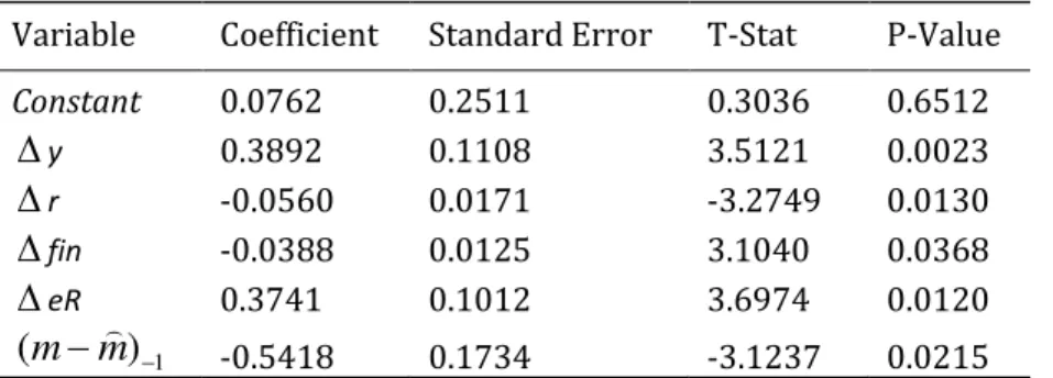
Table 4. Estimated short-run error correction results
(Dependent variable: m: Log of real money balances)
Variable Coefficient Standard Error T-Stat P-Value
Constant 0.0762 0.2511 0.3036 0.6512
y 0.3892 0.1108 3.5121 0.0023
r -0.0560 0.0171 -3.2749 0.0130
fin -0.0388 0.0125 3.1040 0.0368
eR 0.3741 0.1012 3.6974 0.01201
)
(
m
m
-0.5418 0.1734 -3.1237 0.0215R0.785; RESET Test (F-Stat: 0.402280, P-Value: 0.673046);
BG-Serial LM Test (F-Stat: 0.046083, P-Value: 0.955043); White Test (Obs*R-
Squared: 6.625259, P-Value: 0.760286), VIF (2.14)
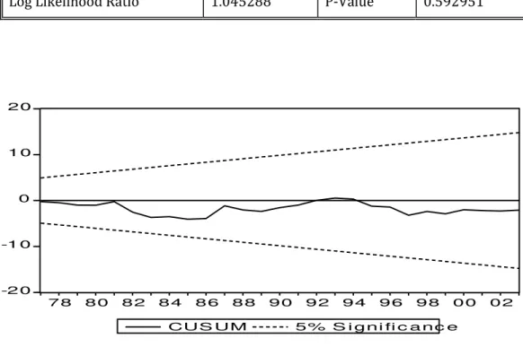
The regression results in table 4 can only be meaningful if the modelling process is devoid of the common econometric problems. In terms of assessing the stability of the short-run demand function it has been shown that the money demand function for Malawi is stable by the Cusum Test, and the Recurcive Test.4 These tests
show that money demand function is stable, again reinforcing the earlier result, on cointegration. Thus once again, it can be emphasised that the Keynesian contention of a relatively unstable money demand function, does not hold in Malawi. Further, the Breusch Gofrey Serial LM Test has a high p-value indicating that the model’s disturbances are not serially correlated. Similarly the White (eteroscedasticity Test exhibits a high
p-value, refuting the hypothesis of non-homogeneity of variance.5 Furthermore, the explanatory variables
were also not victims of multicollinearity as the Variance Inflation Factor (VIF) is clearly less than 5, from table 4 above.
After achieving an econometrically sound model the coefficients of the regression line can now be examined. First, the income elasticity of demand for money bears the expected positive sign as argued by Keynes. It is also significant at the 1% level. Empirically the positive sign is in line with many other studies on money demand (See for example, Jose R. Sanchez-Fung, and Cigdem Izgi Kogar, 1995). The positive sign confirms the Keynesian assertion that real income is positively linked to demand for transactions and precautionary money balances. The results also show that an increase in real income increases money demand inelastically in Malawi. This crucially contradicts results of studies in the developed countries such as that of Meltzer (1999) which established an income elasticity of greater than unity. Implicitly, one can argue that the results are not unexpected in the case of Malawi where real incomes are generally low, perhaps emphasising that, demand is income driven. Realistically this result lays in the open the fact that policies consistent with raising real incomes in Malawi are urgent.
The interest elasticity is negative as expected and statistically significant. While this is in concomitant with the predictions of the Keynesian speculative argument, it crucially contradicts the Keynesian expectation of an elastic interest rate. Thus for the case of Malawi the empirically determined interest elasticity deeply betrays Keynes theoretical forecasts.
The variable for financial sector development exhibits a negative significant coefficient. These results are in line with those of Shawa (2004) who estimated an income velocity of money equation and found a positive sign linking financial sector development and velocity ( a negative sign is implicit for the money demand equation)6. The negative sign implies that when the financial sector develops people have a wide choice to
balance their portifolio. For example with the existence of stock exchange markets people can buy stocks and shares. This sheds a picture that the Malawian Financial Sector is fairly well developed. However the fact that the coefficient is insignificant points to the fact that the financial sector is yet to fully develop for optimal results. This implies that deliberate policies to improve the financial sector should be encouraged in Malawi.
The exchange rate measures the financial risk of substituting the domestic currency for a foreign one. The results show a positive significant parameter for exchange rate. It implies that as the Kwacha increases (as it depreciates) people would rather hold the money than allow it to be eroded in the financial system. In such cases people demand the domestic currency so that they can buy foreign currency such as the dollar to hedge themselves against exchange losses. This calls for urgent exchange rate management policies in Malawi.
The one-period lagged error term is negative and statistically significant at1% level. Its coefficient which is approximately-0.54 implies that about 54% of the discrepancy between actual and equilibrium value of money demand is corrected each period. Thus there are economic forces in the economy which operate to restore the long-run equilibrium path of the money demand following short-run disturbances.
5 See Appendix Two for the details of the tests
6 See Shawa K. C (2004), Determinants of the Velocity of Circulation in Malawi: An Error Correction Approach, Eastern Africa Journal
4.5.
Was Keynes right? implications of his propositions
To discuss the implications of the findings of the study in relation to Keynes’s propositions a quotation from Sloman (1997, pp 573) is in order:
…Keynesians argue that the money demand curve is relatively elastic and unstable…, Monetarists argue that
it is relatively inelastic and stable
From the quotation above and what has already been argued in the paper, Keynes proposed an unstable demand function with an elastic interest elasticity of money demand. The results of this study, however, have shown that the demand for money function in Malawi, is stable. This has been accomplished by the both the cointegration test and the stability tests. Thus one can argue that the present results point to the direction of the Monetarist argument of a stable function. Thus the Keynesian proposition of the unstable money demand function cannot be confirmed in Malawi.
There is no contention between monetarists and Keynesians on the positive link between real income and demand for money. In line with the arguments of both of them, the income elasticity of money demand in Malawi is positive.
(owever although the negative sign is also confirmed for the interest elasticity, Keynes’s argument that the interest rate elasticity of money demand is elastic, is contradicted in our study. The study actually establishes a very inelastic interest rate elasticity of money demand (-0.05) which, again, one can argue, is in line with the arguments of monetarists.
These findings imply that monetary policy in Malawi should be conducted with consideration that the money demand function is stable and that the interest elasticity of money demand in Malawi is inelastic.
5.
Conclusion and direction for further research
The main objective of the paper was to assess the validity of the Keynesian propositions on Money Demand and assess their implication on the conduct of monetary policy in Malawi. The paper used modern time series methods to clear the data of any statistical problems before estimating an error corrected model.
In line with Keynes proposition the study establishes a positive income elasticity of money demand and a negative interest elasticity of money demand. (owever contrary to Keynes’ postulates the study establishes a stable money demand equation for Malawi and inelastic interest elasticity. Monetary policy in Malawi therefore should be undertaken bearing in mind the stability of the money demand function and the less than proportionate response of money demand to interest rate changes.
In achieving the results the present work used annual time series data from 1970 to 2005. One can argue that more information can be obtained if quarterly data were used (not always the case). Further, this study has used time series data for one developing country. One may argue that a panel data analysis of all the
study. Nevertheless, the current study has laid an important foundation to the debate and the challenges mentioned herein remain the direction of future research for the author and other interested researchers.
Refernces
Andersen, P. , The stability of money demand functions: An alternative approach , working paper no. 14, Bank of International Settlements, Basle, April.
Arrau, P., De Gregorio, J., Reinhart, C. and Wickham, P. , The demand for money in developing countries: Assessing the role of financial innovation , working paper no. , The World Bank, New York, July.
Ball, L. , Short-run money demand , working paper no. , National Bureau of Economic Research, Cambridge, United Kingdom.
Ball, L. , Another look at long-run money demand , working paper no , National Bureau of Economic Research, Cambridge, United Kingdom.
Barnett, W. A., Fisher, D. and Serletis, A. , Consumer theory and the demand for money , Journal of Economic Literature, Vol. 30, No. 4, pp. 2086-2119.
Baumol, W. J. , The transactions demand for cash: An inventory theoretic approach , Quarterly Journal of Economics, Vol.66, pp. 545-546.
Granger, C.W.J. and Newbold, P. , Spurious regression in econometrics , Journal of Econometrics, Vol. 2, pp. 111-120.
Greiber C. and W. Lemke , Money demand and macroeconomic uncertainty , working paper no. , Deutsche Bundesbank, Frankfurt.
Hudson, J. (1982), Inflation: A Theoretical Survey and Synthesis, George Allen and Unwin, London.
IMF (2006), International Financial Statistics, (IFS), Washington D.C
Jackson, T. M. (1986), Basic Concepts in Monetary Economics, Checkmate Publications, United Kingdom.
Alan, C. and Sánchez-Fung. J. R. , Modelling money demand in the Dominican Republic , Application Economics, Vol. 32, No. 11, pp. 1439-1449.
Kogar, C. ). , Cointegrationtest for money demand: The case for Turkey and )srael , working paper no. 9514, The Central Bank of the Republic of Turkey, May.
Laidler, D. (1977), The Demand for Money: Theories and Evidence, Harper and Row Publishers, New York.
Laidler, D. (1990), The Foundations of Monetary Economics, Edward Edgar Publishing Limited, United Kingdom.
Laidler, D. , Notes on the microfoundations of monetary economics , Economic Journal, Vol. 107, No. 443, pp. 1213-1223.
Meltzer, A.(. , The demand for money: The evidence from time series , Journal of Political Economy,
Vol. 71, pp. 219-246.
Meltzer, A. (. , Limits of short-run stabilisation policy, Economic Inquiry, Vol. 25, No. 1, pp. 1-14.
Meltzer, A. (. , Commentary: monetary policy at zero inflation , in new challenges for monetary policy: A symposium sponsored by the Federal Reserve Bank of Kansas City, pp. 261-276.
Qayyum, A. , Modelling the demand for money in Pakistan , The Pakistan Development Review, Vol. 44, No. 3, pp. 233-252.
Sato, L. , Monetary frameworks in Africa: The case of Malawi , paper presented at an international conference on monetary policy frameworks in Africa, 17 September-19 September, Pretoria, South Africa, available at http://www.resbank.co.za/Lists/ News%20Publications/Attachments/57/Malawi:pdf(accessed, 20 March, 2010).
Shawa, K.C. , Determinants of the Velocity of Circulation in Malawi: An Error Correction Approach,
Eastern Africa Journal of Humanities and Sciences, Vol.4, No.2, pp. 56-70.
Sloman, J. (1997), Economics, Prentice Hall, London.
Treichel, V. , Broad money demand and monetary policy in Tunisia , working paper no. / , International Monetary Fund, Washington.
Tobin, J. , The interest elasticity of the transactions demand for cash , Review of Economics and Statistics, Vol. 38, No. 3, pp. 241-247.
Appendix 1. Stability tests
The Ramsey RESET test
This is a regression error specification test (RESET) which was proposed by Ramsey in 1969. It tests specification errors of omitted variables, incorrect functional form and correlation between the independent variables and errors. It is therefore a general test of stability. In our model the null hypothesis of stability cannot be rejected since (as can be seen from the table below) the P-values for both the F-Stat and the Log-Likelihood Ratio confirm the insignificance of the statistics.
The Cusum test
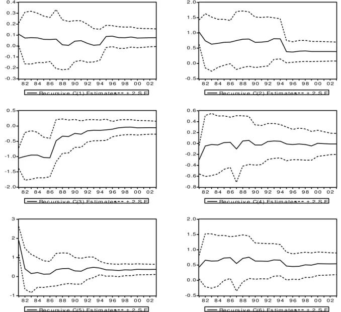
The recursive coefficient test
This test allows a trace of the evolution of estimates for every coefficient. If the coefficient displays significant variation to the estimating equation, it is a strong indication of instability. Coefficient plots may also show dramatic jump as the postulated equation tries to digest a structural break.
Table 5. Results of the Ramsey RESET test
F-Statistics 0.402280 P-Value 0.673046
Log Likelihood Ratio 1.045288 P-Value 0.592951
Figure 1. Results of the CUSUM stability test
It is important to note that C(1) represents the evolution of the constant term, C(2) represents the evolution of the coefficient of real GDP, C(3) represents the evolution of the coefficient of interest rate, C(4) represents the evolution the coefficient of financial development, C(5) represents the evolution of the coefficient of exchange rate and the evolution of the coefficient of the on period lagged error correction term is represented by C(6) .These recursive estimates show very stable evolution without any structural break and therefore the hypothesis of parameter stability is confirmed.
-2 0 -1 0 0 1 0 2 0
7 8 8 0 8 2 8 4 8 6 8 8 9 0 9 2 9 4 9 6 9 8 0 0 0 2
Figure 2. Results of the recursive coefficient test
Appendix 2. Residual tests
The results of stability obtained above and the regression results can be challenged should the residual tests fail to obtain. We thus undertake to demonstrate that the models use does not have autocorrelated errors, heteroscedastic errors, and abnormal errors. We use the Breusch-Godfrey serial correlation LM test to test for serially correlated errors. We use the White test to assess variance homogeneity.
-0 .3 -0 .2 -0 .1 0 .0 0 .1 0 .2 0 .3 0 .4
8 2 8 4 8 6 8 8 9 0 9 2 9 4 9 6 9 8 0 0 0 2
Re c u rs i v e C(1 ) Es ti m a te s ± 2 S.E.
-0 .5 0 .0 0 .5 1 .0 1 .5 2 .0
8 2 8 4 8 6 8 8 9 0 9 2 9 4 9 6 9 8 0 0 0 2
Re c u rs i v e C(2 ) Es ti m a te s ± 2 S.E.
-2 .0 -1 .5 -1 .0 -0 .5 0 .0 0 .5
8 2 8 4 8 6 8 8 9 0 9 2 9 4 9 6 9 8 0 0 0 2
Re c u rs i v e C(3 ) Es ti m a te s ± 2 S.E.
-0 .8 -0 .6 -0 .4 -0 .2 0 .0 0 .2 0 .4 0 .6
8 2 8 4 8 6 8 8 9 0 9 2 9 4 9 6 9 8 0 0 0 2
Re c u rs i v e C(4 ) Es ti m a te s ± 2 S.E.
-1 0 1 2 3
8 2 8 4 8 6 8 8 9 0 9 2 9 4 9 6 9 8 0 0 0 2
Re c u rs i v e C(5 ) Es ti m a te s ± 2 S.E.
-0 .5 0 .0 0 .5 1 .0 1 .5 2 .0
8 2 8 4 8 6 8 8 9 0 9 2 9 4 9 6 9 8 0 0 0 2
The Breusch-Godfrey serial correlation LM test
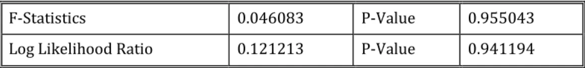
Developed by Gofrey (1988) this is a Lagrange Multiplier test which test for higher order serial correlation. The null hypothesis for the test is that there is no serial correlation of up to order (P) where p is specified by the researcher. In the present case we choose the commonly used order 2. Both the F-Stat and Loglikelihood Ratio cannot be rejected at any conventional significant levels as can be seen in then table below
Table 6. Results of the Breusch-Godfrey serial LM test
F-Statistics 0.046083 P-Value 0.955043
Log Likelihood Ratio 0.121213 P-Value 0.941194
The White heteroscedasticity test
The test was developed by White (1980). It tests the presence of dynamic error variance under the null hypothesis of homoscedasticity. Again the results below clearly confirm homoscedasticity.
Table 7. Results of the White heteroscedasticity test
F-Statistics 0.552634 P-Value 0.833786