* Corresponding author: E-mail: [email protected]
Received: February 6, 2018 Approved: June 26, 2018
How to cite: Horst TZ, Dalmolin RSD, ten Caten A, Moura-Bueno JM, Cancian LC, Pedron FA, Schenato RB. Edaphic and topographic factors and their relationship with dendrometric variation of Pinus Taeda L. in a high altitude subtropical climate. Rev Bras Cienc Solo. 2018;42:e0180023.
https://doi.org/10.1590/18069657rbcs20180023
Copyright: This is an open-access article distributed under the terms of the Creative Commons Attribution License, which permits unrestricted use, distribution, and reproduction in any medium, provided that the original author and source are credited.
Division - Soil in Space and Time | Commission – Soil Genesis and Morphology
Edaphic and Topographic Factors and
their Relationship with Dendrometric
Variation of
Pinus Taeda
L. in a High
Altitude Subtropical Climate
Taciara Zborowski Horst(1)*
, Ricardo Simão Diniz Dalmolin(2)
, Alexandre ten Caten(3)
, Jean Michel Moura-Bueno(1)
, Luciano Campos Cancian(1)
, Fabrício de Araújo Pedron(2)
and Ricardo Bergamo Schenato(2)
(1)
Universidade Federal de Santa Maria, Departamento de Solos, Programa de Pós-Graduação em Ciência do Solo, Santa Maria, Rio Grande do Sul, Brasil.
(2)
Universidade Federal de Santa Maria, Departamento de Solos, Santa Maria, Rio Grande do Sul, Brasil. (3)
Universidade Federal de Santa Catarina, Departamento de Agricultura, Biodiversidade e Florestas, Curitibanos, Santa Catarina, Brasil.
ABSTRACT: The study of the relationships between the yield potential of forest stands
and the conditions offered for plant development is fundamental for the adequate
management of the forest when aiming at sustainable high yields. However, these relations are not clear, especially in commercial forests, on rugged terrain where relationships between the landscape, soil, and plants are more complex. Considering this, we tested the hypothesis that the morphological aspects of the soil conditioned by topography are the main limiting factors for tree development. Our objective was to
evaluate the edaphic and topographic influence on the dendrometric variation of Pinus taeda L. of a forest stand in a subtropical climate at high altitude. For that, Spearman’s correlation analysis and canonical correspondence were performed on two data datasets containing pedological, topographic, and dendrometric information of a commercial
plantation of Pinus taeda, in the Campo Belo do Sul, Santa Catarina state, Brazil. Soil
sampling and characterization was performed in two distinct designs. The first design was based on the morphological description of 11 soil profiles. The second was performed
with intensive prospecting of the area, with 102 sampling locations determined through conditioned Latin hypercube sampling. For each sampling point, the height and diameter of the four nearest trees were measured and the terrain attributes were calculated from
the digital elevation model. The solum depth, the thickness of the superficial horizon,
elevation, and vertical distance to channel network were the main conditioning factors of the dendrometric variation, wherein taller trees were found in deeper soils, with a thicker surface horizon, in lower areas that are vertically closer to the drainage network. Our results showed that the selection of topographic and morphological variables has a
significant effect on the tree height and should therefore be used to select homogeneous
areas for the development of the species. In addition, we showed the importance of using an intensive sampling survey to understand dendrometric variation.
INTRODUCTION
Understanding the edaphic and topographic influence on forest development is essential
for rational management of forest and soil. Studies relating forest development to soil conditions are common for native forests (Zhang et al., 2016; Mendonça et al., 2017; Oberhuber, 2017; Soboleski et al., 2017 ), showing the strict relationship between soil, relief, and forest, and highlighting the importance of studying these relationships at the landscape scale. However, in commercial forests, these relations are not clear, especially in rugged terrain where relationships between the landscape, soil, and plants are more complex.
According to the annual report of the Brazilian Tree Industry (Ibá, 2017), Brazil led the global
ranking of pine forest yield in 2016, with an average 30.5 m³ ha-1
yr-1
in pine plantations, with plantations predominantly concentrated in the south of the country. To improve the
efficiency of forest production and supply the current and future demand for feedstock,
the forestry sector seeks to incorporate information about soil and relief to plan planting
and operations. Using such information, it is possible to increase profitability and adjust
production to the support capacity of the soil, establishing management units and zoning for silviculture and directing the use of capital and technology in areas of interest
(Costa et al., 2009; Gomes et al., 2016). That demands an elucidation of questions related
to the yield potential and main limiting factors for production in certain areas. There are
several studies relating Pinus taeda to soil properties, such as particle size distribution
(Rigatto et al., 2005; Dedecek et al., 2008), organic matter (Gonçalves et al., 2012), solum depth (Morales et al., 2010), and pH (Barbosa et al., 2012). Nonetheless, these evaluations seldom consider relief information and restrict sampling to groups of plots from a continuous inventory, disregarding the variability of soil and topography along the landscape. In addition, these studies normally consider only physical and chemical variables as edaphic factors. However, morphological properties such as solum depth
and the thickness of the A horizon can limit the expression of the effect of chemical and
physical variables on the forest (Castelo et al., 2008), especially in regions of complex relief where pine forests are most common in Brazil (Gomes et al., 2016; Ibá, 2017).
Since tree growth is affected by the environment, a detailed study of these relationships
can be useful to establish methodologies to direct resources, besides providing a basis for zoning and for calibration and validation of ecophysiological models that will help forest management. Moreover, increasing the knowledge about forest dynamics may be useful to show possible adaptations of the forest facing climate change, as observed in McDowell and Allen (2015) and Brandt et al. (2017).
Considering the edaphic and topographic variability present along the landscape, we tested the hypothesis that morphological aspects of the soil conditioned by topography are the main limiting factors for tree development. Hence, our objective was to evaluate
the edaphic and topographic influence on the dendrometric variation of Pinus taeda L. specimens of a forest stand in a subtropical climate at high altitude.
MATERIALS AND METHODS
Characterization of the study area
The study was conducted in a stand of Pinus taeda L. on first rotation, aged 29 years,
in Campo Belo do Sul, the mountain region of Santa Catarina state, Brazil (Figure 1a). The area covers 108 ha (Figure 1b) and has no history of soil chemical correction. The predominant climate type is Cfb (Alvares et al., 2013), mesothermic, subtropical humid, and with an average well-distributed annual precipitation of 1,647 mm. The regional
Soil sampling and characterization was performed in two distinct designs: morphological
description and intensive prospecting. The first design was based on the morphological description of 11 soil profiles (Figure 1b), representing the study area, according to the
methodology described in Santos et al. (2015). The locations of the descriptions were
intentionally distributed from the valley to the top of the toposequence.
Disturbed soil samples were collected in each horizon of the described profile for chemical characterization and particle size distribution, as well as five undisturbed samples to
determine soil density (Ds), microporosity (Mi), macroporosity (Ma), total porosity (TP), and saturated hydraulic conductivity (Ks). The analyses were performed according to Donagema et al. (2011). The data were called dataset number 1.
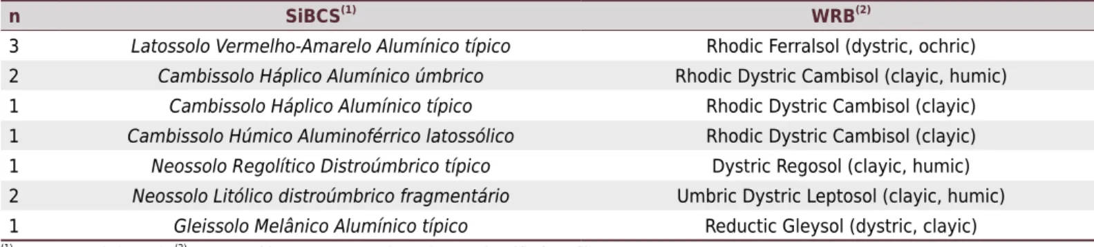
Soils were classified both in Sistema Brasileiro de Classificação de Solos (SiBCS) (Santos et al., 2013) and the World Reference Base for Soil Resources of the FAO (IUSS Working Group WRB, 2015), according to table 1. Our results will be discussed according to SiBCS (Santos et al., 2013).
To represent the variability of the landscape according to the characteristics of the terrain, a second sampling design was performed with intensive prospecting of the area, establishing 102 sampling locations (Figure 1b). The sampling locations were determined through conditioned Latin Hypercube Sampling (cLHS) (Minasny and McBratney, 2006). At each location, soil samples were collected for particle size distribution from layers 0.00-0.20,
(b) 517000 517500 518000 518500
6909540
6909105
Legenda
Elevation (m) 865 879 893 907 920 935 0 100 200 300 400 m
Transect
Campo Belo do Sul N
Study area
Study area Data set 1 Data set 2
A A'
6908670
6900000
6920000
6940000
506000 528000
N (a)
Figure 1. Location of the study area in the Campo Belo do Sul, Santa Catarina state (SC), Brazil (a) and enlarged area with digital
elevation model and distribution of data datasets (b), where the transect indicates the typical toposequence.
Table 1. Correlation between the Brazilian Soil Classification System and Word Reference Base used for soil dataset 1
n SiBCS(1)
WRB(2)
3 Latossolo Vermelho-Amarelo Alumínico típico Rhodic Ferralsol (dystric, ochric) 2 Cambissolo Háplico Alumínico úmbrico Rhodic Dystric Cambisol (clayic, humic) 1 Cambissolo Háplico Alumínico típico Rhodic Dystric Cambisol (clayic) 1 Cambissolo Húmico Aluminoférrico latossólico Rhodic Dystric Cambisol (clayic) 1 Neossolo Regolítico Distroúmbrico típico Dystric Regosol (clayic, humic) 2 Neossolo Litólico distroúmbrico fragmentário Umbric Dystric Leptosol (clayic, humic) 1 Gleissolo Melânico Alumínico típico Reductic Gleysol (dystric, clayic)
(1)
0.20-0.40, 0.40-0.60, and 0.60-1.00 m. Particle size distribution was represented by the average of the layers. Besides, morphological variables, solum depth (SoD) up to 1.00 m, and the thickness of the A horizon (TAH) were measured according to Lepsch et al. (2015).
The dendrometric variables measured were diameter at breast height (DBH) using a tape measure and total tree height (h) using a vertex. The sample intensity of trees was
defined to represent a resolution pixel of 10 meters (100 m²), wherein the four P. taeda
individuals closest to each sampling location were measured. The average height and DBH of the four trees were used to represent each sampling location for datasets 1 and 2.
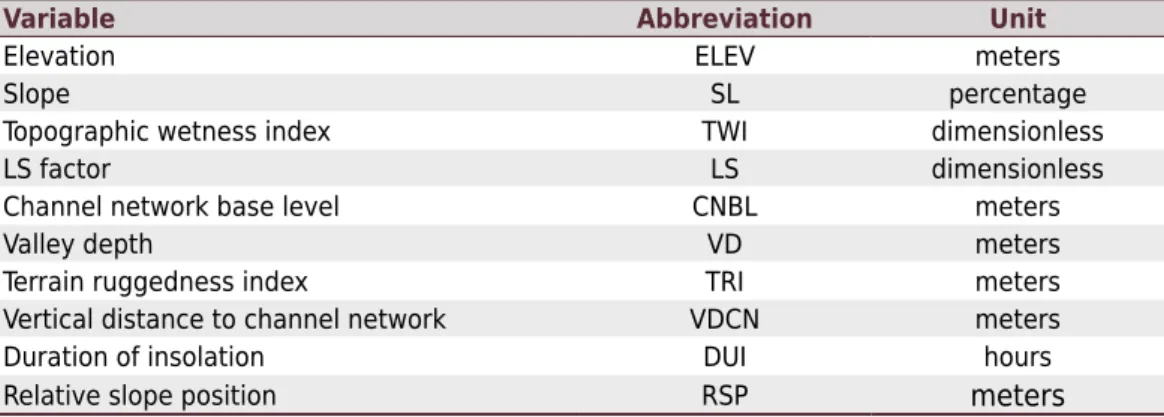
Twelve topographic variables (Table 2) were derived from a digital elevation model (DEM) (Sigsc, 2010) with a resolution of 10 m, according to Wilson and Gallant (2000). Processing was performed in SAGA GIS (Conrad et al., 2015).
Descriptive statistics were obtained for soil, dendrometric, and topographic variables in datasets 1 and 2. For physical and chemical variables of dataset 1, the average of the horizons
A and B of each profile was calculated, to later calculate the average of the soil class, thus avoiding the influence of the number of horizons in the mean. The hypothesis of normality
and homoscedasticity of the data was tested through the Shapiro-Wilk test (5 % probability).
The relationship between variables was evaluated through matrices of linear data correlation for each data dataset through Spearman’s method, in which edaphic and topographic variables were correlated with dendrometric variables. Canonical correspondence analysis (CCA) was
used to test if the edaphic conditions significantly explain the dendrometric variations. Two
matrices were prepared as follows: a vegetation matrix with dendrometric variables DBH
and h, the latter classified in four height levels (in decreasing order: h1, h2, h3, and h4),
and an environmental matrix with edaphic and topographic data. The Monte Carlo test was
used with 999 permutations in order to test the significance of the correlations. All statistical
analyses were performed in the R environment (R Development Core Team, 2017).
RESULTS AND DISCUSSION
Characterization and correlation of variables in dataset 1
Deep soils were identified at well-drained locations with flat or gentle slope relief, with a sequence of horizons A-Bw (Latossolo Vermelho-Amarelo Alumínico típico), while soils with a
sequence of horizons A-Cg occurred in poorly-drained conditions (Gleissolo Melânico Alumínico típico). In steep and strongly steep relief, we observed soils with a sequence of horizons A-Cr
or A-Bi (Neossolo Regolítico Distroúmbrico típico, Cambissolo Háplico Alumínico úmbrico,
CambissoloHáplico Alumínico típico, and Cambissolo Húmico Alumino férrico latossólico) and
soils with a sequence of horizons A-R and A-CR (Neossolo Litólico distroúmbrico fragmentário)
(Figure 2). The number of profiles described in each soil class is shown in table 2.
Table 2. Topographic variables derived from the digital elevation model (DEM) with their respective
abbreviations and units
Variable Abbreviation Unit
Elevation ELEV meters
Slope SL percentage
Topographic wetness index TWI dimensionless
LS factor LS dimensionless
Channel network base level CNBL meters
Valley depth VD meters
Terrain ruggedness index TRI meters
Vertical distance to channel network VDCN meters
Duration of insolation DUI hours
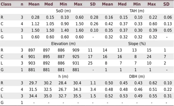
Neossolos are located at altitudes that vary from 886 to 909 m, with slopes greater
than 13 % (Table 2). In these conditions, the topographic gradient can reduce infiltration rates and increase runoff, accelerating erosion processes and the removal of superficial
horizons of the soil. Adding resistance of the parent material and slope instability, soils observed in these areas were shallow, with an average SoD of 0.28 m, median of 0.15 m,
and superficial horizon around 50 % shallower than the other classes (Table 3).
Cambissolos were identified predominantly in convex slopes, distributed in gently
undulated relief (minimum slope = 8 %), as well as strongly undulated relief (maximum slope = 24 %), which were moderately deep (0.90 m) to deep (1.50 m). In relation to TAH,
the mean and median in Cambissolos were 0.42 and 0.33 m, respectively (Table 3). The
Latossolos were between 892 and 931 m and 8 % of the average slope, which enables
the pedogenetic development of the profile at greater depths, mainly expressed by SoD
above 1.40 m (Table 3).
Gleissolos occurred in flat valleys, which hinder the vertical and lateral movement of
water and sediments, creating poor drainage conditions. They are moderately deep
soil (0.60 m) with a superficial horizon of 0.32 m (Table 3), located primarily in areas of
permanent preservation. Since they are not located in productive areas, the information about this soil class was not considered for statistical analyses.
The development of P. taeda was different on Neossolos and Latossolos. While in the
Neossolos the average tree height reaches 29.7 m, in the latter it is up to 34.4 m (Table 3). The standard deviation (SD) is small (1.1 and 1.5 m, respectively) and the mean values
0 200 400 600
Distance (m)
Elevation (m
)
890
900
910
920 30 m
Soil depth 0.70 m
Cambissolo Háplico Rhodic Dystric Cambisol
Neossolo Litólico Dystric Regosol
Latossolo Vermelho-Amarelo
Rhodic Ferralsol Gleissolo Melânico Reductic Gleysol
Neossolo Regolítico Dystric Regosol 0.10 m
A
0.4 m
0.1 m
0.35 m
0.3 m
0.25 m Bi
A
R
A
Bw
A
Cg
A
Cr 1 m
0.25 m
27 m
35 m
28 m
800 1000
Figure 2. Relationship between soil class, soil depth and tree height of a Pinus taeda commercial plantation in a typical toposequence
are very close to the medians in both classes. In Cambissolos, trees with an average height of 31.5 m were found, with a high dispersion of data (SD = 3.4 m) (Table 3). The
variance in TAH on Cambissolos might be the cause of the dissimilarities in yield and
tree development in this soil class.
The specimens of P. taeda on Latossolos showed the highest DBH values, with an average
of 0.52 m, varying from 0.49 to 0.55 m (Table 3). However, those that developed on
Neossolos showed an average diameter greater than those on Cambissolos (0.50 and
0.48 m, respectively), a consequence of the extreme values in the mean of the first
class (maximum = 0.62 m), also observed in the high standard deviation (10.4). Similar results were found by Rachwal et al. (2008), evaluating the relationship between black
wattle (Acacia mearnsii) and edaphic variables, who found lower values for DBH and
height in areas of Neossolos when compared to the values found in areas with deeper
soils, such as Cambissolos.
Gomes et al. (2016), with the objective of developing and applying a methodology to
establish management units for Pinus by mapping soil classes in the west of Santa
Catarina, pointed out that the limitations associated with the effective depth of soil, relief,
and stoniness/rockiness made the impediments for management the most important limiting factors for cultivation of pine trees. Nevertheless, the ability to identify the most productive areas using only soil classes depends on whether the limiting factors for plant
development in the area are or are not differential characteristics or covariates in the system for soil classification used (Resende et al., 2012).
The same pattern related to height is identified in DBH medians (0.45 m in Neossolos,
0.48 m in Cambissolos, and 0.53 m in Latossolos). These results corroborate those of
Dedecek et al. (2008), who found a significant difference between DBH values studying
the same soil classes.
In relation to the chemical variables, the profiles showed pH(H2O) values between 4.6 and 4.8, with a tendency to increase with depth. The superficial horizons of both soil
classes showed higher organic matter (OM) contents, varying around 4.3, 4.6, and 4.2 %
Table 3. Descriptive statistics of dendrometric, topographic, and morphological variables of soil
dataset 1 separated by soil class
Class n Mean Med Min Max SD Mean Med Min Max SD
SoD (m) TAH (m)
R 3 0.28 0.15 0.10 0.60 0.28 0.16 0.15 0.10 0.22 0.06
C 4 1.12 1.05 0.90 1.50 0.26 0.42 0.37 0.33 0.60 0.13
L 3 1.50 1.50 1.40 1.60 0.10 0.35 0.37 0.30 0.39 0.05
G 1 0.60 0.60 0.60 0.60 - 0.32 0.32 0.32 0.32
-Elevation (m) Slope (%)
R 3 897 897 886 909 11 14 13 13 15 1
C 4 901 895 887 925 17 16 16 8 24 7
L 3 903 892 886 931 25 8 7 7 10 2
G 1 881 881 881 881 - 1 1 1 1
-h (m) DBH (m)
R 3 29.7 30.2 28.4 30.4 1.1 0.50 0.45 0.43 0.62 0.10
C 4 31.5 32.5 26.7 34.3 3.4 0.48 0.48 0.46 0.51 0.22
L 3 34.4 35.0 32.7 35.5 1.5 0.52 0.53 0.49 0.55 0.31
G 1 - - -
for Neossolos, Cambissolos, and Latossolos, respectively. Phosphorus contents (P) were
considered very low according to CQFS-RS/SC (2016), varying between 1.3 mg dm-3
in B
horizons of Latossolos to 3.9 mg dm-3
in Cambissolos A horizons. The sum of bases (SB) decreases considerably as the degree of development of soil increases, varying between
5.2 cmolc dm-3 in Neossolos and 0.7 cmolc dm-3 in B horizons of Latossolos (Table 4).
Cation exchange capacity (CEC) values are medium to high (CQFS-RS/SC, 2016), with
higher values on topsoil due to the contribution of OM. The CEC was highest in Neossolos
(18.3 cmolc dm
-3
) and lowest in B horizons of Latossolos (7.3 cmolc dm
-3
). However, we can observe that most of the CEC of these soils is occupied by potentially toxic cations such
as Al3+
, given the Al % values (Table 4).
In relation to the physical variables, none of the soil classes showed textural difference
between horizons, with clay contents increasing according to the degree of development of
the soils (Table 3). The soil structure formed in the superficial layers is strongly affected by
OM, predominantly granular and lumpy, characterized by the high porosity of the aggregates. Because of this, comparatively, the subsurface layers with lower OM contents, showed higher
average Ds, reaching 1.18 Mg m-3
in Cambissolos and 1.25 Mg m-3
in Latossolos (Table 4).
Total porosity values were higher in superficial horizons and Ds increases at greater depths, increasing the frequency of micropores in relation to macropores (Table 4). Still in superficial
horizons, the average TP varied from 0.59 to 0.66 m3
m-3 in the different soil classes. These values were higher than those found by Morales et al. (2010) and Bognola et al. (2010)
in forests of P. taeda aged six and 12 years, respectively. These authors used a reference
value of 0.10 m3
m-3
for macropores as a minimum threshold for good aeration. Applying
the same criterion and considering the difference between TP and Mi, we observe that aeration is adequate in all the soil classes described in the study area (Table 4).
Values of Ks were sensitive to differences in soil classes. The A horizon of Neossolos
shows an average Ks of 716.8 mm h-1
and a high standard deviation (Table 4). Considering
that Neossolos has a low SoD (Table 3), a high Ks favors water drainage from the
system and can decrease the water availability for plants on these soils. In the A
horizons of Cambissolos and Latossolos, Ks is lower, showing values of 276.9 and
299.1 mm h-1
, respectively, and decreases considerably in B horizons, reaching an
average of 168.4 mm h-1
in Latossolos (Table 4).
The most significant results for correlation between variables in dataset 1 were observed with SoD and slope (Table 5). Tree height showed a significant positive linear correlation
with SoD (r = 0.71) and negative with slope (r = -0.89). The relationship of tree height with SoD and slope is explained by the strong importance of slope for pedogenetic
processes (Gallant and Wilson, 2000; Valeriano, 2008), which affects the soil’s water holding capacity, the potential for erosion/deposition, and consequently, the degree of
development of the soil, shown by the inverse relationship between terrain slope and SoD (r = -0.74).
Greater slopes in the landscape conditioned the formation of shallower soils in the study area, with higher amounts of primary materials and lower clay contents, which explains the correlation of slope with the variables Ks (r = 0.36), sand (r = 0.49), CEC (r = 0.40), and pH (r = -0.37) (Table 5). The correlation of the variables Ks and sand with height were negative (r = -0.52 and -0.54, respectively) (Table 5).
Tree height showed a linear correlation with Ds (r = 0.31), TP (r = -0.30), and Mi (r = 0.30). Soils with higher sand content, in landscape positions that favor leaching and low water
holding capacity, were also associated with the poorer growth rates of P. taeda by
Santos Filho and Rocha (1987). The results of Bognola et al. (2010) suggested that soils
present study can be attributed to the impositions indirectly caused by low SoD, since Ks and sand content are higher in shallower soils (Tables 3 and 4).
Less acidic soils resulted in taller trees, according to the linear correlation between pH and tree height (r = 0.41), although the correlations with the chemical variables
of the soil have not been expressive. Similarly, Rigatto et al. (2005) found significant correlations between yield and pH (r = 0.73), studying the influence of this variable on
the wood yield of P. taeda in Telêmaco Borba, PR. Furthermore, Barbosa et al. (2012)
presented the pH from the 0.00-0.20 m layer (r = 0.49) as an alternative to estimate
the wood yield of P. caribaea var. hondurensis in Brazilian Cerrado conditions. However,
according to CQFS-RS/SC (2016), forest species are tolerant of exchangeable Al in the
Table 4. Descriptive statistics of chemical and physical variables of soil dataset 1
Class Hor Mean Med Min Max SD Mean Med Min Max SD
pH(H2O) Assimilable P (mg dm
-3 )
R A 4.8 4.8 4.7 4.8 0.1 4.1 3.8 3.7 4.7 0.6
C A 4.7 4.7 4.5 4.9 0.2 2.5 2.4 1.7 3.5 0.7
B 4.8 4.8 4.7 4.9 0.1 1.3 1.3 0.6 1.9 0.6
L A 4.6 4.7 4.5 4.7 0.1 3.1 3.0 2.9 3.4 0.3
B 4.8 4.8 4.7 4.8 0.1 1.3 1.3 0.8 1.9 0.6
OM (%) SB (cmolc dm
-3 )
R A 4.3 3.8 3.8 5.2 0.8 5.2 5.9 3.2 6.5 1.8
C A 4.6 3.7 3.0 7.8 2.2 2.5 2.2 0.7 4.8 2.0
B 1.9 1.9 1.8 2.0 0.1 1.2 1.6 0.3 2.4 0.9
L A 4.2 4.3 3.9 4.5 0.3 3.1 2.8 2.2 4.3 1.1
B 1.3 1.3 1.3 1.4 0.1 0.7 0.7 0.6 0.9 0.2
CECpH7 (cmolc dm -3
) Al (%)
R A 18.3 17.8 17.6 19.4 1.0 53 48 43 67 13
C A 15.7 15.2 12.2 20.1 3.3 68 67 49 91 21
B 10.2 10.1 9.8 10.8 0.5 82 82 70 95 10
L A 13.9 14.6 10.9 16.1 2.7 70 67 65 78 7
B 7.3 6.6 5.9 9.4 1.9 86 86 81 90 5
Sand (g kg-1
) Clay (g kg-1
)
R A 127 120 114 148 18 560 565 540 573 18
C A 94 92 81 112 13 632 637 585 668 43
B 85 88 63 101 18 624 689 546 715 80
L A 75 75 57 94 18 622 636 585 646 33
B 55 60 44 62 10 688 682 680 700 11
Ds (Mg m-3) Ks (mm h-1)
R A 0.79 0.76 0.74 0.88 0.08 716 548 330 1272 493
C A 0.88 0.90 0.70 1.00 0.15 276 258 50 541 201
B 1.18 1.08 1.10 1.34 0.12 250 196 53 409 178
L A 0.93 0.90 0.90 1.00 0.06 299 311 257 328 37
B 1.25 1.01 1.00 1.31 0.12 168 207 46 251 107
TP (m³ m-³) Mi (m³ m-³)*
R A 0.66 0.67 0.62 0.69 0.04 0.46 0.47 0.41 0.50 0.05
C A 0.65 0.65 0.60 0.70 0.06 0.50 0.50 0.40 0.60 0.08
B 0.59 0.59 0.57 0.63 0.03 0.46 0.45 0.43 0.53 0.04
L A 0.63 0.60 0.60 0.70 0.06 0.50 0.50 0.50 0.50 0.01
B 0.59 0.60 0.58 0.60 0.01 0.47 0.50 0.40 0.50 0.06
soil and the response to liming is mainly attributed to the supply of Ca and Mg instead
of the correction of soil acidity, which does not mean that low pH does not affect the development of plants in specific cases.
In relation to SB, we did not find a significant linear correlation with height (r = -0.12), contrary to the findings of Rigatto et al. (2005), Bellote and Dedecek (2006), and Ruiz et al.
(2016). Likewise, OM showed r = -0.15 with height and r = -0.04 with DBH (Table 5). The possible explanation for the low negative linear correlation of SB and OM in this study is that the physical conditions have limited the development of the forest, long before fertility conditions. Similar conclusions were found by Castelo et al. (2008), in which
they point out the soil’s effective depth as a constraint in the worst sites, although they
highlight soil chemical properties as conditioning factors for better yields. Besides, as
discussed before, the tallest trees were found on Latossolos (Table 3), which have good
physical conditions and low nutrient contents (Table 4).
Since soil physical limitations had a more effective control on the growth response of the species than chemical ones, in the conditions of data dataset 1, we can affirm that
morphological soil variables prevailed over chemical ones in determining higher h and DBH.
Characterization and correlation of variables in dataset 2
The intervals of maximum and minimum SoD values were close to those found in dataset 1, with a minimum of 0.10 m, maximum of 1.50 m, mean of 0.59 m, median of 0.60 m, and standard deviation of 0.36 m. The thickness of the A horizon surpassed the maximum value previously found, rising from 0.60 m in dataset 1 to 0.70 m in dataset 2 (Figure 3). Furthermore, the average slope in dataset 2 increased considerably in relation to dataset 1,
comprising steeper areas (40 % maximum slope). This is a consequence of the larger
sampling area, collecting information from lower (879 m) and higher (934 m) elevations in relation to dataset 1. Because of the higher variance in data, the high correlations found in dataset 1 were diluted in dataset 2.
In dataset 2, SoD kept positive linear correlations with tree height and DBH, showing r = 0.39 and 0.26, respectively. Likewise, TAH showed r = 0.27 for height and r = 0.15
Table 5. Significant Spearman’s correlation coefficients between dendrometric, topographic, and
pedological variables of soil dataset 1
DBH h SLOPE ELEV
SoD *
0.48 *
0.74 *
-0.74 *
-0.36
TAH 0.05 0.24 -0.10 *
-0.35
SB -0.21 -0.18 0.16 -0.26
H+Al 0.23 -0.12 -0.01 0.17
CEC -0.12 *
-0.27 *
0.40 -0.17
Al % 0.24 0.15 -0.14 *
0.34
P -0.20 -0.07 0.09 0.01
OM -0.04 -0.15 0.10 -0.06
pH -0.06 *
0.41 *
-0.37 0.00
Ds -0.14 0.31 -0.09 0.12
TP 0.15 -0.30 0.10 -0.11
Ma 0.06 *
-0.42 -0.31 -0.23
Ks -0.04 *
-0.52 *
0.36 0.11
Sand -0.40 -0.54 0.49 -0.34
Clay 0.00 0.20 -0.04 0.21
DBH 1.00 0.29 *
-0.56 -0.08
h 1.00 *
-0.89 0.24
Clay (g kg-1)
Fr
equency
Sand (g kg-1) SoD (m) TAH (m)
n = 102 mean = 568 g kg-1 sd = 83 g kg-1 s = -0.9
n = 102 mean = 120 g kg-1 sd = 48 g kg-1 s = 1.2
n = 102 mean = 0.59 m sd = 0.36 m s = -0.01
n = 102 mean = 0.31 m sd = 0.14 m s = 0.05
n = 102 mean = 906 m sd = 13 m s = 0.2
n = 102 mean = 18 m sd = 11 m s = -0.1
n = 102 mean = 16 m sd = 11m s = 0.4
n = 102 mean = 0.31 sd = 0.3 s = 0.4
n = 102 mean = 12.6 % sd = 5.6 % s = 0.7
n = 102 mean = 0.9 m sd = 0.51 m s = 1.3
n = 102 mean = 6.0 sd = 1.5 s = 1.7
n = 102 mean = 897 m sd = 9.4 m s = 1.2
n = 102 mean = 11.4 h sd = 0.4 h s = -0.6
n = 102 mean = 1.4 sd = 1.0 s = 1.7
n = 102 mean = 0.46 m sd = 0.13 m s = 0.08 m
n = 102 mean = 31 m sd = 3 m s = 0.5
(a) (b) (c) (d)
(e) (f) (g) (h)
(i) (j) (k) (l)
(m) (n) (o) (p)
0
300 500 700
51 02 03 0 05 10 15 05 10 15 20 05 10 15 20 25 05 10 15 20 25 01 02 03 04 0 50
0 100 200 300
01 02 03 04 0 01 02 03 04 0
0.20 0.40 0.60 0.80 1.0 0.10 0.30 0.50 0.70
ELEV (m) VD (m) VDCN (m) RSP
880 900 920 0 10 20 30 40 0 10 20 30 40 -0.2 0.2 0.6 1.0
05 10 15 01 02 03 04 05 0 01 02 03 04 0 01 02 03 04 0
SLOPE (%) TRI (m) TWI CNBL (m) 5 10 20 30 0.0 1.0 2.0 3.0 4 6 8 10 12 880 900 920
05 10 20 30 05 10 15 20 25 05 15 25 35 05 10 15
DUI (h) LS DBH (m) h (m)
10.0 11.0 12.0 0 1 2 3 4 5 6 0.40 0.45 0.50 0.55 24 28 32 36
for DBH (Figure 4). This result is similar to that obtained by Morales et al. (2010), who observed higher yields in sites with deeper soils. Corroborating this, Gomes et al. (2016),
when determining management units for pine trees, identified the variables effective
depth and relief as the main constraints for plantations in the west of Santa Catarina.
The particle size distribution did not show a significant influence on tree height, which is
in contrast with the results presented by Dedecek et al. (2008) and Rigatto et al. (2005), who found a relationship with soil texture. For both, heights were higher in clayey soils than in soils with medium texture. According to the authors, soils with higher sand contents and thus lower capacity to store water and nutrients showed lower yield potential. This is in line with a study by Oberhuber (2017), conducted in Australia, who showed that the water storage capacity of the soil is one of the factors that can limit radial growth in
pine trees. Besides not showing significant variation in soil texture along the landscape
(Figures 3a and 3b), rainfall is regular during the entire year in the study area (INPE, 2017). Thus, the importance of the particle size distribution in water retention that is pointed out by the cited authors might not be as important in subtropical areas at high
altitude where there is no significant textural gradient and/or variation.
The importance of slope to explain yield variations decreased from r = 0.74 in dataset 1 to r = 0.1 in dataset 2 in relation to height and from r = 0.48 to r = -0.06 in relation to
DBH (data not shown). On the other hand, elevation kept a correlation coefficient very
similar to the one obtained in dataset 1 (r = -0.45 in relation to height and r = -0.28 in
relation to DBH) (Figure 4). This result could be a reflection of the higher slope variation, which consequently smoothed these patterns among the heterogeneity of observations.
Therefore, when all the local variability is considered, the topographic variables elevation (ELEV) and vertical distance to channel network (VDCN) can be better indicators for yield.
This change in the behavior of the relationships and the reduction of the coefficients
(a)
r = -0.45 p < 0.001 40 35 30 25 880 900 ELEV (m) h (m) 920 (b)
r = -0.28 p < 0.004 0.60 0.55 0.50 0.40 0.45 880 900 ELEV (m) DBH (m) 0.60 0.55 0.50 0.40 0.45 DBH (m) 0.60 0.55 0.50 0.40 0.45 DBH (m) 0.60 0.55 0.50 0.40 0.45 DBH (m) 920 (c)
r = -0.44 p < 0.001 40
35
30
25
0 10 20 VDCN (m)
h (m)
30 0 10 20 30 (d)
r = -0.36 p < 0.001
VDCN (m) (e)
r = 0.39 p < 0.001 40 35 30 25 0.40 0.80 SoD (m) h (m)
1.20 0.40 0.80 1.20 0.20 0.40 0.60 0.20 0.40 0.60 (f)
r = 0.26 p < 0.008
SoD (m)
(g)
r = 0.27 p < 0.006 0.40 0.35 0.30 0.25 TAH (m) h (m) (h)
r = 0.15 p < 0.13
TAH (m)
Figure 4. Significant Spearman’s correlation coefficients between dendrometric, topographic, and pedological variables of dataset
of correlation between tree height and edaphic and topographic variables highlight the necessity to adopt viable strategies for a more intensive sampling along the landscape.
In relation to the topographic variables, VDCN and valley depth (VD) showed significant
correlation with tree height, r = -0.44 and 0.38, respectively. Regarding DBH, only VDCN proved relevant (r = -0.36). In order to understand these results, it is important
to consider that soils closer to the channel network are Neossolos, located on steep
slopes. As soon as the distance to the channel network increases, the slope decreases and more developed soils are found.
These results have been confirmed through CCA (Figure 5), which shows the canonical
correlations of edaphic variables in relation to dendrometric variables, represented by h, DBH, and h1, h2, h3, and h4. The two axes explained 71 % (axis 1) and 23 % (axis 2) of variance, with a total accumulated variance of 94 %. The Monte Carlo permutation test
showed that the dendrometric variables were significantly correlated with the edaphic
variables used, with p = 0.002.
The eigenvalues found for axes 1 and 2 were considered high (>0.5) according to ter Braak and Verdonschot (1995), for variables SoD (-0.61) and VD (-0.56) with the highest negative scores; and relative slope position (RSP) (0.58), ELEV (0.60), and VDCN (0.64) with the highest positive scores in CCA 1. Despite the low importance of CCA 2 (23 %), it shows a relevant negative score for channel network base level (CNBL) (-0.35) and positive for aspect (ASP) (0.38).
Hence, the two groups were clearly separated into a high-levels group (h1 and h2) and low-yield group (h3 and h4) (Figure 5). Axis 1, responsible for most of the variance, shows the highest negative scores for SoD and VD and positive scores for VDCN and
ELEV, suggesting the importance of these variables to differentiate environments for
the development of P. taeda.
CCA 2 (23 %)
CCA 1 (71 %)
-0.5 0.0 -0.5
0
-1.0 -0.5
0.0
-0.5
-0.5
TAH TRI
SoD
VD
SLOPE
LS
ASP
RSP VDCN ELEV CNBL
DUI TWI
DBH h2
h1
h3
h4
Figure 5. Ordination diagram of canonical correlation analysis (CCA) of axes 1–2 based on principal
components of edaphic and dendrometric variables of a Pinus taeda commercial plantation, Campo
In relation to SoD, the trees tend to produce longer roots in soils with low availability of water and nutrients, even though the largest amount of root absorption in pine trees occurs in the top 0.30 m of soil (Lopes et al., 2010). Thus, a hierarchical mechanism for controlling the distribution of photoassimilates between source and drain determines a preferential contribution to the development of the root system in detriment of increasing height (Gonçalves and Mello, 2000).
Significant alterations in morphology and spatial distribution of roots can occur when the
limitation for root growth is severe, such as a lithic contact. This happens because when
roots find an insurmountable limiting condition in depth, an intense proliferation of lateral roots occurs, which will contribute to a higher root specific surface (Zonta et al., 2006).
This strategy of growing horizontally can result in zones of root accumulation, increasing the susceptibility to tipping, especially because of the large size of the trees. This risk is aggravated by the decrease in tree density after thinning, as observed in the area.
Although the low SoD suggests a more limited amount of resources, especially regarding
water availability, a study by Pedron et al. (2011) proved that, in Neossolos, water
retention in Cr horizons can be higher in relation to A horizons. Thus, the water storage potential in saprolites is conditioned by the initial mineralogic changes and formation of
micropores. Differently, water infiltration in these horizons is related to the particle size distribution, amount, thickness, angle, and filling of fractures of the saprolite horizon,
relief conditions, and current land use (Stürmer et al., 2009). Besides, stoniness, and
rockiness can significantly affect root development because of the mechanical constraint it offers for root growth, as well as by decreasing the volume of soil that can be explored.
Soil morphology has an important role in forest development. In the present study, the morphological variable SoD together with topographic variables ELEV and VDCN were considered
the important variables responsible for the different yield levels of P. taeda, as evidenced by
the significant correlation with the dendrometric variables and confirmed in the CCA. These variables can be quickly obtained through field surveys (morphological) or through a DEM (topographic). Neither requires laboratory analyses that demand time and money, but they require qualified people, with knowledge in soil science and mastery of geoprocessing
and statistical tools.
This result suggests that SoD maps can be used to select homogeneous areas for the development of Pinus taeda. These maps can be obtained through digital soil mapping techniques using
topographic variables as predictors (Mehnatkesh et al., 2013; Yang et al., 2016).
CONCLUSIONS
The morphological features solum depth and thickness of the A horizon prevail as conditioning factors for greater heights and diameters of trees. Among the topographic variables, elevation, valley depth, relative slope position, and vertical distance to channel network were the main factors responsible for dendrometric variation.
Sampling in small plots may not be the best strategy to determine the variables that condition the yield in areas of complex relief such as that of the present study.
The selection of explanatory variables for dendrometry variations must be based on a large sample dataset along the landscape and not just a few locations, in places similar to the one in this study.
ACKNOWLEDGMENTS
for the financial support of the research project. We are grateful for the support of the
Florestal Gateados Ltda.
REFERENCES
Alvares CA, Stape JL, Sentelhas PC, Gonçalves JLM, Sparovek G. Köppen’s climate classification
map for Brazil. Meteorol Z. 2013;22:711-28. https://doi.org/10.1127/0941-2948/2013/0507
Barbosa CEM, Ferrari S, Carvalho MP, Picoli PRF, Cavallini MC, Benett CGS, Santos DMA. Inter-relação da produtividade de madeira do pinus com atributos
físico-químicos de um Latossolo do cerrado brasileiro. R Arvore. 2012;36:25-35.
https://doi.org/10.1590/S0100-67622012000100004
Bellote AFJ, Dedeck RA. Atributos físicos e químicos do solo e suas relações com o crescimento
e a produtividade do Pinus taeda. Bol Pesq Fl. 2006;21-38.
Bognola IA, Dedecek RA, Lavoranti OJ, Higa AR. Influência de propriedades físico-hídricas
do solo no crescimento de Pinus taeda. Pesquisa Florestal Brasileira. 2010;30:37-49.
https://doi.org/10.4336/2010.pfb.30.61.37
Brandt LA, Butler PR, Handler SD, Janowiak MK, Shannon PD, Swanston CW. Integrating science and management to assess forest ecosystem vulnerability to climate change. J Forest. 2017;115:212-21. https://doi.org/10.5849/jof.15-147
Castelo PAR, Matos JLM, Dedecek RA, Lavoranti OJ. Influência de diferentes sítios de
crescimento sobre a qualidade da madeira de Pinus taeda. R Floresta. 2008;38:495-506.
https://doi.org/10.5380/rf.v38i3.12416
Comissão de Química e Fertilidade do Solo - CQFS-RS/SC. Manual de calagem e adubação para os Estados do Rio Grande do Sul e de Santa Catarina. 11. ed. Porto Alegre: Sociedade Brasileira de Ciência do Solo - Núcleo Regional Sul; 2016.
Conrad O, Bechtel B, Bock M, Dietrich H, Fischer E, Gerlitz L, Wehberg J, Wichmann V, Böhner J.
System for automated geoscientific analyses (SAGA) v. 2.1.4. Geosci Model Dev.
2015;8:1991-2007. https://doi.org/10.5194/gmd-8-1991-2015
Costa AM, Curi N, Araújo EF, Marques JJ, Menezes MD. Unidades de manejo para o cultivo de eucalipto em quatro regiões fisiográficas do Rio Grande do Sul. Sci For. 2009;37:465-73.
Dedecek RA, Fier ISN, Speltz R, Lima LCS. Influência do sítio no desenvolvimento do Pinus taeda
aos 22 anos: 1. Características físico-hídricas e química do solo. R Floresta. 2008;38:507-16.
https://doi.org/10.5380/rf.v38i3.12417
Donagema GK, Campos DVB, Calderano SB, Teixeira WG, Viana JHM. Manual de métodos de análise do solo. 2. ed. rev. Rio de Janeiro: Embrapa Solos; 2011.
Gallant JC, Wilson JP. Primary topographic attributes. In: Wilson JP, Gallant JC, editors. Terrain analysis: principles and applications. New York: John Wiley; 2000. p. 51-85.
Gomes JBV, Bognola IA, Stolle L, Santos PET, Maeda S, Silva LTM, Bellote AFJ, Andrade GC. Unidades de manejo para pinus: desenvolvimento e aplicação de metodologia em áreas de produção no oeste catarinense. Sci For. 2016;44:197-204. https://dx.doi.org/10.18671/scifor.v44n109.19
Gonçalves JLM, Alvares CA, Gonçalves TD, Moreira MR, Mendes JCT, Gava JL. Mapeamento
de solos e da produtividade de plantações de Eucalyptus grandis, com uso de sistema de
informação geográfica. Sci For. 2012;40:187-201.
Gonçalves JLM, Mello SLM. O sistema radicular das árvores. In: Gonçalves JLM, Benedetti V,
editores. Nutrição e fertilização florestal. Piracicaba: IPEF; 2000. p. 219-68.
Indústria Brasileira de Árvores - Ibá. Anuário estatístico da Ibá 2017: ano base 2016. Brasília, DF: 2017. [cited 2017 Nov 24]. Available from: http://iba.org/images/shared/Biblioteca/IBA_ RelatorioAnual2017.pdf
Instituto Nacional de Pesquisas Espaciais - INPE. Evolução mensal e sazonal das chuvas
IUSS Working Group WRB. World reference base for soil resources 2014, update 2015:
International soil classification system for naming soils and creating legends for soil maps.
Rome: Food and Agriculture Organization of the United Nations; 2015. (World Soil Resources Reports, 106).
Lepsch IF, Espindola CR, Vischi Filho OJ, Hernani LC, Siqueira DS. Manual para levantamento utilitário e classificação de terras no sistema de capacidade de uso. Viçosa, MG: Sociedade
Brasileira de Ciência do Solo; 2015.
Lopes VG, Schumacher MV, Calil FN, Vieira M, Witschoreck R. Quantificação de raízes finas em
um povoamento de Pinus taeda L. e uma área de campo em Cambará do Sul, RS. Cienc Florest. 2010;20:569-78. https://doi.org/10.5902/198050982415
McDowell NG, Allen CD. Darcy’s law predicts widespread forest mortality under climate warming. Nat Clim Change. 2015;5:669-72. https://doi.org/10.1038/nclimate2641
Mehnatkesh A, Ayoubi S, Jalalian A, Sahrawat KL. Relationships between soil depth and terrain attributes in a semi arid hilly region in western Iran. J Mt Sci. 2013;10:163-72. http://sci-hub.tw/10.1007/s11629-013-2427-9
Mendonça BAF, Fernandes Filho EI, Schaefer CEGR, Mendonça JGF, Vasconcelos BNF.
Soil-vegetation relationships and community structure in a “terra-firme”-white-sand Soil-vegetation
gradient in Viruá National Park, northern Amazon, Brazil. An Acad Bras Cienc. 2017;89:1269-93. https://doi.org/10.1590/0001-3765201720160666
Minasny B, McBratney AB. A conditioned Latin hypercube method for sampling in the presence of ancillary information. Comput Geosci. 2006;32:1378-88. https://doi.org/10.1016/j.cageo.2005.12.009
Morales CAS, Albuquerque JA, Almeida JA, Marangoni JM, Stahl J, Chaves DM. Qualidade do
solo e produtividade de Pinus taeda no planalto catarinense. Cienc Florest. 2010;20:629-40. https://doi.org/10.5902/198050982421
Oberhuber W. Soil water availability and evaporative demand affect seasonal growth dynamics
and use of stored water in co-occurring saplings and mature conifers under drought. Trees. 2017;31:467-78. https://doi.org/10.1007/s00468-016-1468-4
Pedron FA, Fink JR, Rodrigues MF, De Azevedo AC. Condutividade e retenção de água em Neossolos e Saprolitos derivados de Arenito. Rev Bras Cienc Solo. 2011;35:1253-62. https://doi.org/10.1590/S0100-06832011000400018
R Development Core Team. R: A language and environment for statistical computing. R Foundation for Statistical Computing. Vienna, Austria: 2017. [cited 2017 Nov 15]. Available from: http://www.R-project.org/
Rachwal MFG, Curcio GR, Dedecek RA. A influência das características pedológicas na
produtividade de acácia-negra (Acacia mearnsii), Butiá, RS. Pesq Flor Bras. 2008;56:53-62.
Resende M, Curi N, Oliveira JB, Ker JC. Princípios da classificação dos solos. In: Ker JC, Curi
N, Schaefer CEGR, Vidal-Torrado, editores. Pedologia - Fundamentos. Viçosa, MG: Sociedade Brasileira de Ciência do Solo; 2012. p. 21-46.
Rigatto PA, Dedecek RA, Mattos JLM. Influência dos atributos do solo sobre a produtividade de
Pinus taeda. R Arvore. 2005;29:701-9. https://doi.org/10.1590/S0100-67622005000500005
Ruiz JGCL, Zanata M, Pissara TCT. Variabilidade espacial de atributos químicos do solo
em áreas de pinus do instituto florestal de batatais - SP. Appl Res Agrotec. 2016;9:87-97. https://doi.org/10.5935/PAeT.V9.N2.10
Santos Filho A, Rocha HO. Principais características dos solos que influem no crescimento
de Pinus taeda, no segundo planalto paranaense. Revista do datasetor de Ciências Agrárias. 1987;9:107-11.
Santos HG, Jacomine PKT, Anjos LHC, Oliveira VA, Oliveira JB, Coelho MR, Lumbreras JF,
Cunha TJF. Sistema brasileiro de classificação de solos. 3. ed. rev. ampl. Rio de Janeiro:
Embrapa Solos; 2013.
Sistema de informações geográficas - Sigsc. Levantamento aerofotogramétrico de Santa
Catarina, 2010 [cited 2016 Jun 06]. Available from: http://sigsc.sds.sc.gov.br/
Soboleski VF, Higuchi P, Silva AC, Silva MAF, Nunes AS, Loebens R, Souza K, Ferrari J, Lima CL, Kilca RV. Floristic-functional variation of tree component along an altitudinal gradient in araucaria forest areas, in Southern Brazil. An Acad Bras Cienc. 2017;89:2219-28. https://doi.org/10.1590/0001-376520172016-0794
Stürmer SLK, Dalmolin RSD, Azevedo AC, Pedron FA, Menezes FP. Relação da
granulometria do solo e morfologia do saprolito com a infiltração de água em Neossolos
Regolíticos do rebordo do Planalto do Rio Grande do Sul. Cienc Rural. 2009;37:2057-64. https://doi.org/10.1590/S0103-84782009005000141
ter Braak CJF, Verdonschot PFM. Canonical correspondence analysis and related multivariate
methods in aquatic ecology. Aquat Sci. 1995;57:255-89. https://doi.org/10.1007/BF00877430
Valeriano MM. Topodata: guia para utilização de dados geomorfológicos locais. São José dos Campos: INPE; 2008.
Wilson JP, Gallant JC. Digital terrain analysis. In: Wilson JP, Gallant JC, editors. Terrain analysis: principles and applications. New York: John Wiley; 2000. p. 1-28.
Yang R-M, Zhang G-L, Yang F, Zhi J-J, Yang F, Liu F, Zhao Y-G, Li D-C. Precise estimation of soil organic carbon stocks in the northeast Tibetan Plateau. Sci Rep. 2016;6:1-10. https://doi.org/10.1038/srep21842
Zhang C, Li X, Chen L, Xie G, Liu C, Pei S. Effects of topographical and edaphic factors on tree
community structure and diversity of subtropical mountain forests in the lower Lancang river basin. Forests. 2016;7:1-17. https://doi.org/10.3390/f7100222
Zonta E, Brasil FC, Goi SR, Rosa MD, Fernandes MMT. O sistema radicular e suas interações com o ambiente edáfico. In: Fernandes MS, editor. Nutrição mineral de plantas. Viçosa, MG: